Present Status of GRACE/SUSY-loop

Abstract

GRACE/SUSY-loop is a program package for the automatic calculation of the MSSM amplitudes in one-loop order. We present features of GRACE/SUSY-loop, processes calculated using GRACE/SUSY-loop and an extension of the non-linear gauge formalism applied to GRACE/SUSY-loop.

1 Introduction

Despite its compactness and success in describing known experimental data available up to now, the standard model (SM) is considered to be an effective theory valid only at the presently accessible energies on account of theoretical problems. Supersymmetric (SUSY) theory, which predicts the existence of a partner to every particle of the SM that differs in spin by one half, is believed to be an attractive candidate for the theory beyond the SM (BSM). The minimal supersymmetric extension of the SM (MSSM) remains consistent with all known high-precision experiments at a level comparable to the SM. One of the most important aim of the particle experiments at sub-TeV-region and TeV-region energies is to probe evidence of the BSM, so search for SUSY particles plays crucial role in it.

Experiments at present and future accelerators, the Large Hadron Collider (LHC) and the International Linear Collider (ILC), are expected to discover SUSY particles and provide accurate data on them. In particular, experiments at the ILC offer high-precision determination of SUSY parameters via $e^{-}e^{+}$-annihilation processes. Since the theoretical predictions with the similarly high accuracy is required for us to extract important physical results from the data, we have to include at least one-loop contributions in perturbative calculations of amplitudes.

Among SUSY particles, only the lightest one (LSP) is stable if $R$-parity between usual particles and their SUSY partners is conserved, and the others decay without exception. Then decay processes should be analyzed precisely in experiments at the LHC and the ILC. Recently, we have calculated the radiative corrections to production processes and decay processes of SUSY particles in the framework of the MSSM using GRACE/SUSY-loop [1, 2, 3, 4, 5]. In this paper, we show features of GRACE/SUSY-loop, processes calculated using GRACE/SUSY-loop and an extension of the non-linear gauge (NLG) formalism [6, 7, 8, 9, 10, 11] applied to GRACE/SUSY-loop [12].

2 Features of GRACE/SUSY-loop

For many-body final states, each production process or decay process is described by a large number of Feynman diagrams even in tree-level order. There are still more Feynman diagrams in one-loop order even for two-body final states. For this reason, we have developed the GRACE system [13], which enables us to calculate amplitudes automatically. Figure 1 shows the system flow of GRACE generically. A program package called GRACE/SUSY-loop is the version of the GRACE system for the calculation of the MSSM amplitudes in one-loop order, which includes the model files of the MSSM and the loop library. There exist other program packages developed by other groups independently for the calculation of the MSSM amplitudes in one-loop order, SloopS [14] and FeynArt/Calc [15].

Figure 1: The system flow of GRACE

2.1 Renormalization scheme

As explained in [1], the renormalization scheme adopted for the electroweak (EW) sector in GRACE/SUSY-loop is a variation of the on-mass-shell scheme [16, 17, 18, 19, 20], which is a MSSM extension of the scheme in the SM used in GRACE-loop [13]. We impose the on-mass-shell condition on gauge bosons ($W$, $Z$, $\gamma$), all fermions ($f$), sfermions ($\widetilde{f}$), CP odd Higgs ($A^{0}$), the heavier CP even Higgs ($H^{0}$), both charginos ($\widetilde{\chi}_{1}^{+}$, $\widetilde{\chi}_{2}^{+}$), and the lightest neutralino ($\widetilde{\chi}_{1}^{0}$), then these particles have no mass correction in one-loop order of the EW sector. There are some freedom in the renormalization scheme of the sfermion sector. They are distinguished by different choice of residue conditions, decoupling conditions on the transition terms between the lighter and the heavier sfermions, and left-handed SU(2) relations in one-loop order. Recently, our calculations have been performed with the scheme in which the residue conditions are imposed on all sfermions except for the heavier stop and sbottom ($\widetilde{t}_{2}$, $\widetilde{b}_{2}$). Corrections of the external line for $\widetilde{t}_{2}$ and $\widetilde{b}_{2}$ become non-zero in this scheme.

The renormalization schemes adotpted for the QCD sector are separate ways between light and massive particles. Light quarks in the first and second generation and gluon are treated in the $\overline{DR}$ scheme [21, 22] as in the convensional perturbative QCD. Massive quarks in the third generation and gluino are handled by the on-mass-shell scheme as in the EW sector. For the regularization of infrared divergences, the fictitious mass of gluon $\lambda$ is used in the previous version of GRACE/SUSY-loop [1]. We have developed a new version of the system in which mass-singularities are regularized by the dimensional method [4]. In order to refer the ultraviolet and the infrared divergences, we define the notations $C_{\rm UV}\equiv 1/\epsilon$ and $C_{\rm IR}\equiv 1/\,\overline{\epsilon}$, where the dimension of the space-time $d$ is related to $\epsilon$ and $\overline{\epsilon}$ as $d=4-2\epsilon=4+2\,\overline{\epsilon}$.

2.2 Non-linear gauge formalism

In GRACE/SUSY-loop, we use the technique of the NLG formalism in order to confirm the validity of calculations by imposing the NLG invariance on physical results. The NLG formalism is an extension of the linear $R_{\xi}$-gauge. The gauge fixing lagrangian for the EW interactions in the linear $R_{\xi}$-gauge is as follows:

$${\cal L}_{\rm gf} = -{1\over{\xi_{W}}}|F_{W^{+}}|^{2}-{1\over{2\xi_{Z}}}(F_{Z})^{2}-{1\over{2\xi_{\gamma}}}(F_{\gamma})^{2},$$ (1)

$$F_{W^{\pm}} = \partial_{\mu}W^{\pm\mu}\pm i\xi_{W}M_{W}G^{\pm},$$ (2)

$$F_{Z} = \partial_{\mu}Z^{\mu}+\xi_{Z}M_{Z}G^{0},$$ (3)

$$F_{\gamma} = \partial_{\mu}A^{\mu},$$ (4)

where $G^{\pm}$ and $G^{0}$ stand for the Goldstone bosons which correspond to gauge bosons $W^{\pm}$ and $Z$, respectively.

The following NLG functions are introduced to the EW sector of the MSSM Lagrangian,

$$F_{W^{\pm}} = (\partial_{\mu}\pm ie\tilde{\alpha}A_{\mu}\pm igc_{W}\tilde{\beta}Z_{\mu})W^{\pm\mu}\pm i\xi_{W}{g\over 2}(v+\tilde{\delta}_{H}H^{0}+\tilde{\delta}_{h}h^{0}\pm i\tilde{\kappa}G^{0})G^{\pm},$$ (5)

$$F_{Z} = \partial_{\mu}Z^{\mu}+\xi_{Z}{{g_{Z}}\over 2}(v+\tilde{\epsilon}_{H}H^{0}+\tilde{\epsilon}_{h}h^{0})G^{0},$$ (6)

$$F_{\gamma} = \partial_{\mu}A^{\mu},$$ (7)

where $v=\sqrt{v_{1}^{2}+v_{2}^{2}}$ , $M_{W}=gv/2$ , $M_{Z}=g_{Z}v/2$ , and $h^{0}$ stands for the lighter CP even Higgs. They contain seven independent NLG-parameters, ($\tilde{\alpha},\tilde{\beta},\tilde{\delta}_{H},\tilde{\delta}_{h},\tilde{\kappa},\tilde{\epsilon}_{H},\tilde{\epsilon}_{h}$). We perform the numerical tests by varying these parameters.

2.3 Tests of numerical results

Since the GRACE system provides numerical results automatically, we have to test validity of the results. We adopt four tests for the EW sector and three tests for the QCD sector as in Table 1.

Tests Variables EW: NLG invariance $\tilde{\alpha},\tilde{\beta},\tilde{\delta}_{H},\tilde{\delta}_{h},\tilde{\kappa},\tilde{\epsilon}_{H},\tilde{\epsilon}_{h}$ Cancellation of ultraviolet divergence $C_{\rm UV}$ Cancellation of infrared divergence $\lambda$ (fictitious mass of photon) Independence of the cutoff energy of the soft photon $k_{\rm c}$ QCD: Cancellation of ultraviolet divergence $C_{\rm UV}$ Cancellation of infrared divergence $C_{\rm IR}$ Independence of the cutoff energy of the soft gluon $k_{\rm c}$

Table 1: List of tests

3 Calculated processes

We have calculated the radiative corrections to production processes and decay processes of SUSY particles in the framework of the MSSM using GRACE/SUSY-loop. Table 2 shows the list of processes calculated using GRACE/SUSY-loop. In [3], we have calculated the radiative corrections of sfermion-decay processes using the parameter set adopted in [29].

Processes GRACE Preceding studies Chargino-pair production ($e^{-}+e^{+}\rightarrow\widetilde{\chi}^{-}_{1}+\widetilde{\chi}^{+}_{1}$) [1] [23, 24, 25] Chargino decay ($\widetilde{\chi}^{+}_{2}\rightarrow$ two body and $\widetilde{\chi}^{+}_{1}\rightarrow$ three body) [1] Neutralino-pair production ($e^{-}+e^{+}\rightarrow\widetilde{\chi}^{0}_{1}+\widetilde{\chi}^{0}_{2}$) [2] [23, 24] Neutralino decay ($\widetilde{\chi}^{0}_{2,3,4}$ $\rightarrow$ two body and $\widetilde{\chi}^{0}_{2}\rightarrow$ three body) [2] [26] Sfermion decay ($\widetilde{f}\rightarrow$ two body) [3] [27, 28, 29] Stop decay ($\widetilde{t}_{1}\rightarrow b+\widetilde{\chi}_{1}^{+}$, $t+\widetilde{\chi}^{0}_{1}$ and $\widetilde{t}_{1}\rightarrow b+W^{+}+\widetilde{\chi}^{0}_{1}$) [4, 5] [27, 28, 29] Gluino decay ($\widetilde{g}\rightarrow b+\widetilde{b}_{1}$, $t+\widetilde{t}_{1}$) [4] [27]

Table 2: List of processes calculated using GRACE/SUSY-loop

In [4], however, we use the SPS1a’ parameter set [30] for the two-body decay processes of the lighter stop ($\widetilde{t}_{1}$) and an original parameter set for the three-body decay process of $\widetilde{t}_{1}$.

4 Extension of non-linear gauge formalism

We can extend the NLG functions in the MSSM (5) and (6) by including bilinear forms of sfermions with new NLG parameters $\tilde{c}$’s as follows:

$$F_{W^{+}} = (\partial_{\mu}+ie\tilde{\alpha}A_{\mu}+igc_{W}\tilde{\beta}Z_{\mu})W^{+\mu}+i\xi_{W}{g\over 2}(v+\tilde{\delta}_{H}H^{0}+\tilde{\delta}_{h}h^{0}+i\tilde{\kappa}G^{0})G^{+}$$ (8)

$$+ i\xi_{W}g\Bigl{[}\sum_{ij}\left\{\tilde{c}^{du}_{ij}(\tilde{d}_{i}^{*}\tilde{u}_{j})+\tilde{c}^{sc}_{ij}(\tilde{s}_{i}^{*}\tilde{c}_{j})+\tilde{c}^{bt}_{ij}(\tilde{b}_{i}^{*}\tilde{t}_{j})\right\}$$

$$+\sum_{i}\left\{\tilde{c}^{e}_{i}(\tilde{e}_{i}^{*}\tilde{\nu}_{e})+\tilde{c}^{\mu}_{i}(\tilde{\mu}_{i}^{*}\tilde{\nu}_{\mu})+\tilde{c}^{\tau}_{i}(\tilde{\tau}_{i}^{*}\tilde{\nu}_{\tau})\right\}\Bigr{]},$$

$$F_{W^{-}} = (\partial_{\mu}-ie\tilde{\alpha}A_{\mu}-igc_{W}\tilde{\beta}Z_{\mu})W^{-\mu}-i\xi_{W}{g\over 2}(v+\tilde{\delta}_{H}H^{0}+\tilde{\delta}_{h}h^{0}-i\tilde{\kappa}G^{0})G^{-}$$ (9)

$$- i\xi_{W}g\Bigl{[}\sum_{ij}\left\{\tilde{c}^{ud}_{ij}(\tilde{u}_{i}^{*}\tilde{d}_{j})+\tilde{c}^{cs}_{ij}(\tilde{c}_{i}^{*}\tilde{s}_{j})+\tilde{c}^{tb}_{ij}(\tilde{t}_{i}^{*}\tilde{b}_{j})\right\}$$

$$+\sum_{i}\left\{\tilde{c}^{e*}_{i}(\tilde{\nu}_{e}^{*}\tilde{e}_{i})+\tilde{c}^{\mu*}_{i}(\tilde{\nu}_{\mu}^{*}\tilde{\mu}_{i})+\tilde{c}^{\tau*}_{i}(\tilde{\nu}_{\tau}^{*}\tilde{\tau}_{i})\right\}\Bigr{]},$$

$$F_{Z} = \partial_{\mu}Z^{\mu}+\xi_{Z}{{g_{Z}}\over 2}(v+\tilde{\epsilon}_{H}H^{0}+\tilde{\epsilon}_{h}h^{0})G^{0}$$ (10)

$$+ \xi_{Z}g_{Z}\Bigl{[}\sum_{ij}\left\{\tilde{c}^{uu}_{ij}(\tilde{u}_{i}^{*}\tilde{u}_{j})+\tilde{c}^{dd}_{ij}(\tilde{d}_{i}^{*}\tilde{d}_{j})+\tilde{c}^{cc}_{ij}(\tilde{c}_{i}^{*}\tilde{c}_{j})+\tilde{c}^{ss}_{ij}(\tilde{s}_{i}^{*}\tilde{s}_{j})+\tilde{c}^{tt}_{ij}(\tilde{t}_{i}^{*}\tilde{t}_{j})+\tilde{c}^{bb}_{ij}(\tilde{b}_{i}^{*}\tilde{b}_{j})\right\}$$

$$+\tilde{c}^{\nu_{e}\nu_{e}}(\tilde{\nu}_{e}^{*}\tilde{\nu}_{e})+\tilde{c}^{\nu_{\mu}\nu_{\mu}}(\tilde{\nu}_{\mu}^{*}\tilde{\nu}_{\mu})+\tilde{c}^{\nu_{\tau}\nu_{\tau}}(\tilde{\nu}_{\tau}^{*}\tilde{\nu}_{\tau})$$

$$+\sum_{ij}\left\{\tilde{c}^{ee}_{ij}(\tilde{e}_{i}^{*}\tilde{e}_{j})+\tilde{c}^{\mu\mu}_{ij}(\tilde{\mu}_{i}^{*}\tilde{\mu}_{j})+\tilde{c}^{\tau\tau}_{ij}(\tilde{\tau}_{i}^{*}\tilde{\tau}_{j})\right\}\Bigr{]},$$

where $\tilde{c}^{ud}_{ij}=\tilde{c}^{du*}_{ji}~{}~{}(i,j=1,2)$.

Processes    $(i,j,k,\ell=1,2)$ $\widetilde{\nu}_{\tau}+\widetilde{\nu}_{\tau}^{*}\rightarrow\widetilde{\nu}_{\tau}+\widetilde{\nu}_{\tau}^{*}$ $\widetilde{\nu}_{\tau}+\widetilde{\nu}_{\tau}^{*}\rightarrow\widetilde{\tau}_{i}+\widetilde{\tau}_{j}^{*}$ $\widetilde{\tau}_{i}+\widetilde{\tau}_{j}^{*}\rightarrow\widetilde{\tau}_{k}+\widetilde{\tau}_{\ell}^{*}$ $\widetilde{\nu}_{\tau}+\widetilde{\nu}_{\tau}^{*}\rightarrow\widetilde{\nu}_{\mu}+\widetilde{\nu}_{\mu}^{*}$ $\widetilde{\nu}_{\tau}+\widetilde{\nu}_{\tau}^{*}\rightarrow\widetilde{\mu}_{i}+\widetilde{\mu}_{j}^{*}$ $\widetilde{\nu}_{\tau}^{*}+\widetilde{\tau}\rightarrow\widetilde{\nu}_{\mu}^{*}+\widetilde{\mu}_{j}$ $\widetilde{\nu}_{\tau}+\widetilde{\tau}^{*}\rightarrow\widetilde{\nu}_{\mu}+\widetilde{\mu}_{j}^{*}$ $\widetilde{\tau}_{i}+\widetilde{\tau}_{j}^{*}\rightarrow\widetilde{\mu}_{k}+\widetilde{\mu}_{\ell}^{*}$ $e^{-}+e^{+}\rightarrow\widetilde{\tau}^{-}_{i}+\widetilde{\tau}^{+}_{j}$ $e^{-}+e^{+}\rightarrow\tau^{-}+\widetilde{\tau}^{+}_{1}+\widetilde{\chi}^{0}_{1}$ $e^{-}+e^{+}\rightarrow\tau^{-}+\tau^{+}+\widetilde{\chi}^{0}_{1}+\widetilde{\chi}^{0}_{1}$

Table 3: List of tested processes

We have calculated the cross sections of the processes listed in Table 3 in tree-level order, and confirmed the NLG invariance of the results on the parameters $\tilde{c}$’s in (8), (9) and (10). Then we are convinced that the extended NLG formalism is valid as a tool to test the numerical calculations.

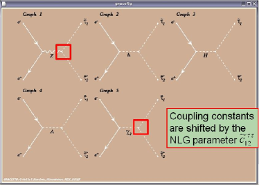
Figure 2: Feynman diagrams of the process $e^{-}+e^{+}\rightarrow\widetilde{\tau}^{-}_{1}+\widetilde{\tau}^{+}_{2}$ in tree-level order.

Figure 2 shows Feynman diagrams of the process $e^{-}+e^{+}\rightarrow\widetilde{\tau}^{-}_{1}+\widetilde{\tau}^{+}_{2}$ in tree-level order (drawn by gracefig), as an example. For this process, coupling constants of the vertices, $\widetilde{\tau}_{1}-\widetilde{\tau}_{2}-Z$ and $\widetilde{\tau}_{1}-\widetilde{\tau}_{2}-G^{0}(\chi_{3})$ are shifted by varying the NLG parameter $\tilde{c}_{12}^{\tau\tau}$, but the sum of the amplitudes is invariant. Here we set parameters as $M_{\widetilde{\tau}_{1}}$ = 320 GeV, $M_{\widetilde{\tau}_{2}}$ = 370 GeV, and total energy as $\sqrt{s}$ = 1000 GeV. The numerical results of the amplitude of each graph and the cross section at one point in the phase space are given in Table 4 for (case1) $\tilde{c}_{12}^{\tau\tau}$=0 and (case2) $\tilde{c}_{12}^{\tau\tau}$=1000. The total values in two cases agree up to 31 digits, so the NLG invariance of this process is confirmed in tree-level order.

Graph Absolute value of the amplitude case1: 1 1.6624897226795816149294531250854308$\times 10^{-3}$ 2 8.1590691554170053568905511607157850$\times 10^{-15}$ 3 1.9404461824036032871287809608655740$\times 10^{-10}$ 4 2.0390333192991456823825251175977558$\times 10^{-9}$ 5 5.6886720681154757343568160836757535$\times 10^{-14}$ total 1.6624919797058214816061810564292905$\times 10^{-3}$ case2: 1 1.6625481763453484261164965199981440$\times 10^{-3}$ 2 8.1590691554170053568905511607157850$\times 10^{-15}$ 3 1.9404461824036032871287809608655740$\times 10^{-10}$ 4 2.0390333192991456823825251175977558$\times 10^{-9}$ 5 5.8453722653531868198152256247220933$\times 10^{-8}$ total 1.6624919797058214816061810564293247$\times 10^{-3}$

Table 4: Tests for the NLG invariance

5 Summary

We have developed the program package GRACE/SUSY-loop for the EW corrections and QCD corrections of the MSSM amplitudes in one-loop order. Then we have calculated the radiative corrections to production processes and decay processes of SUSY particles in the framework of the MSSM using GRACE/SUSY-loop. We have also developed a version of GRACE/SUSY-loop for the extended NLG formalism by including bilinear forms of sfermions with new NLG parameters, and have carried out tests for it in tree-level order.

References

• [1] J. Fujimoto, T. Ishikawa, Y. Kurihara, M. Jimbo, T. Kon and M. Kuroda, Phys. Rev. D75 113002 (2007).
• [2] J. Fujimoto, T. Ishikawa, M. Jimbo, T. Kon, Y. Kurihara, M. Kuroda and M. Tomita, Automatic calculation of SUSY particle production and decay with GRACE/SUSY-loop, Talk presented at TOOLS 2008, http://indico.cern.ch/contributionDisplay.py?sessionId=19&contribId=42&confId=35476  (2008).
• [3] K. Iizuka, T. Ishikawa, Y. Kurihara, M. Kuroda, T. Kon, M. Jimbo and J. Fujimoto, 1 loop correction to sfermion decays with GRACE/SUSY-loop, Meeting abstracts of the Physical Society of Japan 63/2-1 22 (2008).
• [4] K. Iizuka, T. Kon, K. Kato, T. Ishikawa, Y. Kurihara, M. Jimbo and M. Kuroda, PoS RADCOR2009 068, [arXiv:hep-ph/1001.2800] (2010).
• [5] T. Kon, K. Iizuka, K. Kato, T. Ishikawa, Y. Kurihara, M. Jimbo and M. Kuroda, Light stop decay $\widetilde{t}_{1}\to bW^{+}\widetilde{\chi}^{0}_{1}$ in one-loop order in the MSSM using GRACE/SUSY-loop, (in preparation).
• [6] K. Fujikawa, Phys. Rev D7 393 (1973).
• [7] M.B. Gavela, G. Girardi, C. Malleville and P. Sorba, Nucl. Phys. B193 257 (1981).
• [8] H.E. Haber and D. Wyler, SCIPP-88/19 (1988).
• [9] M. Capdequi-Peyranère, H.E. Haber, P. Irulegui, PM-90-06, SCIPP-90-03, in Rigorous Methods in Particle Physics, Springer Tract. Phys. 119 (1990).
• [10] F. Boudjema and A. Chopin, Z. Phys. C73 85 (1996).
• [11] G. Bélanger, F. Boudjema, J. Fujimoto, T. Ishikawa, T. Kaneko, K. Kato, Y. Shimizu, Phys. Rept. 430 117 (2006).
• [12] J. Fujimoto, T. Ishikawa, M. Jimbo, T. Kaneko, T. Kon, Y. Kurihara, M. Kuroda and Y. Shimizu, Nucl. Phys. Proc. Suppl. 157 157 (2006).
• [13] F. Yuasa, J. Fujimoto, T. Ishikawa, M. Jimbo, T. Kaneko, K. Kato, S. Kawabata, T. Kon, Y. Kurihara, M. Kuroda, N. Nakazawa, Y. Shimizu and H. Tanaka, Prog. Theor. Phys. Suppl. 138 18 (2000);
http://minami-home.kek.jp/ .
• [14] N. Baro and F. Boudjema, Phys. Rev. D80 076010 (2009).
• [15] T. Hahn, Nucl. Phys. Proc. Suppl. 89 231 (2000); Comput. Phys. Commun. 140 418 (2001).
• [16] P.H. Chankowski, S. Pokorski and J. Rosiek, Nucl. Phys. B423 437 (1994).
• [17] A. Yamada, Phys. Lett. B263, 233 (1991); Z. Phys. C61 247 (1994).
• [18] A. Dabelstein, Z. Phys. C67 495 (1995).
• [19] W. Hollik, E. Kraus, M. Roth, C. Rupp, K. Sibold and D. Stöckinger, Nucl. Phys. B639 3 (2002).
• [20] T. Fritzsche and W. Hollik, Eur. Phys. J C24 619 (2002).
• [21] W. Siegel, Phys. Lett. B84 193 (1979).
• [22] D.M. Capper, D.R.T. Jones, P. van Nieuwenhuizen, Nucl. Phys. B167 479 (1980).
• [23] T. Fritzsche and W. Hollik, Nucl. Phys. Proc. Suppl. 135 102 (2004).
• [24] W. Öller, H. Eberl and W. Majerotto, Phys. Rev. D71 115002 (2005).
• [25] W. Killian, J. Reuter and T. Robens, Eur. Phys. J. C48 389 (2006); AIP Conf. Proc. 903 177 (2007).
• [26] M. Drees, W. Hollik and Q. Xu, JHEP 0702 032 (2007).
• [27] W. Beenakker, R. Hopker and P. M. Zerwas, Phys. Lett. B378 159 (1996).
• [28] W. Beenakker, R. Hopker, T. Plehn and P. M. Zerwas, Z. Phys. C75 349 (1997).
• [29] J. Guasch, J. Solà and W. Hollik, Phys. Lett. B437 88 (1998);
J. Guasch, W. Hollik and J. Solà, JHEP 10 040 (2002); LC-TH-2003-033, [arXiv:hep-ph/0307011] (2003).
• [30] J. A. Aguilar-Saavedra, et al., Eur. Phys. J. C46 43 (2006).