Transverse electron scattering response function of ³He with $\Delta$-isobar degrees of freedom

Abstract

A calculation of the ³He transverse $(e,e^{\prime})$ inclusive response function, $R_{T}$, which includes $\Delta$ degrees of freedom is performed using the Lorentz integral transform method. The resulting coupled equations are treated in impulse approximation, where the $NNN$ and $NN\Delta$ channels are solved separately. As NN and NNN potentials we use the Argonne V18 and UrbanaIX models respectively. Electromagnetic currents include the $\Delta$-isobar currents, one-body N-currents with relativistic corrections and two-body currents consistent with the Argonne V18 potential. $R_{T}$ is calculated for the breakup threshold region at momentum transfers near 900 MeV/c. Our results are similar to those of Deltuva et al. in that large $\Delta$-isobar current contributions are found. However we find that these are largely canceled by the relativistic contribution from the one-body N-currents. Finally a comparison is made between theoretical results and experimental data.

I Introduction

It is well known RhoWil that subnuclear degrees of freedom play an important role in nuclear dynamics. In conventional low-energy nuclear physics the relevant subnuclear degrees of freedom are considered to be mesons and nucleon isobars. Electron scattering affords an excellent tool for studying these degrees of freedom which are manifested in the transverse response through meson exchange (MEC) and isobar (IC) currents. The consideration of such subnuclear currents has a long history in the physics of few-nucleon systems. For two-body systems a review can be found in ALT05 . One important issue in the MEC is their consistency with the nucleon-nucleon ($NN$) potential being used. Such consistent MEC’s have not only been taken into account in deuteron electrodisintegration, but also in the electrodisintegration of three-body systems ViK00 ; Golak05 ; Deltuva1 ; DEKLOTY08 ; LEOT10 . On the other hand IC have not received the attention in three-body systems which they have in the two-nucleon sector. Nevertheless there exists a rather complete calculation by Deltuva1 ; Yuan02 ; Deltuva04 where $N$ and $\Delta$ degrees of freedom have been treated on an equivalent level via a coupled channel calculation with $NNN$ and $NN\Delta$ channels. Also $\Delta$-effects have been studied ViK00 in ³He electrodisintegration below the three-body breakup threshold using the transition-correlation-operator method ScW92 .

The present work incorporates the dynamics of the $\Delta$-resonance into the many-body wavefunction by means of the impulse approximation (IA) WeA78 . This method, as in the transition-correlation-operator and coupled channel methods, avoids the static approximation by fully including the kinetic energy in the $\Delta$-propagator. For electromagnetic deuteron breakup it has been shown that the $\Delta$-effects resulting from an IA calculation are rather similar to those resulting from a coupled channel calculation if the energy is sufficiently below the resonance position of the $\Delta$ LA87 .

A calculation of $R_{T}$ in our case requires an integration over continuum states of the coupled NNN + NN$\Delta$ system. As has been demonstrated previously ELO94 ; ELOB07 the Lorentz integral transform (LIT) method is well suited for calculating inclusive quantities such as response functions. Examples of its use in calculating electron scattering response functions of three- and four-body nuclei employing realistic nuclear forces (two- and three-body forces) include (i) nonrelativistic calculations of $R_{L}$ for three-nucleon systems ELOT04 , for ⁴He BBLO09 and inclusion of relativistic effects in ³H and ³He ELOT05 and (ii) calculations of $R_{T}$ with relativistic and consistent MEC contributions for three-body nuclei DEKLOTY08 ; LEOT10 ; ELOT10 . There is an LIT calculation BABLO07 of $R_{T}$ for ⁴He but with semi-realistic $NN$ forces. The method has not previously been applied to the coupled NNN+NN$\Delta$ system so that this paper is the first in that regard.

The paper is organized as follows. In section II we describe the general formalism including the incorporation of $\Delta$ degrees of freedom in the LIT formalism. Section III specifies the input to the dynamical equations developed in section II. This includes subsection A detailing the potentials used in the NNN and NN$\Delta$ sectors, subsection B describing the electromagnetic current operators used and subsection C outlining calculational details. Finally our results are discussed in section IV. There we compare our results for $R_{T}$ to those from another calculation and to experimental data.

II Formalism

In the one photon exchange approximation the cross section for the process of inclusive electron scattering on a nucleus is given by

$${d^{2}\sigma\over d\Omega\,d\omega}\ =\ \sigma_{Mott}\ \bigg{[}\ {Q^{4}\over q^{4}}\,R_{L}(q,\omega)\ +\ \left(\ {Q^{2}\over 2q^{2}}+\tan^{2}{\theta\over 2}\ \right)\,R_{T}(q,\omega)\bigg{]}\,,$$ (1)

where $R_{L}$ and $R_{T}$ are the longitudinal and transverse response functions respectively, $\omega$ is the electron energy loss, $q$ is the magnitude of the electron momentum transfer, $\theta$ is the electron scattering angle, and $Q^{2}=q^{2}-\omega^{2}$.

In the present work we study the transverse response function,

$$R_{T}(q,\omega)={\overline{\sum}}_{M_{i}}\sum\!\!\!\!\!\!\!\int\,df({\bf j}_{t}^{\dagger})_{if}\cdot({\bf j}_{t})_{fi}\delta(E_{\bar{f}}-E_{i}-\omega)$$ (2)

with $\Delta$ degrees of freedom within a non-relativistic approach. The low $\omega$ region is considered. In (2) the subscripts $i$ and $f$ label, respectively, an initial state and final states, and the matrix elements are taken between internal states, center-of-mass motion being excluded.

As mentioned in the introduction we employ the IA in order to take into account the $\Delta$-resonance. This approximation is used for both the ³He ground state and the final state. Below we outline the various theoretical aspects required to include $\Delta$ degrees of freedom in a calculation of $R_{T}$ via the LIT method.

We consider the three-nucleon system with $N(939)$ and $\Delta(1232)$ degrees of freedom, which leads to the following Hamiltonian

$$H=T+\delta m+V=\sum_{i=1}^{3}(T_{i}+\delta m_{i})+\sum^{3}_{i<j}V_{ij}\,,$$ (3)

where $T_{i}$ is the kinetic energy of particle $i$ with mass $m_{i}$, $\delta m_{i}=m_{i}-m_{N}$ is its mass difference with nucleon $N(939)$, and $V_{ij}=V_{ji}$ is the potential between particles $i$ and $j$. By omitting the contribution from more than one $\Delta$-isobar excitation, we construct the three-particle bound state from an $NNN$ part and a $NN\Delta$ part i.e.,

$$|\Psi_{0}\rangle=|\Psi^{N}_{0}\rangle+|\Psi^{\Delta}_{0}\rangle\,.$$ (4)

The wave function is determined by the Schrödinger equation

$$(T_{N}+\bar{V}^{NN}-E)|\Psi^{N}_{0}\rangle = -V^{NN,N\Delta}\ |\Psi^{\Delta}_{0}\rangle\,,$$ (5)

$$(H_{\Delta}-E)|\Psi^{\Delta}_{0}\rangle=(\delta m+T_{\Delta}+V^{N\Delta}-E)|\Psi^{\Delta}_{0}\rangle = -V^{N\Delta,NN}|\Psi^{N}_{0}\rangle\,,$$ (6)

where $V^{N^{\prime}_{1}N^{\prime}_{2},N_{1}N_{2}}=\sum^{3}_{i<j}V_{ij}(N_{1}N_{2}\rightarrow{N^{\prime}_{1}N^{\prime}_{2}}),\quad\bar{V}^{NN}=\bar{V}^{NN,NN},\quad V^{N\Delta}=V^{N\Delta,N\Delta}$, and $\sum^{3}_{i=1}T_{i}$ is denoted by $T_{N}$ and $T_{\Delta}$ for the $NNN$ and $NN\Delta$ channels, respectively. One should note that $\bar{V}^{NN}$ is different from the usual sum of realistic $NN$ potentials, $V^{NN}$, because the latter already contain implicit effects due to the $\Delta$ (e.g., in meson theoretical $NN$ potentials realized via part of the $\sigma$ meson exchange).

Here we do not search for a direct solution of the coupled channel problem represented by Eqs. (5,6). Instead we use the IA where one computes $\Psi^{N}_{0}$ and $\Psi^{\Delta}_{0}$ separately. More specifically one first determines the $NNN$ part by solving

$$(H_{N}-E)|\Psi^{N}_{0}\rangle=0$$ (7)

with

$$H_{N}=T_{N}+V^{NN}+V^{NNN}\,,$$ (8)

where $V^{NNN}=\sum^{3}_{i<j<k}V_{ijk}$ is a three-nucleon force. In the IA one then uses the solution $|\Psi^{N}_{0}\rangle$ in order to calculate $|\Psi^{\Delta}_{0}\rangle$ through (6).

Treatment of the continuum in the LIT technique requires the calculation of a localized Lorentz state $|\tilde{\Psi}\rangle$. This Lorentz state $|\tilde{\Psi}\rangle$ also has $NNN$ and $NN\Delta$ parts written as

$$|\tilde{\Psi}\rangle=|\tilde{\Psi}^{N}\rangle+|\tilde{\Psi}^{\Delta}\rangle\,.$$ (9)

These fulfill the coupled equations

$$(T_{N}+\bar{V}^{NN}-E_{0}-\sigma)|\tilde{\Psi}^{N}\rangle = -V^{NN,N\Delta}\ |\tilde{\Psi}^{\Delta}\rangle+{O}_{NN}|\Psi^{N}_{0}\rangle+{O}_{N\Delta}|\Psi^{\Delta}_{0}\rangle\,,$$ (10)

$$(\delta m+T_{\Delta}+V^{N\Delta}-E_{0}-\sigma)|\tilde{\Psi}^{\Delta}\rangle = -V^{N\Delta,NN}|\tilde{\Psi}^{N}\rangle+{O}_{\Delta N}|\Psi^{N}_{0}\rangle+{O}_{\Delta\Delta}|\Psi^{\Delta}_{0}\rangle\,,$$ (11)

where $E_{0}$ is the three-body ground-state energy, the complex $\sigma=\sigma_{R}+i\sigma_{I}$ is the argument of the LIT in the transformed space, and the ${O}_{N_{1}N_{2}}$ denote the various diagonal ($N_{1}=N_{2})$) and transition ($N_{1}\neq N_{2})$ electromagnetic current operators. One first solves for the $NNN$ part using $H_{N}$ of Eq. (8):

$$(H_{N}-E_{0}-\sigma)|\tilde{\Psi}^{N}\rangle = -V^{NN,N\Delta}(H_{\Delta}-E_{0}-\sigma)^{-1}\left({O}_{\Delta N}|\Psi^{N}_{0}\rangle+{O}_{\Delta\Delta}|\Psi^{\Delta}_{0}\rangle\right)$$ (12)

$$+{O}_{NN}|\Psi^{N}_{0}\rangle+{O}_{N\Delta}|\Psi^{\Delta}_{0}\rangle\,.$$

The above equation is derived by solving (11) formally for $|\tilde{\Psi}^{\Delta}\rangle$, inserting the solution in (10), and dropping the term $V^{NN,N\Delta}(H_{\Delta}-E_{0}-\sigma)^{-1}V^{N\Delta,NN}$, since, as mentioned, $\Delta$-effects to the nuclear interaction are already contained in the realistic $H_{N}$. With $|\tilde{\Psi}^{N}\rangle$ thus obtained one then calculates $|\tilde{\Psi}^{\Delta}\rangle$ in a second step through (11). Given the solutions $|\tilde{\Psi}^{N}\rangle$ and $|\tilde{\Psi}^{\Delta}\rangle$ the LIT is obtained from the norm of the Lorentz state as

$$\langle\tilde{\Psi}|\tilde{\Psi}\rangle\ =\ \langle\tilde{\Psi}^{N}|\tilde{\Psi}^{N}\rangle+\langle\tilde{\Psi}^{\Delta}|\tilde{\Psi}^{\Delta}\rangle.$$ (13)

These two terms correspond to different contributions. It can be shown that the piece $\langle\tilde{\Psi}^{N}|\tilde{\Psi}^{N}\rangle$ describes contributions due to final states with nucleons only. In this case the $\Delta$ degrees of freedom only contribute as virtual intermediate states. On the contrary the term $\langle\tilde{\Psi}^{\Delta}|\tilde{\Psi}^{\Delta}\rangle$ describes contributions from final states containing a real $\Delta$. The contribution to $R_{T}$ from this term vanishes below the threshold for $\Delta$ production. Since the present study is for energies below that threshold this term will not contribute here to $R_{T}$. Such a real $\Delta$ has to decay into a nucleon and a pion eventually, thus the contribution $\langle\tilde{\Psi}^{\Delta}|\tilde{\Psi}^{\Delta}\rangle$ corresponds to resonant pion production.

III Input to Dynamical Equations

III.1 Potentials

In the pure nucleonic sector we use the Argonne V18 (AV18) NN potential AV18 and the Urbana IX (UIX) NNN potential UIX while for the pure NN$\Delta$ sector we take $V^{N\Delta}$=0 as in the IA calculation of LA87 . The NNN and NN$\Delta$ sectors are coupled via the $V^{NN,N\Delta}$ and $V^{N\Delta,NN}$ potentials. We use the same form for this potential as described in LA87 except that here we use the short range cutoff given in the AV18 AV18 potential. In detail we take $V(NN\to N\Delta)$ between particles 1 and 2 to have the form

$$V_{12}=a_{NN^{\prime}\pi}{\boldsymbol{\tau}}_{1}\!\cdot\!{\boldsymbol{\tau}}_{2}\left\{\left[V_{0}(m_{\pi})+\frac{2a_{NN^{\prime}\rho}}{a_{NN^{\prime}\pi}}V_{0}(m_{\rho})\right]{\boldsymbol{\sigma}}_{1}\!\cdot\!{\boldsymbol{\sigma}}_{2}\right.$$

$$\left.+\left[V_{2}(m_{\pi})-\frac{a_{NN^{\prime}\rho}}{a_{NN^{\prime}\pi}}V_{2}(m_{\rho})\right]S_{12}\right\}$$ (14)

with

$$V_{0}(m)=(mr)^{-1}e^{-mr}(1-e^{-cr^{2}}),$$ (15)

$$V_{2}(m)=\left[1+\frac{3}{mr}+\frac{3}{(mr)^{2}}\right]\frac{e^{-mr}}{mr}(1-e^{-cr^{2}})^{2},$$ (16)

where ${\boldsymbol{\sigma}}_{i}$ $({\boldsymbol{\tau}}_{i})$ are regarded as transition operators for spin (isospin) of particle $i$, the coupling constants $a_{NN^{\prime}\pi}$ and $a_{NN^{\prime}\rho}$ are taken from LA87 , $c=2.1\;\mbox{fm}^{-2}$ is the same value as in the AV18 potential, and $r=|{\bf r}_{1}-{\bf r}_{2}|$ is proportional to the Jacobi vector ${\boldsymbol{\xi}}_{1}$ (see Eq. (22)).

III.2 Electromagnetic Currents

In Eqs. (10) and (11) the driving terms are the transverse electromagnetic currents acting on the ground state. The term $O_{NN}$ represents the purely nucleonic one- and two-body currents. For these the same one-body and two-body currents as employed in ELOT10 are used. There the one-body currents included relativistic corrections to order $M^{-3}$ and the two-body currents were consistent $\pi$- and $\rho$-MEC currents constructed using the method of Arenhövel and Schwamb AS . The other terms $O_{N\Delta}$, $O_{\Delta N}$, and $O_{\Delta\Delta}$ are transition and diagonal one-body $\Delta$-isobar currents. The currents involving the $\Delta$-resonance are given in Fig. 1. For one-body $\Delta$-isobar currents we use the forms

$${\bf j}_{\Delta N}=\ \sum_{k=1}^{3}e^{i{\bf q}\cdot{\bf r}_{k}^{\prime}}\ \frac{i({\sigma_{k}}^{\Delta N}\times{\bf q})}{2m_{\Delta}}\ G^{\Delta N}_{M1}\tau_{zk}^{\Delta N},$$ (17)

and

$${\bf j}_{\Delta\Delta}=\ \sum_{k=1}^{3}e^{i{\bf q}\cdot{\bf r}_{k}^{\prime}}\ \left[\frac{2{\bf p}_{k}^{\prime}+\kappa{\bf q}}{2m_{\Delta}}\ G^{\Delta}_{E0}+\ \frac{i({\sigma_{k}}^{\Delta}\times{\bf q})}{2m_{\Delta}}\ \ G^{\Delta}_{M1}\right]\frac{1+\tau_{zk}^{\Delta}}{2},$$ (18)

where ${\bf r}_{k}^{\prime}={\bf r}_{k}-{\bf R}_{cm}$, and ${\bf p}_{k}^{\prime}={\bf p}_{k}-{\bf P}_{cm}A_{k}/A$ are the relative coordinate and momentum operator of the k-th particle, while ${\bf R}_{cm}$ and ${\bf P}_{cm}$ are the center-of-mass coordinate and initial total momentum variables of the system. With the assumption that ${\bf P}_{cm}$ is directed along $\bf q$ the term $\kappa$ in (18) has the value $\kappa=1+2P_{cm}A_{k}/(Aq)$. However since here we are dealing with transverse currents this term does not contribute. The formfactors for the above currents are the same as in Deltuva1 ; Deltuva04 and take the form

$$G^{\Delta N}_{M1}(Q^{2})={\frac{m_{\Delta}}{m_{N}}}\frac{4.59}{(1+Q^{2}/{\Lambda}^{2}_{\Delta N1})^{2}(1+Q^{2}/{\Lambda}^{2}_{\Delta N2})^{1/2}},$$

$$G^{\Delta}_{E0}(Q^{2})=G^{p}_{E}(Q_{2}),$$ (19)

$$G^{\Delta}_{M1}(Q^{2})={\frac{m_{\Delta}}{3m_{N}}}\frac{(4.35/2.0)}{(1+Q^{2}/{\Lambda}^{2}_{\Delta N1})^{2}}$$

with ${\Lambda}_{\Delta N1}=840$ MeV and ${\Lambda}_{\Delta N2}=1200$ MeV . As in our previous $NNN$ calculations DEKLOTY08 ; LEOT10 ; ELOT10 we use the approximations

$$G_{M1}^{\Delta N}(Q^{2})\approx{\bar{\mu}}^{\Delta N}_{p}(Q_{av}^{2})G_{E}^{p}(Q^{2}),\qquad\qquad{\bar{\mu}}^{\Delta N}_{p}(Q_{av}^{2})=\frac{G^{\Delta N}_{M1}(Q_{av}^{2})}{G_{E}^{p}(Q_{av}^{2})},$$

$$G_{M1}^{\Delta}(Q^{2})\approx{\bar{\mu}}^{\Delta}_{p}(Q_{av}^{2})G_{E}^{p}(Q^{2}),\qquad\qquad{\bar{\mu}}^{\Delta}_{p}(Q_{av}^{2})=\frac{G_{M1}^{\Delta}(Q_{av}^{2})}{G_{E}^{p}(Q_{av}^{2})},$$

.

Figure 1: Operators involving the $\Delta$-resonance in the $NNN$ (a) and $NN\Delta$ (b) channels

III.3 Calculational Details

In order to solve Eqs. (7), (11) and (12) for the ground state and Lorentz vectors we expand the bound and Lorentz states on a complete antisymmetric basis. The reason for antisymmetrizing NN$\Delta$ states is that they couple to purely antisymmetric nucleonic states through symmetric operators. Thus the excitation of an antisymmetric NNN state to a $NN\Delta$ state occurs via an operator symmetric with respect to nucleons. Such an operator is a sum of operators which replace a nucleon with a $\Delta$ which therefore leads to an antisymmetric $NN\Delta$ state. For the $NNN$ part we take the same correlated hyperspherical basis as in our previous three-body calculations without considering $\Delta$ degrees of freedom (see, e.g., ELOB07 ). For the part with one $\Delta$-excitation we use the following hyperspherical basis

$$|\varphi_{k}\rangle=\frac{1+P}{\sqrt{3}}\frac{1-(12)}{\sqrt{2(1+B^{2})}}\left|\left(h_{NK(Ll)\mathcal{L}}\otimes\left(\left(s_{1}s_{2}\right)Ss_{3}\right)\mathcal{S}\right)_{\mathcal{JM_{J}}},\left(\left(t_{1}t_{2}\right)Tt_{3}\right)\mathcal{TM_{T}}\right\rangle\,,$$ (20)

where $N$ is the order of the hyperradial function, $K$ is the hyperspherical angular momentum, $L$ and $l$ are the orbital angular momentum of the pair and of the spectator, respectively, coupled to the total orbital angular momentum $\mathcal{L}$. Individual spin (isospin) quantum numbers of the three particles are denoted by $s_{i}$ $(t_{i}),$ $i=1,2,3$ while the pair spin (isospin) is denoted by $S$ ($T$), the total spin (isospin) by $\mathcal{S}$ ($\mathcal{T}$) and $\mathcal{M_{T}}$ stands for the projection of the total isospin. Quantum numbers ${\mathcal{J}}$ and ${\mathcal{M}_{J}}$ denote the total angular momentum and its projection and $(...\otimes...)_{\mathcal{J}M_{J}}$ denotes $\mathcal{(LS)J}$ coupling. The index $k$ denotes collectively $\{N,K,L,l,\mathcal{L},S,\mathcal{S},{\mathcal{J,M_{J}}},T,\mathcal{T,M_{T}}\}$ and $B$. We define the quantity $B$ to be 0 if the pair of the three particle system contains one $\Delta$ and therefore $(s_{1},s_{2},s_{3})=(t_{1},t_{2},t_{3})=(1/2,3/2,1/2)$, and to be 1 if the pair contains no $\Delta$ and therefore $(s_{1},s_{2},s_{3})=(t_{1},t_{2},t_{3})=(1/2,1/2,3/2)$. Note that if particles 1 and 2 are nucleons we always assume that L+S+T=odd so that the NN pair is already antisymmetric. The spatial basis functions in coordinate representation are products of hyperradial functions and hyperspherical harmonics

$$\langle{\boldsymbol{\xi}}_{1}{\boldsymbol{\xi}}_{2}|h_{NK(Ll)\mathcal{LM_{L}}}\rangle=R_{N}(\rho)Y^{Ll}_{K\mathcal{LM_{L}}}(x,x_{1},\varphi_{1},x_{2},\varphi_{2}),$$ (21)

The coordinates $\rho$ and $x$ are defined in terms of the Jacobi vectors

$${\boldsymbol{\xi}}_{1} = \sqrt{\frac{A_{1}A_{2}}{A_{1}+A_{2}}}\left({\bf r}_{2}-{\bf r}_{1}\right),\;\;{\boldsymbol{\xi}}_{2}=\sqrt{\frac{(A_{1}+A_{2})A_{3}}{A_{1}+A_{2}+A_{3}}}\left({\bf r}_{3}-\frac{A_{1}{\bf r}_{1}+A_{2}{\bf r}_{2}}{A_{1}+A_{2}}\right)$$ (22)

as $\rho=(\xi_{1}^{2}+\xi_{2}^{2})^{1/2}$, $x=(\xi_{2}^{2}-\xi_{1}^{2})/\rho$. The coordinates $x_{i}\equiv\cos\theta_{i}$ and $\varphi_{i}$ are spherical coordinates of the unit vectors in the directions of ${\boldsymbol{\xi}}_{1}$ and ${\boldsymbol{\xi}}_{2}$. We use the notation $A_{i}\equiv{m_{i}}/{m_{N}}$. Note that particle permutations entering the antisymmetrization operator interchange not only particle position vectors ${\bf r}_{i}$ but also their mass numbers $A_{i}$. One has $\rho^{2}=\xi_{1}^{2}+\xi_{2}^{2}=A_{1}r_{1}^{2}+A_{2}r_{2}^{2}+A_{3}r_{3}^{2}-AR^{2}$, where ${\bf R}$ is the center-of-mass position. Thus $\rho$ remains invariant under particle permutations.

The operator $\left(1-(12)\right)/\left[2(1+B^{2})\right]^{1/2}$ makes the (12)-pair explicitly antisymmetric. Note that it gives unity if the pair contains no $\Delta$ but rather is an antisymmetric NN pair. Finally the operator ${(1+P)}/{\sqrt{3}}$, where $P\equiv(123)+(132)$, makes the three particle states with antisymmetric (12) pair totally antisymmetric. It turns out to be convenient to keep both $B=0$ and $B=1$ in (20) (thereby resulting in an overcomplete basis) and to finally select out numerically the linearly independent states. This enables one to select out those states which give negligible contributions to the results. Application of the operator ${(1+P)}/{\sqrt{3}}$ in (20) results in the more practical form

$$|\varphi_{k}\rangle=\sum_{B^{\prime}S^{\prime}T^{\prime}}\frac{1-(12)}{\sqrt{2(1+B^{{}^{\prime}2})}}\left|\left(F_{j\mathcal{L}}\otimes\left(\left(s_{1}^{\prime}s_{2}^{\prime}\right)S^{\prime}s_{3}^{\prime}\right)\mathcal{S}\right)_{\mathcal{JM_{J}}},\left(\left(t_{1}^{\prime}t_{2}^{\prime}\right)T^{\prime}t_{3}^{\prime}\right)\mathcal{TM_{T}}\right\rangle,$$ (23)

where $j$ denotes collectively $\{B^{\prime}S^{\prime}T^{\prime},BS\mathcal{S}T\mathcal{T}NK(Ll)\}$ and

$$\left|F_{j\mathcal{L}\mathcal{M_{L}}}\right\rangle =\frac{1}{\sqrt{3}}\Big{(}\delta_{B^{\prime},B}\delta_{S^{\prime},S}\delta_{T^{\prime},T}\left|h_{NK(Ll)\mathcal{L}\mathcal{M_{L}}}\right\rangle$$ (24)

$$+g^{c}_{B^{\prime}S^{\prime}T^{\prime},BS\mathcal{S}T\mathcal{T}}\left|h^{c}_{NK(Ll)\mathcal{L}\mathcal{M_{L}}}\right\rangle+g^{d}_{B^{\prime}S^{\prime}T^{\prime},BS\mathcal{S}T\mathcal{T}}\left|h^{d}_{NK(Ll)\mathcal{L}\mathcal{M_{L}}}\right\rangle\Big{)}$$

with $(Ll)\mathcal{L}$ coupling for the total orbital angular momentum $\mathcal{L}$ and its projection $\mathcal{M_{L}}$. As mentioned above components with $B^{\prime}$=1 in Eq. (23) represent configurations NN$\Delta$ in which particles 1 and 2 are nucleons. Those components with $B^{\prime}$=0 represent N$\Delta$N configurations in which particle 1 is a nucleon and particle 2 is a $\Delta$. More details of the spin-isospin factors $g^{c}$ and $g^{d}$, and the spatial functions $h^{c}$ and $h^{d}$ are given in Appendix A. Techniques employed in calculating the kinetic energy and the $NN\to N\Delta$ or $N\Delta\to NN$ potential are given in Appendices B and C respectively.

As in DEKLOTY08 all currents are expressed in terms of multipole expansions. Explicit expressions for the multipoles of the one-body current (containing relativistic corrections) are given in ELOT10 . The multipoles for the $\pi$- and $\rho$-MEC are found in DEKLOTY08 with modifications due to the implementation of consistent MECs for the AV18 potential listed in LEOT10 . Finally the multipoles required here for the one-body currents relating to the $\Delta$ are listed in Appendix D. With these multipoles one can then decompose the LIT of the response function according to its multipole content as

$$\tilde{R_{T}}(\sigma)=\frac{4\pi}{2{\mathcal{J}}_{0}+1}\sum_{\lambda={\rm el,mag}}\sum_{{\mathcal{J}}j}(2{\mathcal{J}}+1)(\tilde{R_{T}})_{\mathcal{J}}^{j\lambda}\,,$$ (25)

where

$$(\tilde{R_{T}})_{\mathcal{J}}^{j\lambda}=\langle\tilde{\Psi}^{j\lambda}_{\mathcal{J}M}|\tilde{\Psi}^{j\lambda}_{\mathcal{J}M}\rangle=\langle\tilde{\Psi}^{Nj\lambda}_{\mathcal{J}M}|\tilde{\Psi}^{Nj\lambda}_{\mathcal{J}M}\rangle+\langle\tilde{\Psi}^{\Delta j\lambda}_{\mathcal{J}M}|\tilde{\Psi}^{\Delta j\lambda}_{\mathcal{J}M}\rangle.$$ (26)

Here ${\mathcal{J}}_{0}$ is the initial state total angular momentum, ${\mathcal{J}}$ and ${\mathcal{M}}$ are the final state total angular momentum and its projection. The $|\tilde{\Psi}^{j\lambda}_{\mathcal{J}}\rangle$ are the solutions of (11,12) where the following replacement is made on the rhs of these equations

$$O|\Psi_{0}\rangle\rightarrow|q_{{\mathcal{J}}{\mathcal{M}}}^{j\lambda}\rangle=[T_{j}^{\lambda}\otimes|\Psi_{0}({\mathcal{J}}_{0})\rangle]_{{\mathcal{J}}{\mathcal{M}}}.$$ (27)

In Eq. (26) ${\mathcal{M}}$ is arbitrary. In Eq. (27) above $\Psi_{0}$ is either $\Psi^{N}_{0}$ or $\Psi^{\Delta}_{0}$, while $O$ represents the various electromagnetic current operators on the rhs of (10,11). By projecting the rhs of (27) on the basis states (23) one obtains

$$\left\langle\left(F_{j^{\prime}\mathcal{L^{\prime}}}\otimes\left(\left(s_{1}^{\prime}s_{2}^{\prime}\right)S^{\prime}s_{3}^{\prime}\right)\mathcal{S^{\prime}}\right)_{\mathcal{J^{\prime}M^{\prime}}}\right|q_{{\mathcal{J}}{\mathcal{M}}}^{j\lambda}\rangle=\delta_{\mathcal{J^{\prime},J}}\delta_{\mathcal{M^{\prime},M}}\frac{\left\langle\left(F_{j^{\prime}\mathcal{L^{\prime}}}\otimes\left(\left(s_{1}^{\prime}s_{2}^{\prime}\right)S^{\prime}s_{3}^{\prime}\right)\mathcal{S^{\prime}}\right)_{\mathcal{J^{\prime}}}\right\|T_{j}^{\lambda}\|\Psi_{0}({\mathcal{J}}_{0})\rangle}{\hat{\mathcal{J}^{\prime}}}.$$ (28)

We use the Lanczos method to calculate the response function, as described in MBLO03 . The response function is thus calculated by using

$$\langle\tilde{\Psi}^{Nj\lambda}_{\mathcal{JM}}|\tilde{\Psi}^{Nj\lambda}_{\mathcal{JM}}\rangle=-\frac{1}{\sigma_{I}}Im\langle Q^{j\lambda}_{\mathcal{JM}}|\frac{1}{E_{0}+\sigma-H_{N}}|Q^{j\lambda}_{\mathcal{JM}}\rangle$$

$$=-\sum_{m,n}\frac{1}{\sigma_{I}}Im\langle Q^{j\lambda}_{\mathcal{JM}}|\phi_{m}\rangle\langle\phi_{m}|\frac{1}{E_{0}+\sigma-H_{N}}|\phi_{n}\rangle\langle\phi_{n}|Q^{j\lambda}_{\mathcal{JM}}\rangle\,,$$ (29)

where $Q$ corresponds to the rhs of (12) and $|\phi_{n}\rangle$ is the set of orthogonal Lanczos vectors. As starting vector $|\phi_{0}\rangle$ we choose the rhs of (12) at one particular value of $\sigma$. The expression $\langle\phi_{m}|({E_{0}+\sigma-H_{N}})^{-1}|\phi_{n}\rangle$ can be calculated by using Eq. (71) of MBLO03 . A difference from previous LIT applications appears in the potential term on the rhs of the LIT equation, namely the $N\Delta$ transition potential $V^{NN,N\Delta}$ in (12). The contribution of this term to $\langle\phi_{n}|Q^{j\lambda}_{\mathcal{JM}}\rangle$ is given by

$$-\sum_{l^{\prime}k^{\prime}lkm}\langle\phi_{n}|\varphi_{l^{\prime}}\rangle N^{-1}_{l^{\prime}k^{\prime}}\langle\varphi_{k^{\prime}}|V^{NN,N\Delta}|\varphi_{l}\rangle N^{-1}_{lk}\langle\varphi_{k}|\phi_{m}\rangle\langle\phi_{m}|(H_{\Delta}-E_{0}-\sigma)^{-1}|q^{j\lambda}_{\mathcal{JM}}\rangle,$$ (30)

with

$$|q^{j\lambda}_{\mathcal{JM}}\rangle=[{\cal T}_{\Delta N,j}^{\lambda}\otimes|\Psi^{N}_{0}({\mathcal{J}}_{0})\rangle]_{{\mathcal{J}}{\mathcal{M}}}+[{\cal T}_{\Delta\Delta,j}^{\lambda}\otimes|\Psi^{\Delta}_{0}({\mathcal{J}}_{0})\rangle]_{{\mathcal{J}}{\mathcal{M}}},$$ (31)

and the norm matrix $N=\left(\left\langle\varphi_{k}|\varphi_{l}\right\rangle\right)$. Also the second term in Eq. (26), $\langle\tilde{\Psi}^{\Delta j\lambda}_{\mathcal{J}M}|\tilde{\Psi}^{\Delta j\lambda}_{\mathcal{J}M}\rangle$, can be calculated in a similar way with the Lanczos method.

Because in this paper we are working at low energies near the ³He breakup threshold only the lowest multipole transitions contribute. We found sufficient accuracy by restricting the maximum value of $\mathcal{J}$ to 5/2. The LIT is computed with $\sigma_{I}=5$ MeV. The LIT inversion BELO10 is made with our standard inversion method ELOB07 ; ALRS05 . As discussed in DEKLOTY08 we subtract from the LIT of the M1 transition the elastic contribution and invert the remaining inelastic piece separately from the other multipole contributions.

IV Results

In the present work we have used the LIT method to calculate $\Delta$-IC effects on the transverse electron scattering response function $R_{T}(q,\omega)$ for q$\approx$900 MeV/c and $\omega$ up to 20 MeV above the breakup threshold. This is the first application of the LIT method to include $\Delta$ degrees of freedom in the calculation of inclusive (e,e’) response functions. The importance of $\Delta$-effects at these kinematics has previously been shown by Deltuva1 . As $NN$ and $NNN$ interactions we used the AV18 and the UIX potentials respectively. Following the IA calculation of LA87 we do not consider a diagonal N$\Delta$ interaction, i.e. $V_{N\Delta}=0$. For the ³He ground state, our interaction model leads to a $\Delta$-probability of 1.14 % which compares to 1.44% obtained by Deltuva1 who used a CDBonn+$\Delta$ coupled channel potential model DeM03 . In addition to the $\Delta$-ICs ${\bf j}_{N\Delta}$, ${\bf j}_{\Delta N}$ and ${\bf j}_{\Delta\Delta}$ the purely nucleonic currents include the nonrelativistic one-body current with relativistic corrections up to order $M^{-3}$ ELOT10 and an MEC consistent with the AV18 potential LEOT10 . Concerning the relativistic corrections we leave out the $\omega$ dependent relativistic piece in the present work as its contribution is negligible in the threshold region we consider. For the neutron magnetic and the proton form factors we take the dipole fit while the neutron electric form factor is taken from GaK71 .

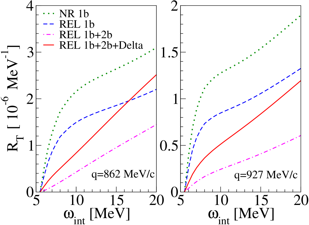
Figure 2: Theoretical results for $R_{T}$ of ³He as function of internal excitation energy $\omega_{\rm int}$ at $q$=862 and 927 MeV/c with various current operators: non-relativistic nucleon one-body (dotted), with additional relativistic corrections (dashed), plus additional MEC (dash-dotted), further addition of $\Delta$-IC (solid).

Fig. 2 displays our $R_{T}$ results for several calculational options. The dominant transition multipolarity contributing at these near threshold energies is M1. One sees that relativistic effects reduce the M1 transition strength considerably. If in addition MEC are also taken into account then the M1 contribution drops markedly leading to a rather different low-energy behavior of $R_{T}$. Inclusion of $\Delta$-IC restores some of this lost strength and demonstrates, as anticipated, that the $\Delta$ effect is quite large.

Now we turn to a comparison of our results with those of Deltuva1 . For the comparison one should keep in mind that there are differences between the two calculations. Thus in Deltuva1 , (i) relativistic currents have not been considered, (ii) the Coulomb force is neglected in the final state interaction, (iii) their nucleonic potential model, the CDBonn CDBonn , is different from ours and does not reproduce the ³He binding energy and (iv) the full coupled channel calculation, CDBonn+$\Delta$ DeM03 , is a more consistent treatment of $\Delta$ degrees of freedom than the IA, but leads to a slight underestimation of the ³He binding energy. There is another point which makes the comparison a bit more difficult. Namely, the $R_{T}$ of Deltuva1 is not calculated for a constant momentum transfer, in fact $q$ is slightly decreasing with growing energy. Therefore, in Fig. 3, we prefer to display the results for each $q$ in two panels. One sees that despite the various differences mentioned above the $\Delta$-effects in both calculations are very similar. However, one also notes that relativistic corrections lead to an opposite effect, which is of the same size at $q=862$ MeV/c, but somewhat weaker at $q=927$ MeV/c. By comparison of results for $R_{T}$ at about $q=500$ MeV/c from LEOT10 against those of Deltuva1 one finds again an at least partial cancellation of relativistic and $\Delta$ contributions close to the breakup threshold. The stronger increase of $R_{T}$ in the calculation of Deltuva1 at higher energies, seen in Fig. 3, partly originates from the non-constant momentum transfers used in Deltuva1 as mentioned above (see also discussion of Fig. 4).

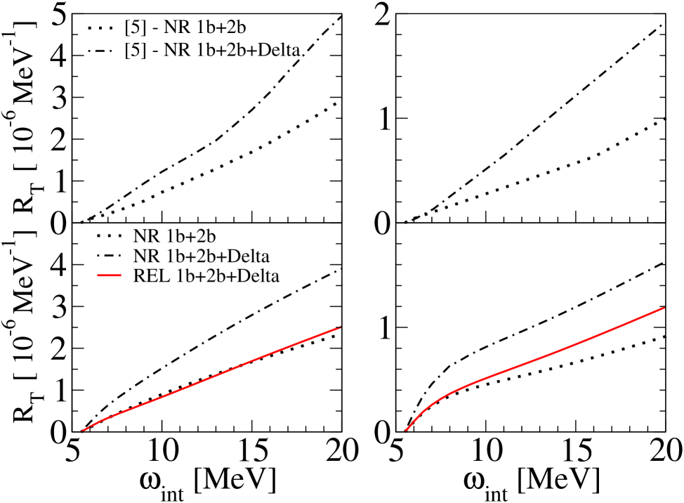
Figure 3: $R_{T}$ of ³He. Lower panels ($q=862$ MeV/c left, $q=927$ MeV/c right): theoretical result from present work with non-relativistic nucleon one-body current and MEC (dotted) and additional $\Delta$-IC dash-dotted, further addition of relativistic corrections for nucleon one-body current (solid). Upper panels ($q$ at threshold as in lower panels, but slightly varying with $\omega_{int}$, see text) : theoretical results from Deltuva et al. Deltuva1 with non-relativistic nucleon one-body current and MEC (dotted) and additional $\Delta$-contributions (dash-dotted).

Finally in Fig. 4 we compare the results of our calculation with experimental data Hi03 . Again, as in the calculation of Deltuva1 the momentum transfer is only quasi-constant. Therefore, in the left panel we show $R_{T}$ including all current contributions for the two extreme $q$ values, i.e. $q=862$ and $850$ MeV/c, and in addition for $q=862$ MeV/c the result where only $\Delta$-IC are left out. The lower $q$ corresponds to the data at about $\omega_{int}=20$ MeV, while the higher $q$ corresponds to the threshold energy. In the right panel of the figure we only show the results for $q=927$ MeV/c that corresponds to the data close to threshold. The $\Delta$-IC contribution is seen to be essential for obtaining a good agreement between theory and experiment below 10 MeV. However, at higher energies the increase due to $\Delta$-IC is not sufficient to describe the data even if one considers the slight shift of $q$ with higher energies represented by the dotted curve. The present case is rather similar to deuteron electrodisintegration at higher momentum transfer, where at low excitation energy the leading M1 transition also has a minimum. For the deuteron case it is known (see e.g. LeA83 ) that various theoretical ingredients, like for example the potential model dependence, can lead to rather large variations of the theoretical result. Thus our present study cannot give a final answer concerning the comparison of theory and experiment.

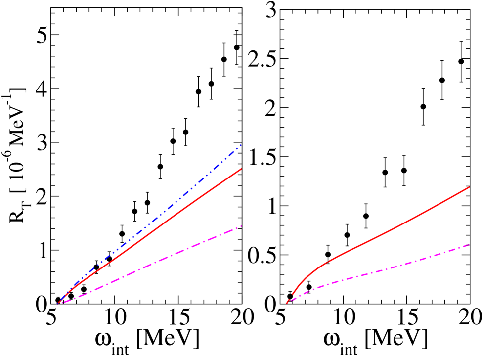
Figure 4: $R_{T}$ of ³He for same kinematics and the same dash-dotted and solid curves as in Fig. 2; in addition: result with all current contributions at $q=$ 850 MeV/c (dash-double dotted curve). Experimental data with slightly varying $q$-values from Hi03 .

We summarize our work as follows. We have illustrated how $\Delta$ degrees of freedom are integrated into the LIT formalism for a calculation of the inelastic inclusive transverse $(e,e^{\prime})$ response function $R_{T}$ of ³He. The resulting coupled equations for the Lorentz states of the $NNN$ and $NN\Delta$ channels contain, as opposed to the corresponding coupled Schrödinger equation, source terms with electromagnetic operators acting on the nuclear ground state. The $\Delta$ degrees of freedom are present in three different forms: (i) in the potentials $V^{N^{\prime}_{1}N^{\prime}_{2},N_{1}N_{2}}$, (ii) in the $\Delta$-propagator, and (iii) in the current operators ${\bf j}_{N^{\prime}_{1}N_{1}}$. The coupled channel equation is solved in impulse approximation, where the $NNN$ and $NN\Delta$ channels are treated separately. First, the $NNN$ part is solved using a realistic nuclear interaction with $NN$ and $NNN$ potentials. The result thus obtained is then used for the solution of the $NN\Delta$ channel. The former gives a contribution to the electrodisintegration of a purely nucleonic final state, whereas the latter leads to a contribution to the pion production channel. In the present work we have studied $\Delta$-effects in $R_{T}$ of ³He close to the breakup threshold at an momentum transfers of about 900 MeV/c. The response function is affected by sizable MEC contributions, and, as in a previous full coupled channel calculation Deltuva1 we find a considerable increase of $R_{T}$ due to $\Delta$ degrees of freedom. Unlike the calculation of Deltuva1 we here take into account relativistic corrections to the nonrelativistic one-body current operator. At the kinematics considered here these relativistic corrections nearly cancel the $\Delta$-IC contribution. This cancellation in fact leads to good agreement of our theoretical $R_{T}$ with experimental data at very low energy transfer, while the experimental $R_{T}$ is underestimated at somewhat higher energies.

V Acknowledgment

Acknowledgments of financial support are given to AuroraScience (L.P.Y.), to the RFBR, grant 10-02-00718 and RMES, grant NS-7235.2010.2 (V.D.E.), and to the National Science and Engineering Research Council of Canada (E.L.T.).

Appendix A Details of $g^{c},h^{c},g^{d},h^{d}$

The spin-isospin factors are

$$g^{c}_{B^{\prime}S^{\prime}T^{\prime},BS\mathcal{S}T\mathcal{T}}=\left\{\begin{array}[]{c@{\quad\quad}l}\frac{1}{\sqrt{2}}f_{B^{\prime}S^{\prime}T^{\prime},BS\mathcal{S}T\mathcal{T}}&\mbox{if $B^{\prime}=1$ and $B=0$, }\\ -(-)^{S+T}f_{B^{\prime}S^{\prime}T^{\prime},BS\mathcal{S}T\mathcal{T}}\Big{|}_{s_{1}\leftrightarrow s_{2},t_{1}\leftrightarrow t_{2}}&\mbox{if $B^{\prime}=0$ and $B=0$,}\\ 0&\mbox{otherwise.}\end{array}\right.$$ (32)

$$g^{d}_{B^{\prime}S^{\prime}T^{\prime},BS\mathcal{S}T\mathcal{T}}=\left\{\begin{array}[]{c@{\quad\quad}l}-(-1)^{S^{\prime}+T^{\prime}}\frac{1}{\sqrt{2}}f_{B^{\prime}S^{\prime}T^{\prime},BS\mathcal{S}T\mathcal{T}}\Big{|}_{s_{1}^{\prime}\leftrightarrow s_{2}^{\prime},t_{1}^{\prime}\leftrightarrow t_{2}^{\prime}}&\mbox{if $B^{\prime}=1$ and $B=0$, }\\ -(-)^{S^{\prime}+T^{\prime}}\sqrt{2}f_{B^{\prime}S^{\prime}T^{\prime},BS\mathcal{S}T\mathcal{T}}\Big{|}_{s_{1}^{\prime}\leftrightarrow s_{2}^{\prime},t_{1}^{\prime}\leftrightarrow t_{2}^{\prime}}&\mbox{if $B^{\prime}=0$ and $B=1$,}\\ 0&\mbox{otherwise.}\end{array}\right.$$ (33)

$$f_{B^{\prime}S^{\prime}T^{\prime},BS\mathcal{S}T\mathcal{T}}=(-)^{S+T}\hat{S^{\prime}}\hat{S}\hat{T^{\prime}}\hat{T}\left\{{s_{1}^{\prime}\;s_{2}^{\prime}\;S^{\prime}\atop s_{3}^{\prime}\;\mathcal{S}\;S}\right\}\left\{{t_{1}^{\prime}\;t_{2}^{\prime}\;T^{\prime}\atop t_{3}^{\prime}\;\mathcal{T}\;T}\right\}\delta_{s_{1}^{\prime}s_{3}}\delta_{s_{2}^{\prime}s_{1}}\delta_{s_{3}^{\prime}s_{2}}.$$ (34)

The spatial functions in coordinate representation are

$$\langle{\boldsymbol{\xi}}_{1}{\boldsymbol{\xi}}_{2}|h^{c}_{NK(Ll)\mathcal{LM_{L}}}\rangle=(-)^{L}\langle{\boldsymbol{\xi}}_{1}^{\prime}({\boldsymbol{\xi}}_{1},{\boldsymbol{\xi}}_{2}){\boldsymbol{\xi}}_{2}^{\prime}({\boldsymbol{\xi}}_{1},{\boldsymbol{\xi}}_{2})|h_{NK(Ll)\mathcal{LM_{L}}}\rangle,$$ (35)

$$\langle{\boldsymbol{\xi}}_{1}{\boldsymbol{\xi}}_{2}|h^{d}_{NK(Ll)\mathcal{LM_{L}}}\rangle=\langle{\boldsymbol{\xi}}_{1}^{\prime}(-{\boldsymbol{\xi}}_{1},{\boldsymbol{\xi}}_{2}){\boldsymbol{\xi}}_{2}^{\prime}(-{\boldsymbol{\xi}}_{1},{\boldsymbol{\xi}}_{2})|h_{NK(Ll)\mathcal{LM_{L}}}\rangle,$$ (36)

where ${\boldsymbol{\xi}}_{1}^{\prime}({\boldsymbol{\xi}}_{1},{\boldsymbol{\xi}}_{2})$ and ${\boldsymbol{\xi}}_{2}^{\prime}({\boldsymbol{\xi}}_{1},{\boldsymbol{\xi}}_{2})$ are connected to ${\boldsymbol{\xi}}_{1}$ and ${\boldsymbol{\xi}}_{2}$ through the cycle operator $(123)$ by $\left\langle{\bf r}_{1}^{\prime}{\bf r}_{2}^{\prime}{\bf r}_{3}^{\prime}s_{1}^{\prime}s_{2}^{\prime}s_{3}^{\prime}t_{1}^{\prime}t_{2}^{\prime}t_{3}^{\prime}\right|=\left\langle{\bf r}_{2}{\bf r}_{3}{\bf r}_{1}s_{2}s_{3}s_{1}t_{2}t_{3}t_{1}\right|$, and using (22) we have

$${\boldsymbol{\xi}}_{1}^{\prime}({\boldsymbol{\xi}}_{1},{\boldsymbol{\xi}}_{2}) = -\sqrt{\frac{A_{3}A_{1}}{(A_{2}+A_{3})(A_{1}+A_{2})}}\;{\boldsymbol{\xi}}_{1}+\sqrt{\frac{A_{2}(A_{1}+A_{2}+A_{3})}{(A_{2}+A_{3})(A_{1}+A_{2})}}\;{\boldsymbol{\xi}}_{2},$$

$${\boldsymbol{\xi}}_{2}^{\prime}({\boldsymbol{\xi}}_{1},{\boldsymbol{\xi}}_{2}) = -\sqrt{\frac{(A_{1}+A_{2}+A_{3})A_{2}}{(A_{2}+A_{3})(A_{1}+A_{2})}}\;{\boldsymbol{\xi}}_{1}-\sqrt{\frac{A_{1}A_{3}}{(A_{2}+A_{3})(A_{1}+A_{2})}}\;{\boldsymbol{\xi}}_{2}.$$ (37)

Appendix B Kinetic Energy Calculational Details

For a basis of antisymmetric states the kinetic energy can be written as

$$T=\frac{3}{2m_{N}}\frac{A_{1}+A_{2}}{A_{1}+A_{2}+A_{3}}{\boldsymbol{\pi}}^{2}_{1},$$ (38)

where ${\boldsymbol{\pi}}_{1}=-i\partial/\partial{\boldsymbol{\xi}}_{1}$ is the Jacobi momentum conjugate to ${\boldsymbol{\xi}}_{1}$. Noting that for calculating the matrix elements of ${\boldsymbol{\pi}}^{2}_{1}$ between the basis states (23) one may drop $\left(1-(12)\right)/\left[2(1+B^{\prime\prime 2})\right]^{1/2}$, we get

$$\langle\varphi_{k^{\prime}}|T|\varphi_{k}\rangle = \frac{3}{2m_{N}}\delta_{\mathcal{L^{\prime},L}}\delta_{\mathcal{S^{\prime},S}}\delta_{\mathcal{J^{\prime},J}}\delta_{\mathcal{M_{J^{\prime}},M_{J}}}\delta_{\mathcal{T^{\prime},T}}\delta_{\mathcal{M_{T^{\prime}},M_{T}}}\sum_{B"S"T"}\frac{A_{1}^{"}+A_{2}^{"}}{A_{1}^{"}+A_{2}^{"}+A_{3}^{"}}$$ (39)

$$\times\langle F_{B"S"T",B^{\prime}S^{\prime}\mathcal{S}T^{\prime}\mathcal{T}N^{\prime}K^{\prime}(L^{\prime}l^{\prime})\mathcal{LM_{L}}}|{\boldsymbol{\pi}}^{2}_{1}|F_{B"S"T",BS\mathcal{S}T\mathcal{T}NK(Ll)\mathcal{LM_{L}}}\rangle.$$

For the calculation of the spatial matrix elements we use the technique as described in Ef02 to get

$$\langle F_{j^{\prime}\mathcal{L^{\prime}M_{L^{\prime}}}}|{\boldsymbol{\pi}}^{2}_{1}|F_{j\mathcal{LM_{L}}}\rangle=\frac{\delta_{\mathcal{L^{\prime},L}}{\delta_{\mathcal{M_{L^{\prime}},M_{L}}}}8\pi^{2}}{2\mathcal{L}+1}\int d\tau_{int}\left\{\sum_{\mathcal{M"}}\left[\frac{\partial}{\partial\xi_{1}}\underline{F_{j^{\prime}\mathcal{LM"}}}\right]\left[\frac{\partial}{\partial\xi_{1}}\underline{F_{j\mathcal{LM"}}}\right]\right.$$

$$\left.+{\xi}^{-2}_{1}\sum_{{\mathcal{M"}},\mu=\pm}\underline{l_{\mu}F_{j^{\prime}\mathcal{LM"}}}\,\underline{l_{\mu}F_{j\mathcal{LM"}}}\right\},$$ (40)

where $d\tau_{int}={\xi}^{2}_{1}{\xi}^{2}_{2}d{\xi}_{1}d{\xi}_{2}dt,\;t=\hat{{\boldsymbol{\xi}}_{1}}\!\cdot\!\hat{{\boldsymbol{\xi}}_{2}}$. The underlines mean that the space points take the value

$$\xi_{1x}=0,\;\xi_{1y}=0,\;\xi_{1z}=\xi_{1},\;\xi_{2x}=\xi_{2}\sqrt{1-t^{2}},\;\xi_{2y}=0,\;\xi_{2z}=\xi_{2}t,\;$$ (41)

the orbital angular momentum is given by ${\bf l}={\boldsymbol{\xi}}_{1}\times{\boldsymbol{\pi}}_{1}$, and

$$\underline{l_{\pm 1}F_{j\mathcal{LM}}}=-\frac{\xi_{1}}{\sqrt{2}}\left[(\partial/\partial\xi_{1x})\pm i(\partial/\partial\xi_{1y})\right]F_{j\mathcal{LM}}$$ (42)

with the derivatives taken at the space point of (41).

Appendix C Calculational Details for $V(NN\to N\Delta)$ Potential

In calculating matrix elements of the transition potentials between antisymmetric basis states one may omit the factor $(1-(12))/\sqrt{(}2(1+B^{\prime 2})$ from Eq. (23) by using the substitutions

$$\frac{1-(12)}{\sqrt{2(1+B^{{}^{\prime}2})}}V^{N\Delta,NN}\rightarrow 3\cdot\sqrt{2}V_{12}(NN\rightarrow N\Delta),$$

$$V^{NN,N\Delta}\frac{1-(12)}{\sqrt{2(1+B^{2})}}\rightarrow 3\cdot\sqrt{2}V_{12}(N\Delta\rightarrow NN).$$

Each basis state in (23) is the sum of several terms of the form

$$\frac{1-(12)}{\sqrt{2(1+B^{{}^{\prime}2})}}\left|\left(F_{j\mathcal{L}}\otimes\left(\left(s_{1}^{\prime}s_{2}^{\prime}\right)S^{\prime}s_{3}^{\prime}\right)\mathcal{S}\right)_{\mathcal{JM_{J}}},\left(\left(t_{1}^{\prime}t_{2}^{\prime}\right)T^{\prime}t_{3}^{\prime}\right)\mathcal{TM_{T}}\right\rangle,$$

and this is also true for the basis of the $NNN$ part, but with $B=B^{\prime}=1,\;(s_{1},s_{2},s_{3})=(t_{1},t_{2},t_{3})=(1/2,1/2,1/2)$, and $\left(1-(12)\right)/\left[2(1+B^{\prime 2})\right]^{1/2}=1$. Therefore for the matrix elements of the operator $V_{12}$ we need

$$\left\langle\left(F_{j^{\prime}\mathcal{L^{\prime}}}\otimes\left(\left(s_{1}^{\prime}s_{2}^{\prime}\right)S^{\prime}s_{3}^{\prime}\right)\mathcal{S^{\prime}}\right)_{\mathcal{J^{\prime}M_{J^{\prime}}}}\right|V_{0}(m_{B}){\boldsymbol{\sigma}}_{1}\!\cdot\!{\boldsymbol{\sigma}}_{2}\left|\left(F_{j\mathcal{L}}\otimes\left(\left(s_{1}s_{2}\right)Ss_{3}\right)\mathcal{S}\right)_{\mathcal{JM_{J}}}\right\rangle$$

$$=-\delta_{\mathcal{L^{\prime},L}}\delta_{S^{\prime},S}\delta_{s_{3}^{\prime},s_{3}}\delta_{\mathcal{S^{\prime},S}}\delta_{\mathcal{J^{\prime},J}}\delta_{\mathcal{M_{J^{\prime}},M_{J}}}\frac{1}{\hat{{\mathcal{L}}}}\langle{F_{j^{\prime}\mathcal{L}}}||V_{0}(m_{B})||{F_{j\mathcal{L}}}\rangle$$

$$\times(-1)^{1+S^{\prime}+s_{1}+s_{2}^{\prime}}\left\{{s_{1}^{\prime}\;s_{1}\;1\atop s_{2}\;s_{2}^{\prime}\;S^{\prime}}\right\}\langle s_{1}^{\prime}||\sigma_{1}||s_{1}\rangle\langle s_{2}^{\prime}||\sigma_{2}||s_{2}\rangle.$$ (43)

In the spatial matrix elements entering here we note that the $NNN$ component and the $NN\Delta$ component of the wave function are given in terms of the Jacobi vectors of the same form (22) but with different mass numbers. To perform the integration one needs to express one set of the Jacobi vectors in terms of the other via

$$\overline{{\boldsymbol{\xi}}}_{1}({\boldsymbol{\xi}}_{1},{\boldsymbol{\xi}}_{2}) = \sqrt{\frac{A_{2}^{\prime}A_{1}^{\prime}(A_{1}+A_{2})}{(A_{1}^{\prime}+A_{2}^{\prime})A_{1}A_{2}}}\;{\boldsymbol{\xi}}_{1}$$

$$\overline{{\boldsymbol{\xi}}}_{2}({\boldsymbol{\xi}}_{1},{\boldsymbol{\xi}}_{2}) = \frac{(A_{1}^{\prime}A_{2}-A_{2}^{\prime}A_{1})}{\sqrt{A^{\prime}(A_{1}^{\prime}+A_{2}^{\prime})A_{1}A_{2}(A_{1}+A_{2})}}\;{\boldsymbol{\xi}}_{1}+\sqrt{\frac{(A_{1}^{\prime}+A_{2}^{\prime})A_{3}^{\prime}A}{A^{\prime}(A_{1}+A_{2})A_{3}}}\;{\boldsymbol{\xi}}_{2},$$ (44)

where $A^{\prime}=A_{1}^{\prime}+A_{2}^{\prime}+A_{3}^{\prime},\;A=A_{1}+A_{2}+A_{3}.$ The integration is done as

$$\langle{F_{j^{\prime}\mathcal{L}}}||V_{0}(m_{B})||{F_{j\mathcal{L}}}\rangle=8\pi^{2}(2\mathcal{L}+1)^{-1/2}\int d\tau_{int}\sum_{\mathcal{M}}\underline{F_{j^{\prime}\mathcal{LM}}}(\overline{{\boldsymbol{\xi}}}_{1},\overline{{\boldsymbol{\xi}}}_{2})V_{0}(m_{B})\underline{F_{j\mathcal{LM}}}({\boldsymbol{\xi}}_{1},{\boldsymbol{\xi}}_{2}).$$ (45)

In addition we need ( using ${\mathcal{N}}^{(2)}_{M}=4(\pi/5)^{1/2}Y_{2M}({\bf n})$)

$$\left\langle\left(F_{j^{\prime}\mathcal{L^{\prime}}}\otimes\left(\left(s_{1}^{\prime}s_{2}^{\prime}\right)S^{\prime}s_{3}^{\prime}\right)\mathcal{S^{\prime}}\right)_{\mathcal{J^{\prime}M_{J^{\prime}}}}\right|V_{2}(m_{B})S_{12}\left|\left(F_{j\mathcal{L}}\otimes\left(\left(s_{1}s_{2}\right)Ss_{3}\right)\mathcal{S}\right)_{\mathcal{JM_{J}}}\right\rangle$$

$$\;\;\;\;=\delta_{\mathcal{J^{\prime},J}}\delta_{\mathcal{M_{J^{\prime}},M_{J}}}(-1)^{{\mathcal{L+S^{\prime}+J^{\prime}}}}{3}/{2}\left\{{\mathcal{L^{\prime}}\;\mathcal{L}\;2\atop\mathcal{S}\;\mathcal{S^{\prime}}\;\mathcal{J^{\prime}}}\right\}\langle{F_{j^{\prime}\mathcal{L^{\prime}}}}||V_{2}(m_{B}){\mathcal{N}}^{(2)}||{F_{j\mathcal{L}}}\rangle$$

$$\;\;\;\qquad\times\langle\left(\left(s_{1}^{\prime}s_{2}^{\prime}\right)S^{\prime}s_{3}^{\prime}\right)\mathcal{S^{\prime}}||\Sigma^{(2)}||\left(\left(s_{1}s_{2}\right)Ss_{3}\right)\mathcal{S}\rangle,$$ (46)

$$\langle{F_{j^{\prime}\mathcal{L^{\prime}}}}||V_{2}(m_{B}){\mathcal{N}}^{(2)}||{F_{j\mathcal{L}}}\rangle\\ =16\pi^{2}(2\mathcal{L^{\prime}}+1)^{-1/2}\int d\tau_{int}\sum_{\mathcal{M}}C^{\mathcal{L^{\prime}M}}_{\mathcal{LM}20}\underline{F_{j^{\prime}\mathcal{L^{\prime}M}}}(\overline{{\boldsymbol{\xi}}}_{1},\overline{{\boldsymbol{\xi}}}_{2})V_{2}(m_{B})\underline{F_{j\mathcal{LM}}}({\boldsymbol{\xi}}_{1},{\boldsymbol{\xi}}_{2}),$$

and

$$\langle\left(\left(s_{1}^{\prime}s_{2}^{\prime}\right)S^{\prime}s_{3}^{\prime}\right)\mathcal{S^{\prime}}||\Sigma^{(2)}||\left(\left(s_{1}s_{2}\right)Ss_{3}\right)\mathcal{S}\rangle$$

$$=\delta_{s_{3}^{\prime},s_{3}}(-1)^{S^{\prime}+s_{3}^{\prime}+{\mathcal{S}}}\sqrt{30}/{3}\hat{S^{\prime}}\hat{S}\hat{\mathcal{S^{\prime}}}\hat{\mathcal{S}}\left\{{\mathcal{S^{\prime}}\;\mathcal{S}\;2\atop{S}\;{S^{\prime}}\;{s_{3}^{\prime}}}\right\}\left\{\begin{array}[]{ccc}s_{1}^{\prime}&s_{1}&1\\ s_{2}^{\prime}&s_{2}&1\\ S^{\prime}&S&2\end{array}\right\}\langle s_{1}^{\prime}||\sigma_{1}||s_{1}\rangle\langle s_{2}^{\prime}||\sigma_{2}||s_{2}\rangle.$$ (50)

Appendix D $T_{jm}^{l}$ Multipoles of One-Body Currents Relating $\Delta$

For the magnetic multipoles one has

$${T}^{j}_{jm}=\sum_{i}[{T}^{j,\,{\rm spin}}_{jm}(i)+{T}^{j,\,{\rm conv}}_{jm}(i)].$$ (51)

we have

$$\!\!\!\!{T}^{j,\,{\rm spin}}_{\Delta N,jm}(i)=\frac{1}{m_{\Delta}}\frac{q}{2}\overline{\mu}^{\Delta N}_{p}\tau_{zi}\left\{\sqrt{\frac{j}{2j+1}}j_{j+1}(qr^{\prime}_{i})[Y_{j+1}(\hat{\mathbf{r}}^{\prime}_{i})\otimes\sigma_{i}]_{jm}\right.$$

$$\!\!\!\!\!\!\!\left.-\sqrt{\frac{j+1}{2j+1}}j_{j-1}(qr^{\prime}_{i})[Y_{j-1}(\hat{\mathbf{r}}^{\prime}_{i})\otimes\sigma_{i}]_{jm}\right\},$$ (52)

$$\!\!\!\!{T}^{j,\,{\rm spin}}_{\Delta\Delta,jm}(i)=\frac{1}{m_{\Delta}}\frac{q}{2}{\bar{\mu}}^{\Delta}_{p}\left(\frac{1}{2}+\frac{1}{2}\tau_{zi}\right)\left\{\sqrt{\frac{j}{2j+1}}j_{j+1}(qr^{\prime}_{i})[Y_{j+1}(\hat{\mathbf{r}}^{\prime}_{i})\otimes\sigma_{i}]_{jm}\right.$$

$$\!\!\!\!\!\!\!\left.-\sqrt{\frac{j+1}{2j+1}}j_{j-1}(qr^{\prime}_{i})[Y_{j-1}(\hat{\mathbf{r}}^{\prime}_{i})\otimes\sigma_{i}]_{jm}\right\},$$ (53)

$${T}^{j,{\rm conv}}_{\Delta\Delta,jm}(i)=\frac{1}{m_{\Delta}}\left(\frac{1}{2}+\frac{1}{2}\tau_{zi}\right)j_{j}(qr^{\prime}_{i})\left[Y_{j}(\hat{\mathbf{r}}^{\prime}_{i})\otimes\partial^{\prime}_{i}\right]_{jm}.$$ (54)

The quantity $\partial^{\prime}_{\mu}$ is defined by the relationship $-i\partial^{\prime}_{\mu}=p^{\prime}_{\mu}$, and

$$\partial^{\prime(3)}_{\mu}=\left[\frac{(A_{1}+A_{2})A_{3}}{A}\right]^{1/2}\frac{\partial}{\partial\xi_{2,\mu}}.$$

For the electric multipoles

$$T^{l}_{jm}=\sum_{i}[T^{l,\,{\rm spin}}_{jm}(i)+T^{l,\,{\rm conv}}_{jm}(i)]$$ (55)

where $l=j\pm 1$. One obtains

$$T^{j\pm 1,\,{\rm spin}}_{\Delta N,jm}(i)=-\frac{1}{m_{\Delta}}\frac{q}{2}\overline{\mu}^{\Delta N}_{p}\tau_{zi}\sqrt{\frac{j+(1\mp 1)/2}{2j+1}}j_{j}(qr^{\prime}_{i})\left[Y_{j}(\hat{\mathbf{r}}_{i}^{\prime})\otimes\sigma_{i}\right]_{jm}$$ (56)

$$T^{j\pm 1,\,{\rm spin}}_{\Delta\Delta,jm}(i)=-\frac{1}{m_{\Delta}}\frac{q}{2}{\bar{\mu}}^{\Delta}_{p}\left(\frac{1}{2}+\frac{1}{2}\tau_{zi}\right)\sqrt{\frac{j+(1\mp 1)/2}{2j+1}}j_{j}(qr^{\prime}_{i})\left[Y_{j}(\hat{\mathbf{r}}_{i}^{\prime})\otimes\sigma_{i}\right]_{jm}$$ (57)

$$T^{j\pm 1,\,{\rm conv}}_{\Delta\Delta,jm}(i)=\pm\frac{1}{m_{\Delta}}\left(\frac{1}{2}+\frac{1}{2}\tau_{zi}\right)\left\{j_{j\pm 1}(qr^{\prime}_{i})\left[Y_{j\pm 1}(\hat{\mathbf{r}}^{\prime}_{i})\otimes\partial^{\prime}_{i}\right]_{jm}\right.$$

$$\left.-\kappa\frac{q}{2}\sqrt{\frac{j+(1\pm 1)/2}{2j+1}}j_{j}(qr^{\prime}_{i})Y_{jm}(\hat{\mathbf{r}}^{\prime}_{i})\right\}.$$ (58)

For the combined $r$- and spin space operator we only need the reduced matrix element for the calculation of the response function, as seen in (28). The reduced matrix element is given by

$$\left\langle\left(F_{j^{\prime}\mathcal{L^{\prime}}}\otimes\left(\left(s_{1}^{\prime}s_{2}^{\prime}\right)S^{\prime}s_{3}^{\prime}\right)\mathcal{S^{\prime}}\right)_{\mathcal{J^{\prime}}}\right\|(O_{l}\otimes O_{s})_{j}\left\|\left(F_{j\mathcal{L}}\otimes\left(\left(s_{1}s_{2}\right)Ss_{3}\right)\mathcal{S}\right)_{\mathcal{J}}\right\rangle$$

$$=\hat{\mathcal{J^{\prime}}}\hat{\mathcal{J}}\hat{j}\left\{\begin{array}[]{ccc}{\mathcal{L^{\prime}}}&{\mathcal{L}}&l\\ {\mathcal{S^{\prime}}}&{\mathcal{S}}&s\\ {\mathcal{J^{\prime}}}&{\mathcal{J}}&j\end{array}\right\}\langle{F_{j^{\prime}\mathcal{L^{\prime}}}}||O_{l}||{F_{j\mathcal{L}}}\rangle\langle\left(\left(s_{1}^{\prime}s_{2}^{\prime}\right)S^{\prime}s_{3}^{\prime}\right)\mathcal{S^{\prime}}||O_{s}||\left(\left(s_{1}s_{2}\right)Ss_{3}\right)\mathcal{S}\rangle,$$ (62)

where

$$\langle{F_{j^{\prime}\mathcal{L^{\prime}}}}||O_{l}||{F_{j\mathcal{L}}}\rangle\\ =8\pi^{2}(2\mathcal{L^{\prime}}+1)^{-1/2}\int d\tau_{int}\sum_{{\mathcal{M}}m}C^{{\mathcal{L^{\prime}(M}}+m)}_{\mathcal{LM}lm}\underline{F_{j^{\prime}\mathcal{L^{\prime}M}}}(\overline{{\boldsymbol{\xi}}}_{1},\overline{{\boldsymbol{\xi}}}_{2})\underline{O_{l}F_{j\mathcal{LM}}}({\boldsymbol{\xi}}_{1},{\boldsymbol{\xi}}_{2}),$$

and $O_{l}$ is a function of relative coordinate and momentum

$${\bf r}_{3}-{\bf R}_{cm}=\left[\frac{(A_{1}+A_{2})}{AA_{3}}\right]^{1/2}{\boldsymbol{\xi}}_{2},\qquad i\left({\bf p}_{3}-\frac{A_{3}}{A}{\bf P}_{cm}\right)=\left[\frac{(A_{1}+A_{2})A_{3}}{A}\right]^{1/2}\frac{\partial}{\partial{\boldsymbol{\xi}}_{2}}.$$

References

• (1) M.Rho and D.H.Wilkinson,eds,Mesons in Nuclei, North-Holland, Amsterdam 1979.
• (2) H. Arenhövel, W. Leidemann, and E. L. Tomusiak, Eur. Phys. J. A 23, 147 (2005).
• (3) M. Viviani, A. Kievsky, L. E. Marcucci, S. Rosati and R. Schiavilla, Phys. Rev. C 61, 064001 (2000).
• (4) J. Golak, R. Skibinski, H. Witala, W. Glöckle, A. Nogga and H. Kamada, Phys. Rept. 415, 89 (2005).
• (5) A. Deltuva, L.P. Yuan, J. Adam, and P.U. Sauer, Phys. Rev. C 70, 034004 (2004).
• (6) S. Della Monaca, V.D. Efros, A. Khugaev, W. Leidemann, G. Orlandini, E.L. Tomusiak and L.P. Yuan, Phys. Rev. C 77, 044007 (2008).
• (7) W. Leidemann, V.D. Efros, G. Orlandini and E.L. Tomusiak, Few-Body Systems 47, 157 (2010).
• (8) L. P. Yuan, K. Chmielewski, M. Oelsner, P. U. Sauer, and J. Adam, Jr, Phys. Rev. C 66,054004 (2002).
• (9) A. Deltuva, L.P. Yuan, J. Adam, A.C. Fonseca and P.U. Sauer, Phys. Rev. C 69,034004 (2004).
• (10) R. Schiavilla, R. B. Wiringa, V. R. Pandharipande, and J. Carlson, Phys. Rev. C 45, 2628 (1992).
• (11) H.J. Weber and H. Arenhövel, Phys. Rep. C 36, 277 (1978).
• (12) W. Leidemann and H. Arenhövel, Nucl. Phys. A465, 573 (1987).
• (13) V.D. Efros, W. Leidemann and G. Orlandini, Phys. Lett. B338, 130 (1994).
• (14) V.D. Efros, W. Leidemann, G. Orlandini and N. Barnea, J. Phys. G 34, R459 (2007).
• (15) V.D. Efros, W. Leidemann, G. Orlandini and E.L. Tomusiak, Phys. Rev. C 69, 044001 (2004).
• (16) S. Bacca, N. Barnea, W. Leidemann, and G. Orlandini, Phys. Rev. Lett. 102, 162501 (2009); Phys. Rev. C 80, 064001 (2009).
• (17) V.D. Efros, W. Leidemann, G. Orlandini and E.L. Tomusiak, Phys. Rev. C 72, 011002(R) (2005).
• (18) V.D. Efros, W. Leidemann, G. Orlandini and E.L. Tomusiak, Phys. Rev. C 81, 034001 (2010).
• (19) S. Bacca, H. Arenhövel, N. Barnea, W. Leidemann and G. Orlandini, Phys. Rev. C 76, 014003 (2007).
• (20) R.B. Wiringa, V.G.J. Stoks and R. Schiavilla, Phys. Rev. C 51, 38 (1995).
• (21) B.S. Pudliner, V.R. Pandharipande, J. Carlson, S.C. Pieper and R.B. Wiringa, Phys. Rev. C 56, 1720 (1997).
• (22) H. Arenhövel and M. Schwamb, Eur.Phys.J. A12, 207 (2001).
• (23) M. A. Marchisio, N. Barnea, W. Leidemann and G. Orlandini, Few-Body Syst. 33, 259 (2003).
• (24) N. Barnea, V.D. Efros, W. Leidemann and G. Orlandini, Few-Body Syst. 47, 210 (2010).
• (25) D. Andreasi, W. Leidemann, Ch. Reiss and M. Schwamb, Eur. Phys. J. A 24, 361 (2005).
• (26) A. Deltuva, R. Machleidt, and P. U. Sauer, Phys. Rev. C 68, 024005 (2003).
• (27) S. Galster et al., Nucl. Phys. B32, 221 (1971).
• (28) R. Machleidt, Phys. Rev. C 63, 024001 (2001).
• (29) R.S. Hicks et al, Phys. Rev. C 67, 064004 (2003).
• (30) V.D. Efros, Few-Body Syst. 32, 169 (2002).
• (31) W. Leidemann and H. Arenhövel, Nucl. Phys. A393, 385 (1983).