Scattering of charge carriers in graphene induced by topological defects

Abstract

We study the scattering of graphene quasiparticles by topological defects, represented by holes, pentagons and heptagons. For the case of holes, we obtain the phase shift and found that at low concentration they appear to be irrelevant for the electron transport, giving a negligible contribution to the resistivity. Whenever pentagons are introduced into the lattice and the fermionic current is constrained to move near one of them we realize that such a current is scattered with an angle that depends only on the number of pentagons and on the side the current taken. Such a deviation may be determined by means of a Young-type experiment, through the interference pattern between the two current branches scattered by a pentagon. In the case of a heptagon such a current is also scattered but it diverges from the defect, preventing a interference between two beams of current for the same heptagon.

I Introduction and Motivation

Graphene is a flat monolayer of carbon atoms tightly packed into a two-dimensional ($2D$) honeycomb lattice, (Fig. 1) or it can be viewed as an individual atomic plane pulled out of bulk graphite Novoselov04 ; Novoselov05 . It is the first example of a truly atomic two-dimensional $(2D)$ crystalline system and it is the basic building blocks for graphitic materials such as fullerenes (graphene balled into a sphere) or carbon nanotubes (graphene rolled-up in cylinders) Geim07 ; Castro-Neto06 ; Geim08 . Additionally, it is a zero-gap semiconductor, in which the low energy spectrum is correctly described by the $(2+1)D$ Dirac-like equation for a massless particle Novoselov05 ; Katsnelson06 ; Wallace47

$$i\hbar\frac{\partial}{\partial t}|\Psi\rangle=v_{F}\vec{\sigma}\cdot\vec{p}|\Psi\rangle,$$ (1)

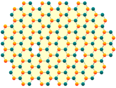
Figure 1: (Color online) Graphene is a flat monolayer of carbon atoms having a honeycomb lattice, consisting of two interpenetrating triangular sublattices (green and red circles). Experimental techniques provide high-quality graphene crystallites up to $100\mu m$ in size, which is sufficient for most research purpose, including the ones considered here. In this “perfect” layer the charge carries can travel thousands of interatomic distances without scattering.

where $v_{F}$ is the Fermi velocity, which plays the role of the speed of light ($v_{F}\approx c/300$), $\vec{\sigma}=(\sigma_{x},\sigma_{y})$ are the $2D$ Pauli matrices, $\vec{p}=-i\hbar\vec{\nabla}$ is the linear momentum operator and $|\Psi\rangle$ is a two-component spinor. Therefore, the quasiparticles can be viewed as electrons that have lost their masses or as (massless) neutrinos that acquired the electronic charge. Such a spectrum makes graphene a material with unique electronic properties. Its description by means of the Dirac equation is a direct consequence of graphene?s crystal symmetry. Its honeycomb lattice is made up of two equivalent triangular carbon sublattices $A$ and $B$, whereas its cosine-like energy bands associated with the sublattices intersect at zero energy $(E=0)$ near the edges of the Brillouin zone, giving rise to a conical section spectrum at low energiesGeim07 , say, $|E|\,<\,1$ eV. In this honeycomb lattice, the two-component spinor $|\Psi\rangle$ is referred to as pseudospin since it is an index indicating two interpenetrating triangular sublattices $A$ e $B$, which is similar to spin index (up and down) in quantum electrodynamics (QED). It is common to regard the sublattice degree of freedom as a pseudospin, with the $A$ sublattice being the “up”, $|+\rangle$ and $B$ sublattice being the “down”, $|-\rangle$, i.e.,

$$|+\rangle=\left(\begin{array}[]{cc}1\\ 0\\ \end{array}\right);\qquad|-\rangle=\left(\begin{array}[]{cc}0\\ 1\\ \end{array}\right).$$ (6)

Since $v_{F}\ll c$, it is a slow relativistic system or a strong coupling version of QED since the graphene’s dimensionless coupling constant, $e^{2}/\hbar v_{F}\approx 1$ much higher than its QED analogue, the fine structure constant $e^{2}/\hbar c\approx 1/137$. All these properties make the graphene a very interesting system, which provides a way to probe QED phenomena, for instance, by measuring its electronic properties. Several proposals for testing some predicted, but not yet observed phenomena in QED, including the Klein paradox Katsnelson06 ; Katsnelson07 , vacuum polarization Shytov07 and atomic collapse Shytov+07 , are some topics under investigation in graphene.

Here, we would like to study the behavior of graphene quasiparticles in the presence of defects in the crystalline structure of the material. We shall consider three types of defects: holes, pentagons and heptagons. All these defects can be incorporated by removing or inserting a few carbon atoms. Understanding how these defects modify the transport properties of graphene is crucial to achieve future electronic devices using carbon-made materials.

The presence of defects like pentagons (heptagons) induces positive (negative) curvature in the material. At some extent the charge carriers motion in the presence of pentagonal (heptagonal) defects is identical to fermions moving in a $(2+1)D$ gravitational space-time generated by positive (“negative”) point-like masses. Then we may employ results from gravity to analyze some effects concerning charge carriers in the presence of such defects. For instance, in the presence of pentagons and heptagons we found that the phase shifts of the carriers moving near these defects depend only on the number of pentagons or heptagons in the graphene sheet and are identical for charge carriers in the sublattice $A$ or $B$. In the case of the holes we computed the phase shifts for the scattered electrons and found that at low concentration they are irrelevant for the electrons transport giving no appreciable contribution to the resistivity.

II Charge carriers dynamics in a non-simply connected graphene sheet

In this section we discuss the scattering of the charge carriers in a non-simply connected graphene sheet. In the continuum model for the graphene, it is assumed that there is a hole of radius $r_{0}$ cut from the system center, located at the origin. Thus the motion of the quasiparticles is performed on a flat $2D$ support given by a non-simply connected manifold, which can be viewed as defect in the material. This model allows for the investigation of scattering effects as a function of the hole radius and could shed some light on the high charge carrier mobilities, fact observed in graphene Novoselov05 ; Katsnelson08 . In addition, it is interesting to compare our results with the scattering by a short-range potential because it appears that in the case of graphene the contribution of such small defects to the resistivity is essentially smaller than for conventional nonrelativistic two-dimensional electron gas Katsnelson07 ; Katsnelson08 .

To determine the phase-shift of the scattered wave function as well as the scattering cross section one has to solve the two-dimensional Dirac equation (1) which, for the case of massless particles, can be writing in a covariant form,like below:

$$i\hbar\gamma^{\mu}\partial_{\mu}\psi(x)\,=\,0,$$ (7)

where the covariant derivative is $\partial_{\mu}=[(1/v_{F})\partial/\partial t\,,\,\partial/\partial x\,,\,\partial/\partial y\,]$, the $\gamma$-matrices are $\gamma^{0}=\sigma^{3},$ $\gamma^{1}=i\sigma^{2}$ and $\gamma^{3}=-i\sigma^{1},$ obeying $\gamma^{\mu}\gamma^{\nu}=\eta^{\mu\nu}-i\epsilon^{\mu\nu\alpha}\gamma_{\alpha}$, $\eta^{\mu\nu}$ is the Minkowski tensor metric, ${\rm diag}(\eta^{\mu\nu})=(+1,-1,-1)$ and $\epsilon^{\mu\nu\alpha}$ is the 3-dimensional Levi-Civita symbol $(\epsilon^{012}\equiv+1).$ (The word covariant must be used carefully because $v_{F}$ is not invariant, being only a parameter and the term covariant is used to refer only the form the equation is written.) We may expand the solutions of the free massless Dirac equation in plane waves, once rotational invariance allows to separate the $\theta$ variable, so that the diagonalized angular momentum $\mathcal{J}=-i\hbar\frac{\partial}{\partial\theta}+\frac{\hbar}{2}\sigma^{3}$, yielding partial waves with angular momentum $(n+\frac{1}{2})\hbar$, takes the form,

$$\psi(\vec{r},t)=e^{i(n+\frac{1}{2}-\frac{1}{2}\sigma^{3})\theta}u_{n}(r)e^{-iEt/\hbar}.$$ (8)

The components of the radial spinor $u_{n}(r)$, given by $f_{n}(r)$ and $g_{n}(r)$, satisfy the Bessel equation of order $n$ and $n+1$, say:

$$\frac{d^{2}f_{n}(r)}{dr^{2}}+\frac{1}{r}\frac{df_{n}(r)}{dr}+\bigg{(}k^{2}-\frac{n^{2}}{r^{2}}\bigg{)}f_{n}(r)\,=0\,,$$ (9)

$$\frac{d^{2}g_{n}(r)}{dr^{2}}+\frac{1}{r}\frac{dg_{n}(r)}{dr}+\bigg{(}k^{2}-\frac{(n+1)^{2}}{r^{2}}\bigg{)}g_{n}(r)\,=0\,,$$ (10)

where $n\,=\,0\,,\pm 1\,,\pm 2\,,\ldots$ is the angular-momentum number and $k=\frac{E}{\hbar v_{F}}>0\,$ (we are considering only solutions with $E>0$ that describe the electronic dynamics). Remember that the spinor index in graphene labels its two crystal sublattices rather than directions of the actual spin. The solution for the radial spinor outside of the hole (i.e., for $r>r_{0}$) is given by:

$$u_{n}(r) = \left(\begin{array}[]{c}f_{n}(r)\\ g_{n}(r)\end{array}\right)$$ (13)

$$= \left(\begin{array}[]{c}B_{1n}\,J_{n}(kr)+B_{2n}\,N_{n}(kr)\\ B_{3n}\,J_{n+1}(kr)+B_{4n}\,N_{n+1}(kr)\\ \end{array}\right),$$ (16)

where $J_{n}$ and $N_{n}$ are the Bessel functions of first and second kinds (Neumann function), respectively, whereas $B_{jn}\,\,(j\,=1\,,\,2\,,\,3\,,\,4)$ are constants. These constants must be determined by the appropriate boundary conditions specified to completely define the problem. From the physical point of view, the correct boundary condition is determined by the requirement of vanishing the net energy flux into the hole, which is a region absent of lattice degrees of freedom. Consequently, the fields must arrange themselves in such a way that the energy flux from the incoming modes (asymptotically behaving like $e^{-ikr}$) exactly cancel that from the outgoing waves.

Let us recall that in the case without a hole, one has:

$$u_{n}(r)=\left(\begin{array}[]{c}B_{1n}\,J_{n}(kr)\\ B_{3n}\,J_{n+1}(kr)\\ \end{array}\right).$$ (17)

To determine the phase-shift $\delta_{n}$, we need the asymptotic behavior, $r\rightarrow\infty$, of the radial spinor (17) sayMorse Feshback :

$$u_{n}^{A}(r)\Big{|}_{r\rightarrow\infty}\longrightarrow\sqrt{\frac{2}{\pi kr}}\cos\bigg{(}kr-\frac{n\pi}{2}-\frac{\pi}{4}+\delta_{n}^{A}\bigg{)}\,,$$

$$u_{n}^{B}(r)\Big{|}_{r\rightarrow\infty}\longrightarrow\sqrt{\frac{2}{\pi kr}}\cos\bigg{(}kr-\frac{(n+1)\pi}{2}-\frac{\pi}{4}+\delta_{n}^{B}\bigg{)}\,,$$ (18)

where the spinor indices $A$ and $B$ labels the two crystal sublattices. Now, imposing Neumann boundary condition (NBC) on the wave-functions, $\frac{\partial u_{n}}{\partial r}\Big{|}_{r=r_{0}}=0$, we obtain:

$$u_{n}(r)=\left(\begin{array}[]{c}B_{1n}\big{[}J_{n}(kr)-\tan(t_{n}(kr_{0}))N_{n}(kr)\big{]}\\ B_{3n}\big{[}J_{n+1}(kr)-\tan(t_{n+1}(kr_{0}))N_{n+1}(kr)\big{]}\\ \end{array}\right)\,,$$ (19)

where

$$\tan[t_{n}(kr_{0})]=\frac{J^{\prime}_{n}(kr_{0})}{N^{\prime}_{n}(kr_{0})}\,,$$ (20)

The terms proportional to Bessel (Neumann) functions describe the incident (scattered) waves. Comparing their asymptotic behavior with those for plane waves, eq. (II), we obtain the phase shifts. Asymptotically, the scattered wave-function $u_{n}(r)$ behaves like follows:

$$u_{n}^{A}(r)\Big{|}_{r\rightarrow\infty} \longrightarrow \sqrt{\frac{2}{\pi kr}}\cos\Big{(}kr-\frac{n\pi}{2}-\frac{\pi}{4}+t_{n}(kr_{0})\Big{)}\,,$$

$$u_{n}^{A}(r)\Big{|}_{r\rightarrow\infty} \longrightarrow \sqrt{\frac{2}{\pi kr}}\cos\Big{(}kr-\frac{(n+1)\pi}{2}-\frac{\pi}{4}+t_{n+1}(kr_{0})\Big{)}\,,$$ (21)

giving us the phase-shift $\delta_{n}$ of the n-th partial wave that completely determines the fermionic scattering:

$$\delta_{n}^{A}=t_{n}(kr_{0})\,,$$ (22)

$$\delta_{n}^{B}=t_{n+1}(kr_{0})\,.$$ (23)

Now, if we consider a small concentration of point-like defects with concentration $n_{\rm def}$ angle-depedent scattering cross section, $\sigma(\theta),$ their contribution to resistivity, $\rho$, reads Katsnelson07 :

$$\rho = \frac{2}{e^{2}v_{F}^{2}N(E_{F})\tau(k_{F})}\,,$$

$$\frac{1}{\tau(k_{F})} = n_{\rm def}v_{F}\int_{0}^{2\pi}d\theta\frac{d\sigma(\theta)}{d\theta}(1-\cos\theta)\,,$$ (24)

where $N(E_{F})=2k_{F}/\pi\hbar v_{F}$ is the density of states at the Fermi level, taking into account the four-fold degeneracy, the spin and valley of the graphene, and $\tau$ is the mean-free path. For electrons of the sublattice $A$ we have:

$$\frac{d\sigma(\theta)}{d\theta}=\frac{2}{\pi k}\Bigg{|}\sum_{n=-\infty}^{n=\infty}t_{n}(kr_{0})e^{i\theta}\Bigg{|}^{2}\,.$$ (25)

The Dirac eq. (7) or (9) has an important symmetry under the interchanging $f\longleftrightarrow g\,,\,n\longleftrightarrow-n-1$ which implies that $t_{n}=t_{-n-1}$. Thus, eq. (25) can be written in the form:

$$\frac{d\sigma(\theta)}{d\theta}=\frac{2}{\pi k}\Bigg{|}\sum_{n=0}^{n=\infty}t_{n}(kr_{0})\cos[(n+1/2)\theta]\Bigg{|}^{2}\,.$$ (26)

For small energies, $kr_{0}\ll 1$, which is typical for graphene, one has

$$\delta_{n}^{A}=t_{n}(kr_{0})\simeq\frac{(2n+1)[(2n+3)n-(kr_{0})^{2}]}{[(2n+1)!!]^{2}(2n+3)(n+1)}(kr_{0})^{2n+1}$$ (27)

and thus the s-scattering $(n=0)$ dominates. With eqs. (26-27) the impurities contribution to the resistivity may be estimated as

$$\rho\simeq n_{\rm def}\frac{h}{e^{2}kk_{F}}(kr_{0})^{6}\,.$$ (28)

This means that the scattering induced by small holes (with radius around a few angstroms; some lattice spacings) at low concentration are irrelevant for the electronic transport in graphene, giving a negligible contribution to the resistivity. For the case of a potential $V(r)=V_{0}$ at $r<R_{0}$ and $V(r)=0$ at $r>R_{0},$ the estimation for this type of impurity contribution to the resistivity isKatsnelson07 $\rho\simeq(h/4e^{2})n_{\rm def}R_{0}^{2}$, giving a negligible contribution to the resistivity when the radius of the potential $R_{0}$ is of the order of interatomic distances and at a low concentration as above.

For an intuitive understanding of the result (28) let us recall that light does not experience obstacles with sizes much smaller than its wavelength, whereas massless Dirac electrons have the same dispersion relation behaving as light in some aspects (duality wave-particle). This same interpretation can explain the results for a short range potential Katsnelson08 . Ours results for the resistivity are in agreement with those presented in Ref.[Katsnelson08, ], where the authors show that intrinsic corrugations of a graphene sheet create a long-range scattering potential and lead to significant resistivity that could explain the existing experimental data about the graphene resistivity (to more details see Ref.[Katsnelson08, ]). For more details about scattering of the charge carriers by defects in graphene see, for instance [Katsnelson08, ; Rutter, ; Katsnelson09, ; Katsnelson07 bilayer, ] and references therein.

III Charge-carriers dynamics in the presence of pentagonal and heptagonal defects

Here, pentagons and heptagons defects are considered and their effects in the charge carriers dynamics is investigated. Substitution of an hexagon by other type of polygon with $n\,=\,6-n_{d}$ sides, where $n_{d}$ is an integer smaller than $6$, in the lattice without affecting the threefold coordination of the carbon atoms leades to the wrapping of the graphene sheet. These defects can be seen as disclinations of the lattice locally acquiring a finite curvature. The accumulations of various defects may lead to closed shapes as fullerenes. Rings with $n<6$ sides $(n_{d}>0)$ give rise to positively curved structures whereas polygons with $n>6$ sides $(n_{d}<0)$ yields negative curvature. This induced curvature holds only near the defect, whereas the graphene sheet is flat away from the defect itself, as the conical surface is out from the apex Furtado08 ; Vozmediano07 ; Sitenko07 .

Exploring the $2D$ character and flexibility of this material, our idea is to propose a system which one or more sectors are excised from a graphene and the remainder is joined seamlessly, (Fig. 2). In fact, the missed link of each carbon atom resting at the two edges of the remaining graphene sheet can be, in principle, covalently bounded. The nucleation and growth of curved carbon structures remain to be well-understood. It is claimed that the occurrence of pentagons, which yields $60^{\circ}$ disclination defects in hexagonal graphitic network, is a key element in this scenario. Particularly, considering the symmetry of a graphitic sheet and the Euler theorem, it can be shown that only five types of cones (incorporating one to five pentagons) can be made of a continuous graphene sheet Ge94 ; Krishnan97 . In the case of a cone with $n_{d}>0$, the value $n_{d}$, $(n_{d}\,=\,1\,,\ldots\,,\,5)$ is related to the conical angle $\gamma$:

$$\sin\frac{\gamma}{2}=1-\frac{n_{d}}{6}\,.$$ (29)

The deficit-angle induced by the conical singularity is given by $2\pi(1-n_{d}/6)$. The pentagonal defect can be presented as a pseudo-magnetic vortex at the apex of a graphitic cone, being the flux of the vortex related to the deficit angle of the cone (see Ref. Sitenko07 ). The possible five graphitic cones mentioned earlier are then given by $\gamma=19.2^{\circ},38.9^{\circ},60^{\circ},84.6^{\circ},112.9^{\circ}$ Ge94 ; Krishnan97 . Cones with a heptagon have negative curvature and are obtained by a insertion of a angular sector in the carbon sheet. Then if $n_{d}<0$, $-n_{d}$ counts the number of such sectors inserted into the graphene sheet. Our aim is, therefore, to see the influences that such a special graphene structure could induce on quasiparticle wavefunctions (spinors); surely, these influences may create new perspectives in the electronic transport properties, which are determined by the quasiparticles constrained to move on the conical surface. Once only the honeycomb lattice ensures the graphene peculiar dispersion relation $E=v_{F}p$, lattice distortions deviations should be minimized as much as possible wherever building the cones, say, the number of inserted pentagons must be kept a minimum.

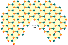
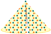
Figure 2: (Color online) Removing a wedge from the graphene (left) and identifying the edges (right), a cone results. The motion of the charge carriers in an ideal conical graphene is equivalent to that of a massless Dirac particle in a gravitational field of a static particle of mass $M$ in a $(2+1)D$ space-time.

To study the scattering of the carriers in graphene by topological defects we employ the analogy between defects in condensed matter physics and in $(2+1)$-dimensional gravity Volovik03 as far as possible. For example, the dynamics of charge carriers in an ideal conical graphene is equivalent to that of a massless Dirac particle in a gravitational field of a static point-like mass in a $(2+1)D$ space-timeFurtado08 ; Brown88 ; Souza89 . Specifically, we shall consider one of the simplest curved manifold, which is associated to the Schwarzschild solution in $(2+1)$ dimensions: a space-time locally flat with global nontrivial properties described below.

To proceed further, we summarize some aspects of general relativity in three space-time dimensions. It fundamentally differs from its 4-dimensional counterpart. Indeed, it exhibits some unusual features, which can be deduced from the properties of the Einstein field equations and the Riemann curvature tensor $R^{\mu}_{\;\;\upsilon\varepsilon\kappa}$ Brown88 ; Staruszkiewikz63 . In regions free of matter (where the momentum-energy tensor $T^{\mu\nu}$ vanishes), the space-time is locally flat when the cosmological constant is zero (the Einstein tensor $G^{\mu\nu}$ vanishes). However, this does not mean that a massive source has no gravitational effects: a light beam passing by a massive, point-like mass will be deflected Staruszkiewikz63 ; Deser84 ; Giddings84 ; Vilenkin81 and parallel transport in a closed circuit around it will in generally gives nontrivial results Burges85 ; Bezerra87 . Indeed, while the local curvature vanishes outside the sources, there are nontrivial global effects. For instance, for the special case of a point-like mass, $M$, sitting at rest in the origin, the line element is given by

$$ds^{2}=dt^{2}-d\rho^{2}-\rho^{2}\alpha^{2}d\theta^{2},$$ (30)

with $0\leq\theta<2\pi$ and $\alpha=1-4GM$ ($G$ is the Newton’s constant, with dimensions of $[length]^{1}$ instead of $[length]^{2}$, in natural units $\hbar=c=1$). Note that although the situation looks trivial, the coordinate $\theta$ ranges from $0$ to $2\pi\alpha$, indicating an angular deficit in space. Then, the spatial part of the metric is that of a plane with a wedge removed and edges identified; the unique $2D$ spatial geometry satisfying this description is the cone Staruszkiewikz63 .

Alternatively, one may use embedded coordinates $r$ and $\theta$ in the three-dimensional Euclidian space which extend over the complete range, $0\leq r\leq\infty\,,\,0\leq\theta\leq 2\pi$, and describe a cone with the constraint $z=\sqrt{(\alpha^{-2}-1)(x^{2}+y^{2})}$, being the line element given by Souza89 :

$$ds^{2}=dt^{2}-\alpha^{-2}dr^{2}-r^{2}d\theta^{2}.$$ (31)

The attributes of the source are coded in the global properties of the locally flat variables. All the information lies in the non-trivial boundary conditions, which is important for the quantum scattering of graphene charge carriers by defects, like pentagons and heptagons.

In the case of a topological defect in graphene, it is useful to change the gravitational term $4GM$ by the symbol $\beta$, so that $2\pi\beta$ (for $0<\beta<1$) gives the deficit of angle measuring the magnitude of the removed sector whereas $-2\pi\beta$ (for $-\infty<\beta<0$) accounts for the angle in excess associated to the insertion of a sector. The parameter $\beta$ takes only discrete values because of the lattice symmetry of the graphene as discussed after eq. (29).

Figure 3: (Color online) Classical trajectories (bue and red) of the scattered particles deflecteds by heptagons (above) and pentagons (below). The trajectories are the asymptotic motion on cone projected onto $x-y$ plane of the embedding three dimensional space, see the text.

Before analyzing the quantum mechanical scattering by conical defects (pentagons and heptagons) let us make a digression concerning scattering of the charge carriers in graphene as classical relativistic particles. The classical equation of motion, determined by relativistic geodesic equation for the particles in a cone reads $\ddot{x}+\Gamma^{\mu}_{\alpha\beta}\dot{x}^{\alpha}\dot{x}^{\beta}=0,$ where the overdot indicates differentiation with respect to any convenient affine variable $\tau$ that parametrizes the path $x^{\mu}(\tau)$ Souza89 . The angle of scattering $\pm\omega$ for the motion of the particles in a cone can be obtained by integration of the classical equations of motion and is given by Souza89 .

$$\pm\omega=\pm\pi(\alpha^{-1}-1)=\pm\pi\frac{\beta}{1-\beta},$$ (32)

where $\pm$ refers to the side the charge carriers (current) trajectory pass around the defect, see (Fig. 3). Note that the result above is valid for all values of $\beta$ despite the sector was removed or inserted. The scattering angle above, presented in the embedded coordinate system (31) measures the deflection of the asymptotic motion on cone projected onto $x-y$ plane of the embedding three dimensional space. The result above suggests that a pentagon or heptagon may be used for deviating the planar current in graphene.

To obtain the correct current deviations in graphene we have to solve the Dirac equation (1) defined in a cone, say Souza89 :

$$i\hbar\gamma^{\mu}E_{a}\,^{\mu}D_{\mu}\psi=0\,,$$ (33)

where $D_{\mu}=\partial_{\mu}+\frac{1}{2}\omega_{\mu;ab}\sigma^{ab}$, $\sigma^{ab}=\frac{1}{4}[\gamma^{a},\gamma^{b}]$, and $E_{a}\,^{\mu}$ is the dreibein in coordinates $(t,r,\theta)$. The spin connection $\omega_{\mu;ab}=-\omega_{\mu;ba}$ may be written in three dimensions as $\omega_{\mu;ab}=\epsilon_{abc}\omega_{\mu}\,^{c}$ with $\epsilon_{abc}$ the Levi-Civita symbol as before Souza89 . The rotational invariance of the problem enables us to choose positive energy solutions that are simultaneously angular momentum eigenfunctions, with eigenvalue $(n+\frac{1}{2})\hbar$:

$$u_{n}(r)e^{-iEt/\hbar}=e^{i(n+\frac{1}{2}-\frac{1}{2}\sigma^{3})\theta}\left(\begin{array}[]{c}u_{n}^{A}(r)\\ u_{n}^{B}(r)\\ \end{array}\right)e^{-iEt/\hbar}\,,$$ (34)

where $n=0,\pm 1,\pm 2,\ldots\,.$ The solutions for $E>0$ are Souza89 :

$$u_{n}^{A}(r)=(\epsilon_{n})^{n}J_{\nu}(\kappa r)\,,$$ (35)

$$u_{n}^{B}(r)=(\epsilon_{n})^{n+1}J_{\nu}(\kappa r).$$ (36)

Here, $J_{\nu}$ is the Bessel function of order $\nu\equiv\epsilon_{n}/\alpha(n+(1\mp\alpha)/2)$, $n=0,\,\pm 1,\,\pm 2\,,\ldots,$ $\kappa=E/\hbar v_{F}\alpha\,,E>0\,,\epsilon_{n}=\pm 1$ and the same sign has to be chosen for the upper and lower components of the spinor $u_{n}(r)$. For $0<\alpha\leq 1$ or $0<\beta\leq 1$ (remember that $\alpha=1-\beta$) we must choose $\epsilon_{n}={\rm sign}(n+(1-\alpha)/2)={\rm sign}\,n\,({\rm sign}\,0\equiv\,1)$ to have both components regular at the origin. The asymptotic form of the Bessel functions determines the phase shifts (they are identical for the upper and lower components)and are given by Souza89 :

$$\delta_{n} = -\epsilon_{n}\frac{\pi}{2\alpha}((1-\alpha)n+(1-\alpha)/2)$$ (37)

$$= -\frac{\epsilon_{n}}{2}\pi\frac{\beta}{1-\beta}\Big{(}n-\frac{1}{2}\Big{)}\,,$$

$$\epsilon_{n}={\rm sign}(n+(1-\alpha)/2)={\rm sign}(n+\beta/2)\,.$$ (38)

The phase-shifts depend only on the number of sectors removed or inserted in the graphene sheet, accounted by $\alpha=1-\beta$. If $-\infty<\beta<0$, we need to be careful because $\epsilon_{n}=\pm 1$ depending upon the value of $(n+\beta/2)$ (but the phase-shifts remains as above) and the phase-shifts depends only on the number of sectors (heptagons) inserted in the flat graphene sheet. In the presence of heptagons the carriers dynamics is identical to the that movement of the electrons in the gravitational field of a negative mass (although not possible in gravitation, this is feasible in the present context).

Note that the phase shift (37) measures the deflection of the asymptotic motion on the cone projected onto $x-y$ plane being qualitatively identical to the classical case discussed before. When there is a pentagon into the lattice and the fermionic current is constrained to pass around and sufficiently close to it such a current is scattered by the defect with an angle which depends only on the number of sectors removed in the graphene and on the side current passed (see Fig. 3). After passing by the pentagon the scattered current trajectories cross and yields an interference pattern. In the case of a heptagon, such a current is scattered but the trajectories diverge each other.

The presence of pentagons or heptagons in the sheet of graphene may manifest as fluctuations in the concentration of charge carriers, modifying several physical properties. For instance, in a planar graphene, it is known that the hopping of electrons between sublattices produces an effective magnetic field which is proportional, in magnitude and direction, to the momentum measured from the Brillouin-zone corners. This effective field, which acts on the pseudospin, may suffer important changes in the conical graphene because a hopping of a quasiparticle, which was previously, say, in the $A$ sublattice, will make it to become out of phase with all quasiparticles occupying the $B$ sublattice.

IV Conclusions

We have studied the scattering of graphene quasiparticles by topological defects like holes, pentagons and heptagons. We obtain the phase shift of the wave-function in all cases. For the case of holes, the main contribution concerns the $s$ scattering and even in this case they do not change the resistivity of the sample, at least at low concentrations (like occurs to short range potential impurities).

We realize that when the fermionic current is constrained to move near and around of pentagons and heptagons introduced in the lattice, it is scattered with an angle that depends only on the number of defects and on which side the current taken. Such a deviation may be determined by means of a Young-type experiment, through the interference pattern between the two currents scattered by the pentagon. In the case of a heptagon such a current is also scattered but it diverges from the defect. Perhaps these effects could be used to build channels of currents in future electronic devices using graphene. In addition, graphene would provide an appealing way to experimentally explore general relativity in two spatial dimensions since such effects are predicted by this theory Furtado08 ; Souza89 ; Burges85 ; Bezerra87 .

Conical spaces generated by topological defects like vortices have been recently considered and the quantum mechanical scattering of a nonrelativistic particlehave been considered in the work of Ref. sitenko with results qualitatively similar to those obtained here.

V Acknowledgments

The authors are grateful to C. furtado for having drawn their attention to important references and for discussion. They also thank CNPq, FAPEMIG and CAPES (Brazilian agencies) for financial support.

References

- (1) K.S. Novoselov, A.K. Geim, S.V. Morosov, D. Jiang, Y. Zhang, S.V. Dubonos, I.V. Grigorieva, and A.A. Firsov, Science 306, 666 (2004).
- (2) K.S. Novoselov, A.K. Geim, S.V. Morozov, D. Jiang, M.I. Katsnelson, I.V. Grigorieva, S.V. Dubonos, and A.A. Firsov, Nature 438, 197 (2005).
- (3) A.K. Geim and K.S. Novoselov, Nature Mat.6, 183 (2007).
- (4) A. Catro-Neto, F. Guinea, and N.M. Peres, Phys. World 19, 33 (2006).
- (5) A.K. Geim and P. Kim, Scient. Amer. (April) 90 (2008).
- (6) M.I. Katsnelson, K.S. Novoselov, and K. Geim, Nature Phys. 2, 620 (2006).
- (7) P.R. Wallace, Phys. Rev. 71, 622 (1947).
- (8) M.I. Katsnelson and K.S. Novoselov, Sol. Stat. Comm. 143, 3 (2007).
- (9) A. V. Shytov, M.I. Katsnelson, and L.S. Levitov, Phys. Rev. Lett. 99,236801 (2007).
- (10) A. V. Shytov, M.I. Katsnelson, and L.S. Levitov, Phys. Rev. Lett. 99,246802 (2007).
- (11) M.I. Katsnelson and A.K. Geim, Phil. Trans. R. Soc. A 366, 195 (2008).
- (12) P.M. Morse and H. Feshback, Methods of Theoretical Physics, McGraw-Hill New York (1953).
- (13) G.M. Rutter, J.N. Crain, N.P. Guisinger, T. Li, P.N. First and J.A. Stroscio, Science 313, 219 (2007).
- (14) M.I. Katsnelson F. Guinea and A.K. Geim, Phys. Rev. B 79, 195426 (2009).
- (15) M.I. Katsnelson, Phys. Rev. B 76, 073411 (2007).
- (16) C. Furtado, F. Moraes and A.M. de M. Carvalho, Phys. Lett. A 372, 5368 (2008).
- (17) A. Cortijo and M. A.H. Vozmediano, Nucl. Phys. B 763, 293 (2007).
- (18) Yu.A. Sitenko and M. N.D. Vlasii, Nucl. Phys. B 787, 241 (2007).
- (19) M. Ge, K. Sattler, Chem. Phys. Lett. 220, 192 (1994).
- (20) A. Krishnan, E. Dujardin, M.M.J. Treacy, J. Hugdahl, S. Lynum, and T.W. Ebbesen, Nature 388, 451 (1997).
- (21) G.E. Volovik, The Universe in a Helium Droplet, Clarendon Press, Oxford (2003).
- (22) J.D. Brown, Lower Dimensional Gravity, World Scientific, New Jersey (1988).
- (23) P. de S. Gerbert and R. Jackiw, Commun. Math. Phys. 124, 229 (1989).
- (24) A. Staruszkiewikz, Acta. Phys. Polon. 24, 734 (1963).
- (25) S. Deser, R. Jackiw, and G. ’t Hooft, Ann. Phys. (N.Y.) 152, 220 (1984).
- (26) S. Giddings, J. Abbott, and K. Kuchar, Gen. Relativ. Gravit. 16, 751 (1984).
- (27) A. Vilenkin, Phys. Rev. D 23, 852 (1981).
- (28) C.J.C. Burges, Phys. Rev. D 32, 504 (1984).
- (29) V.B. Bezerra, Phys. Rev. D 35, 2031 (1987).
- (30) Y.A. Sitenko and N. D. Vlasii, quant-ph, arXiv:1002.1250v1 (2010).