Boundary quasi-orthogonality and sharp inclusion bounds for large Dirichlet eigenvalues

Abstract

We study eigenfunctions $\phi_{j}$ and eigenvalues $E_{j}$ of the Dirichlet Laplacian on a bounded domain $\Omega\subset\mathbb{R}^{n}$ with piecewise smooth boundary. We bound the distance between an arbitrary parameter $E>0$ and the spectrum $\{E_{j}\}$ in terms of the boundary $L^{2}$-norm of a normalized trial solution $u$ of the Helmholtz equation $(\Delta+E)u=0$. We also bound the $L^{2}$-norm of the error of this trial solution from an eigenfunction. Both of these results are sharp up to constants, hold for all $E$ greater than a small constant, and improve upon the best-known bounds of Moler–Payne by a factor of the wavenumber $\sqrt{E}$. One application is to the solution of eigenvalue problems at high frequency, via, for example, the method of particular solutions. In the case of planar, strictly star-shaped domains we give an inclusion bound where the constant is also sharp. We give explicit constants in the theorems, and show a numerical example where an eigenvalue around the 2500th is computed to 14 digits of relative accuracy. The proof makes use of a new quasi-orthogonality property of the boundary normal derivatives of the eigenmodes (Theorem 3 below), of interest in its own right. Namely, the operator norm of the sum of rank 1 operators $\partial_{n}\phi_{j}\langle\partial_{n}\phi_{j},\cdot\rangle$ over all $E_{j}$ in a spectral window of width $\sqrt{E}$ — a sum with about $E^{(n-1)/2}$ terms — is at most a constant factor (independent of $E$) larger than the operator norm of any one individual term.

1 Introduction and main results

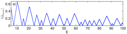
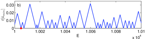
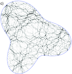
Fig. 1: Tension $t[\tilde{u}_{\mbox{\rm\tiny min}}]$ versus energy $E$ for the domain shown on the right. $\tilde{u}_{\mbox{\rm\tiny min}}$ is the optimal trial Helmholtz solution lying in the span of a numerical basis set (see Section 7). a) Low frequency, showing the minima corresponding to the lowest 20 Dirichlet eigenvalues. b) Medium-high frequency, showing a similar interval starting at eigenvalue number $j\approx 2552$; note the new vertical scale. c) Density plot of eigenfunction $\phi_{j}\approx\tilde{u}_{\mbox{\rm\tiny min}}$ corresponding to the eigenvalue $E_{j}=10005.02135797\cdots$ shown by the dot in b) (black indicates large values of $|\phi_{j}|^{2}$, white zero).

The computation of eigenvalues and eigenmodes of Euclidean domains is a classical problem (in two dimensions this is the ‘drum problem’, reviewed in [21, 34]) with a wealth of applications to engineering and physics, including acoustic, electromagnetic and optical cavity and resonator design, micro-lasers [35], and data analysis [30]. It also has continued interest in mathematical community in the areas of quantum chaos [37, 3] and spectral geometry [18]. Let $\phi_{j}$ be a sequence of orthonormal eigenfunctions and $E_{j}$ the respective eigenvalues ($0<E_{1}<E_{2}\leq E_{3}\leq\cdots$ counting multiplicities) of $-\Delta$, where $\Delta:=\sum_{m=1}^{n}\partial^{2}/\partial x_{m}^{2}$ is the Laplacian in a bounded domain $\Omega\in\mathbb{R}^{n}$, $n\geq 2$, with Dirichlet boundary condition. That is, $\phi_{j}$ satisfies

$$(\Delta+E_{j})\phi_{j} = 0\qquad\mbox{in }\Omega$$ (1)

$$\phi_{j} = 0\qquad\mbox{on }{\partial\Omega}$$ (2)

$$\|\phi_{j}\|_{L^{2}(\Omega)} = 1.$$ (3)

We will call the spectrum $\sigma:=\{E_{j}\}_{j=1}^{\infty}$. Many of the applications mentioned demand high frequencies, that is, mode numbers $j$ from $10^{2}$ to as high as $10^{6}$. Efficient solution of the problem thus requires specialized numerical approaches that scale with wavenumber better than conventional discretization methods.

The goal of this paper is to bound the errors of approximate eigenvalues and eigenfunctions computed using trial functions that satisfy exactly the homogeneous Helmholtz equation in $\Omega$. As we will review below, such computational methods have proven very powerful. Recently one of the authors [4] improved upon the classical eigenvalue bound of Moler–Payne [24] by a factor of the wavenumber; however, this result has limited utility since it applies only to Helmholtz parameters lying in neighborhoods of $\sigma$ of unknown size. In the present paper we go well beyond this result by giving new theorems, which i) hold for all Helmholtz parameters (greater than an $O(1)$ constant), ii) retain the improved high-frequency asymptotic behavior of [4] and show that this behavior is sharp, and iii) improve upon the best-known eigenfunction estimates, again by a factor of the wavenumber. To achieve this we make use of a new form of quasi-orthogonality of the eigenfunctions on the boundary, Theorem 3, of independent interest.

Before presenting our results, we need to review some known inclusion bounds and their importance for applications. Given an energy parameter $E>0$, let $u$ be a non-trivial solution to the homogeneous Helmholtz equation $(\Delta+E)u=0$ in $\Omega$ with no imposed boundary condition, and define its boundary error norm (or ‘tension’)

$$t[u]:=\frac{\|u\|_{L^{2}({\partial\Omega})}}{\|u\|_{L^{2}(\Omega)}}~{}.$$ (4)

Clearly, $t[u]=0$ implies that $E$ is an eigenvalue. It is reasonable to expect that if $t[u]$ is small for some Helmholtz solution $u$, then $E$ is close to an eigenvalue. Moler–Payne [24] (building upon [16]) quantified this: there is a constant $C_{\mbox{\rm\tiny MP}}$ depending only on the domain, such that

$${d(E,\sigma)}\;\leq\;C_{\mbox{\rm\tiny MP}}E\,t[u]~{},$$ (5)

where ${d(E,\sigma)}:=\min_{j}|E_{j}-E|$ denotes the distance of $E$ from the spectrum.

An important application is to solving (1)-(3) via global approximation methods, including the method of particular solutions (MPS) [9, 4]. One writes a trial eigenmode $u=\sum_{n=1}^{N}c_{n}\xi_{n}$ via basis functions $\xi_{n}$ which are closed-form Helmholtz solutions in $\Omega$ but which need not satisfy any particular boundary condition. By adjusting the coefficients $c_{n}$ (via a generalized eigenvalue [4] or singular value problem [8]) one may minimize $t[u]$ at fixed $E$; by repeating this in a search for $E$ values where the minimum $t[u]$ is very small, as illustrated by Fig. 1a and b, one may then locate approximate eigenvalues whose error is bounded above by (5). (This is sometimes called the method of a priori-a posteriori inequalities [21, Sec. 16].)

Due to the work of Betcke–Trefethen [9] and others, such methods have enjoyed a recent revival, at least in $n=2$, due to their high (often spectral) accuracy and their efficiency at high frequency when compared to direct discretization methods such as finite elements. For example, in various domains, 14 digits may be achieved in double precision arithmetic [9], and with an MPS variant known as the scaling method, tens of thousands of eigenmodes as high as $j\sim 10^{6}$ have been computed [3, 5]. (There are also successful variants [14, 15] by Descloux–Tolley, Driscoll, and others, in which subdomains are used, which we will not pursue here.)

If we instead interpret $u$ as the solution error for an interior Helmholtz boundary-value problem (solved, for instance, via MPS or boundary integral methods), then (5) states that the interior error is controlled by the boundary error; this aids the numerical analysis of such problems [22, 6]. Similar estimates (which, however, rely on impedance boundary conditions) enable the analysis of least-squares non-polynomial finite element methods [25, Thm 3.1]. Improving such estimates could thus be of general benefit for the numerical solution of Helmholtz problems.

Recently one of the authors [4] observed numerical evidence that (5) is not sharp for large $E$, and showed that there is a constant $C_{\mbox{\rm\tiny B}}$ depending only on $\Omega$, such that, for each $\varepsilon>0$,

$${d(E,\sigma)}\;\leq\;C_{\mbox{\rm\tiny B}}(1+\varepsilon)\sqrt{E}\,t[u]$$ (6)

holds whenever $E$ lies in some open, possibly disconnected, subset of the real axis containing $\sigma$. This is an improvement over (5) by a factor of the wavenumber $\sqrt{E}$, which in problems of interest can be as high as $10^{3}$. However, since the proof relied on analytic perturbation in the parameter $E$, there was no knowledge about the size of this ($\varepsilon$-dependent) subset, hence no way to know in a given practical situation whether the error bound holds. The point of the present work is then to remedy this problem by removing any restriction to an unknown subset, and also to extend the $\sqrt{E}$ improvement to bounds on approximate eigenfunctions.

We assume the domain $\Omega\subset\mathbb{R}^{n}$ has unit area (or volume for $n>2$), and obeys the following rather weak geometric condition.

Condition 1.

The domain $\Omega\subset\mathbb{R}^{n}$ is bounded, with piecewise smooth boundary in the sense of Zelditch–Zworski [38]. This means that $\Omega$ is given by an intersection

$$\Omega=\bigcap_{i=1}^{N}\{{\mathbf{x}}\mid f_{i}({\mathbf{x}})>0\},$$

where the $f_{i}$ are smooth functions defined on a neighborhood of $\overline{\Omega}$ such that

• $\nabla f_{i}\neq 0$ on the set $\{f_{i}=0\}$,

• $\{f_{i}=f_{j}=0\}$ is an embedded submanifold of $\mathbb{R}^{n}$, $1\leq i<j\leq N$, and

• $\Omega$ is locally Lipschitz, i.e. for any boundary point ${\mathbf{x}}_{0}\in\partial\Omega$, there is a Euclidean coordinate system $z_{1},\dots,z_{n}$ and a Lipschitz function $k$ of $n-1$ variables such that in some neighborhood of ${\mathbf{x}}_{0}$, we have

  $$\partial\Omega=\{z_{n}=k(z_{1},\dots,z_{n-1})\}.$$ (7)

Our main result on eigenvalue inclusion is the following.

Theorem 1.

Let $\Omega\subset\mathbb{R}^{n}$ be a domain satisfying condition 1. Then there are constants $C,c$ depending only on $\Omega$, such that the following holds. Let $E>1$ and suppose $u$ is a non-trivial solution of $(\Delta+E)u=0$ in $C^{\infty}(\Omega)$, with $t[u]:=\|u\|_{L^{2}({\partial\Omega})}/\|u\|_{L^{2}(\Omega)}$. Then,

$${d(E,\sigma)}\;\leq\;C\sqrt{E}\,t[u]~{},$$ (8)

and for the normalized Helmholtz solution $u_{\mbox{\rm\tiny min}}$ minimizing $t[u]$ at the given $E$,

$$c\sqrt{E}\,t[u_{\mbox{\rm\tiny min}}]\;\leq\;{d(E,\sigma)}\;\leq\;C\sqrt{E}t[u_{\mbox{\rm\tiny min}}].$$ (9)

Remark 1.1.

The estimate (9) states that (8) is sharp, i.e., using $t[u]$ alone one cannot localize the spectrum any more tightly than this, apart from optimizing the constants $c$ and $C$.

Remark 1.2.

The existence of a minimizer for $t[u]$ follows from Lemma 7, in the case that $E$ is not a Dirichlet eigenvalue (and is trivial when $E$ is a Dirichlet eigenvalue). The lower bound on the distance to the spectrum in (9) is of use when the numerical scheme is known to produce a good approximation to $u_{\mbox{\rm\tiny min}}$.

We will also prove the following corresponding bound on the error of the trial eigenfunction $u$, which improves by a factor $\sqrt{E}$ the previous best known result (Moler–Payne [24, Thm. 2]).

Theorem 2.

Let $\Omega$ be as in Theorem 9. Then there is a constant $C$ depending only on $\Omega$, such that the following holds. Let $E>1$, let $E_{j}$ be the eigenvalue nearest to $E$, and let $E_{k}$ the next nearest distinct eigenvalue. Suppose $u$ is a solution of $(\Delta+E)u=0$ in $C^{\infty}(\Omega)$ with $\|u\|_{L^{2}(\Omega)}=1$, and let $\hat{u}_{j}$ be the projection of $u$ onto the $E_{j}$ eigenspace. Then,

$$\|u-\hat{u}_{j}\|_{L^{2}(\Omega)}\;\leq\;C\frac{\sqrt{E}\,t[u]}{|E-E_{k}|}~{}.$$ (10)

Remark 1.3.

The left-hand side above is equal to $\sin\theta$, where $\theta$ is the subspace angle between $u$ and the $E_{j}$ eigenspace (this viewpoint is elaborated in [9, Sec. 6]). For example, when $E_{j}$ is a simple eigenvalue, we may write $\|u-\phi_{j}\|_{L^{2}(\Omega)}=2\sin(\theta/2)$.

Remark 1.4.

This result is also sharp, in a certain sense: see Remark 4.1.

To conclude the introduction, we present some key ingredients of the proofs. Define the boundary functions of the eigenmodes by

$$\psi_{j}(s):=\partial_{n}\phi_{j}(s)\qquad s\in{\partial\Omega}$$ (11)

where $\partial_{n}={\mathbf{n}}\cdot\nabla$ is the usual normal derivative. Our main tools will be two theorems stating that boundary functions $\psi_{j}$ lying close in eigenvalue are almost orthogonal. The first is the following new result which we prove in Section 2.

Theorem 3 (spectral window quasi-orthogonality).

Let $\Omega\subset\mathbb{R}^{n}$ be a domain satisfying Condition 1. There exists a constant $C_{\Omega}$ depending only on $\Omega$ such that the operator norm bound

$$\Bigl{\|}\sum_{|E_{j}-E|\leq E^{1/2}}\!\!\psi_{j}\langle\psi_{j},\cdot\rangle\Bigr{\|}_{L^{2}(\partial\Omega)\to L^{2}(\partial\Omega)}\;\leq\;C_{\Omega}E$$ (12)

holds for all $E\geq 1$. (Here, $\langle\cdot,\cdot\rangle$ denotes the inner product in $L^{2}(\partial\Omega)$.)

Remark 1.5.

By Weyl’s Law [17, Ch. 11] there are $O(E^{(n-1)/2})$ terms in the above sum. Since each term already has norm $\geq cE$ [28, 19], the theorem expresses essentially complete mutual orthogonality, up to a constant. Only the scaling of the window width with $E$ is important: the theorem also holds for a window $|E_{j}-E|\leq cE^{1/2}$ for any fixed $c$ ($C_{\Omega}$ will then depend on $c$ as well as $\Omega$). On the other hand, one could not expect it to hold over a spectral window of width $O(E^{\beta})$ for $\beta>1/2$, since the boundary functions are approximately band-limited to spatial wavenumber $E^{1/2}$ and thus no more than $O(E^{(n-1)/2})$ of them could be orthogonal on the boundary.

The second result is a pairwise estimate on the inner product of boundary functions lying close in eigenvalue, with respect to a special inner product: (Here, ${\mathbf{x}}(s)$ refers to the location of boundary point $s$ relative to a fixed origin, which may or may not be inside $\Omega$.)

Theorem 4 (pairwise quasi-orthogonality).

Let $\Omega\subset\mathbb{R}^{n}$ be a bounded Lipschitz domain, and let $S:=\frac{1}{2}\sup_{{\mathbf{x}}\in\Omega}\|{\mathbf{x}}\|$. Then, for all $i,j\geq 1$,

$$\Big{|}\int_{{\partial\Omega}}({\mathbf{x}}(s)\cdot{\mathbf{n}}(s))\,\psi_{i}(s)\psi_{j}(s)\,ds-2E_{i}\delta_{ij}\Big{|}\;\leq\;S^{2}(E_{i}-E_{j})^{2}$$ (13)

Remark 1.6.

This theorem was proved by the first-named author in [3, Appendix B]. It may be viewed as an off-diagonal generalization of a theorem of Rellich [28] which gives the $i=j$ case. The boundary weight ${\mathbf{x}}\cdot{\mathbf{n}}$ (also known as the Morawetz multiplier) is the only one known that gives quadratic growth away the diagonal yet also gives non-zero diagonal elements.

Note that neither of the above quasi-orthogonality theorems implies the other. We also note that Bäcker et al. derived a completeness property of the boundary functions in a (smoothed) spectral window [2, Eq. (53)], that is closely related to Theorem 3.

After proving Theorem 3, we combine it with a boundary operator defined in Section 3 to prove the main theorems, in Section 4. In Section 5 we state and prove a variant of Theorem 9 for strictly star-shaped planar domains, which has an optimal constant $C$. This builds on Theorem 13 combined with the Cotlar-Stein lemma (see Lemma 11). In the main Theorems 9, 10 and 51, the domain-dependent constants are not explicit; we discuss their explicit values in Section 6. We present a high-accuracy numerical example using the MPS, and sketch some of the implementation aspects, in Section 7. Finally, we conclude in Section 8.

2 Quasi-orthogonality in an eigenvalue window

Here we prove Theorem 3 using a “$TT^{\ast}$ argument”. We need the fact that the upper bound $\|\psi_{j}\|_{L^{2}(\partial\Omega)}^{2}\leq CE_{j}$ on eigenmode normal derivatives, proved for example in [19], generalizes to quasimodes living in an $O(E^{1/2})$ spectral window. The proof is almost the same as in [19].

Lemma 5.

Let $\Omega\subset\mathbb{R}^{n}$ satisfy Condition 1. Let $E>1$, and let

$$\phi:=\sum_{|E_{j}-E|\leq E^{1/2}}\!\!c_{j}\phi_{j}$$ (14)

with real coefficients $c_{j}$, and $\sum_{j}c_{j}^{2}=\|\phi\|^{2}_{L^{2}(\Omega)}=1$. Then,

$$\|\partial_{n}\phi\|^{2}_{L^{2}({\partial\Omega})}\;\leq\;C_{\Omega}E$$ (15)

where the constant $C_{\Omega}$ depends only on $\Omega$.

Proof.

To prove this we need the following lemma, proved in Appendix A, stating that for any piecewise smooth domain (in the sense of Condition 1) there is a smooth vector field that is outgoing at each boundary point.

Lemma 6.

Let $\Omega$ satisfy Condition 1. Then there exists a smooth vector field ${\mathbf{a}}$, defined on a neighborhood of $\overline{\Omega}$, such that

$${\mathbf{a}}\cdot{\mathbf{n}}\geq 1$$ (16)

almost everywhere on $\partial\Omega$.

The main tool for proving Lemma 5 is the identity

$$\int_{\partial\Omega}(D\phi)\partial_{n}\phi=-\int_{\Omega}\phi[\Delta,D]\phi+\int_{\Omega}(D\phi)(\Delta+E)\phi-\int_{\Omega}\phi D(\Delta+E)\phi$$ (17)

for any first order differential operator $D$, which follows from Green’s 2nd identity, the definition of the commutator, and $\phi|_{\partial\Omega}=0$. Choosing $D:={\mathbf{a}}\cdot\nabla$, where ${\mathbf{a}}$ is as in Lemma 6, we notice that the left-hand side of (17) bounds the left-hand side of (15), since

$$\int_{\partial\Omega}\psi_{j}^{2}\;\leq\;\int_{\partial\Omega}({\mathbf{a}}\cdot{\mathbf{n}})\psi_{j}^{2}$$ (18)

by Condition 1. We may now bound each of the terms on the right-hand side of (17). Defining $C_{a}=\sup_{{\mathbf{x}}\in\Omega}|{\mathbf{a}}({\mathbf{x}})|$, we have

$$\|D\phi\|_{L^{2}(\Omega)}^{2}\leq C_{a}^{2}\int_{\Omega}\|\nabla\phi\|^{2}=-C_{a}^{2}\int_{\Omega}\phi\Delta\phi=C_{a}^{2}\sum_{j}|c_{j}|^{2}E_{j}\leq C_{a}^{2}F$$ (19)

where $F:=E+E^{1/2}$ is the upper end of the window. Similarly,

$$\|D(\Delta+E)\phi\|_{L^{2}(\Omega)}^{2} \leq C_{a}^{2}\int_{\Omega}\|\nabla(\Delta+E)\phi\|^{2}=C_{a}^{2}\sum_{ij}c_{i}c_{j}\int_{\Omega}(\Delta+E)\phi_{i}(-\Delta)(\Delta+E)\phi_{j}$$ (20)

$$= C_{a}^{2}\sum_{j}c_{j}^{2}E_{j}(E-E_{j})^{2}\leq C_{a}^{2}EF~{}.$$

Using Cauchy-Schwarz, the sum of the last two terms in (17) is then bounded by $2C_{a}\sqrt{EF}$. For the first term on the right of (17), we use Einstein notation $[\Delta,D]=\partial_{ii}(a_{j}\partial_{j}\cdot)-a_{j}\partial_{iij}$. After several steps, using integration by parts and $\phi|_{\partial\Omega}=0$, we get

$$-\int_{\Omega}\phi[\Delta,D]\phi=2\int_{\Omega}(\partial_{i}a_{j})(\partial_{i}\phi)\partial_{j}\phi+\int_{\Omega}(\partial_{ii}a_{j})\phi\partial_{j}\phi$$ (21)

The constants $C^{\prime}_{a}:=\sup_{{\mathbf{x}}\in\Omega}\|\mathbb{A}({\mathbf{x}})\|_{2}$ where the matrix $\mathbb{A}\in\mathbb{R}^{n\times n}$ has entries $\partial_{i}a_{j}$, and $C^{\prime\prime}_{a}:=\sup_{{\mathbf{x}}\in\Omega,j=1,\ldots,n}|\Delta a_{j}({\mathbf{x}})|$, exist and are finite. Then (21) is bounded by $2C^{\prime}_{a}F+C^{\prime\prime}_{a}F^{1/2}$. Adding all bounds on terms in (17) we get

$$\|\partial_{n}\phi\|^{2}_{L^{2}({\partial\Omega})}\leq 2(C_{a}+C^{\prime}_{a})F+C^{\prime\prime}_{a}\sqrt{F}~{},$$ (22)

which is bounded by a constant times $E$ for $E>1$. ∎

Proof of Theorem 3. Consider the coefficient vector ${\mathbf{c}}:=\{c_{j}\}\in\mathbb{R}^{N}$ appearing in (14), where $N$ is the number of eigenvalues (counting multiplicity) in the spectral window. Define the linear operator $T:\mathbb{R}^{N}\to{L^{2}({\partial\Omega})}$ by

$$T{\mathbf{c}}=\sum_{j}c_{j}\psi_{j}$$ (23)

Lemma 5 states that $\|T\|_{l^{2}\to{L^{2}({\partial\Omega})}}\leq(C_{\Omega}E)^{1/2}$. Thus $\|TT^{\ast}\|_{L^{2}({\partial\Omega})}\leq C_{\Omega}E$. But $TT^{\ast}$ is the operator in the statement of Theorem 3, which completes its proof.

3 Relating tension to a boundary operator

In this section, we show, following Barnett [4], that the tension $t[u]$ is related to the operator norm of a natural boundary operator.

For $E$ a non-eigenvalue of $\Omega$, let ${\cal K}(E):{L^{2}({\partial\Omega})}\to{L^{2}(\Omega)}$ be the solution operator (Poisson kernel) for the interior Dirichlet boundary-value problem,

$$(\Delta+E)u = 0\qquad\mbox{ in }\Omega$$ (24)

$$u = f\qquad\mbox{ on }{\partial\Omega}~{},$$ (25)

that is, $u={\cal K}f$. (For existence and uniqueness for $L^{2}$ data on a Lipschitz boundary see for example [23, Thm. 4.25].) Since the eigenbasis is complete in ${L^{2}(\Omega)}$, we may write $u=\sum_{j=1}^{\infty}c_{j}\phi_{j}$. We evaluate each $c_{j}$ by applying Green’s 2nd identity,

$$(E-E_{j})(\phi_{j},u)_{L^{2}(\Omega)}=\int_{\Omega}(u\Delta\phi_{j}-\phi_{j}\Delta u)=\int_{\partial\Omega}(f\psi_{j}-\phi_{j}\partial_{n}u)ds~{},$$ (26)

thus $c_{j}=\langle\psi_{j},f\rangle/(E-E_{j})$. The solution operator may therefore be written as a sum of rank-1 operators,

$${\cal K}(E)=\sum_{j=1}^{\infty}\frac{\phi_{j}\langle\psi_{j},\cdot\rangle}{E-E_{j}}~{}.$$ (27)

By the definition (4) we have, now for any $u$ satisfying $(\Delta+E)u=0$ in $\Omega$, that $t[u]^{-1}\leq\|{\cal K}(E)\|$. Since $\|{\cal K}^{\ast}{\cal K}\|=\|{\cal K}\|^{2}$, then by defining the boundary operator in ${L^{2}({\partial\Omega})}\to{L^{2}({\partial\Omega})}$,

$$A(E):={\cal K}(E)^{\ast}{\cal K}(E)~{},$$ (28)

we have an estimate on the tension that will be the main tool in our analysis,

$$t[u]^{-2}\;\leq\;\|A(E)\|~{}.$$ (29)

Inserting (27) into (28) and using orthogonality (or see [4, Sec. 3.1]), we have that $A$ also may be written as the sum of rank-1 operators,

$$A(E)=\sum_{j=1}^{\infty}\frac{\psi_{j}\langle\psi_{j},\cdot\rangle}{(E-E_{j})^{2}}$$ (30)

This sum is conditionally convergent: the sum of the operator norm of each term diverges. For instance, for $n=2$, Weyl’s law [17, Ch. 11] states that the density of eigenvalues $E_{j}$ is asymptotically constant, but since $\|\psi_{j}\|^{2}=\Omega(E_{j})$ the sum of norms is logarithmically divergent; for $n>2$ the divergence is worse. Despite this, we have the following, which improves upon the results of [4].

Lemma 7.

Let $\Omega\subset\mathbb{R}^{n}$, $n\geq 2$, satisfy Condition 1, and let $E>0$. Then

$$\lim_{N\to\infty}\ \ \sum_{j=1}^{N}\frac{\psi_{j}\langle\psi_{j},\cdot\rangle}{(E-E_{j})^{2}}$$ (31)

converges in the norm operator topology. Furthermore, the limit operator $A(E)$ is compact in ${L^{2}({\partial\Omega})}$.

Proof.

This follows immediately from (39) in the proof of Lemma 38 below, which shows that the tail of the sum in (30) has vanishing operator norm. $A$ is therefore also the norm limit of a sequence of finite-rank operators. ∎

4 Proof of Theorems 9 and 10

In the previous section we related tension to the norm of a boundary operator which itself can be written as a sum involving mode boundary functions. Here we place upper bounds on $\|A(E)\|$ in order to prove Theorems 9 and 10. Firstly we note that when $E$ is an eigenvalue, Theorem 9 is trivially satisfied, since $t[u_{\mbox{\rm\tiny min}}]=0$. When $E$ is a non-eigenvalue, formula (30) enables us to split up contributions from different parts of the Dirichlet spectrum,

$$A(E)=A_{\mbox{\rm\tiny near}}(E)+A_{\mbox{\rm\tiny far}}(E)+A_{\mbox{\rm\tiny tail}}(E)$$ (32)

where

$$A_{\mbox{\rm\tiny near}}(E) = \sum_{|E_{j}-E|\leq E^{1/2}}\frac{\psi_{j}\langle\psi_{j},\cdot\rangle}{(E-E_{j})^{2}}$$ (33)

$$A_{\mbox{\rm\tiny far}}(E) = \sum_{E/2\leq E_{j}\leq 2E,\,|E_{j}-E|>E^{1/2}}\frac{\psi_{j}\langle\psi_{j},\cdot\rangle}{(E-E_{j})^{2}}$$ (34)

$$A_{\mbox{\rm\tiny tail}}(E) = \sum_{E_{j}<E/2}\frac{\psi_{j}\langle\psi_{j},\cdot\rangle}{(E-E_{j})^{2}}+\sum_{E_{j}>2E}\frac{\psi_{j}\langle\psi_{j},\cdot\rangle}{(E-E_{j})^{2}}$$ (35)

It is sufficient (due to the operator triangle inequality) to bound the norms of these three terms independently. We first tackle the “far” and “tail” terms.

Lemma 8.

There is a constant $C$ dependent only on $\Omega$ such that

$$\bigl{\|}A_{\mbox{\rm\tiny far}}(E)\bigr{\|}\;\leq\;C\qquad\mbox{ for all }E>1$$ (36)

Proof.

For any $E>1$, consider the spectral interval $I_{m}:=[E+mE^{1/2},E+(m+1)E^{1/2}]$. For any such interval lying in $[E/2,2E]$ we may apply Theorem 3, with $E$ replaced by at most $2E$, to bound $\|\sum_{E_{j}\in I_{m}}\psi_{j}\langle\psi_{j},\rangle\|$ by $2C_{\Omega}E$. For terms in (34) associated with this interval, the denominators are no less than $m^{2}E$. Thus

$$\Bigl{\|}\sum_{E_{j}\in I_{m}}\frac{\psi_{j}\langle\psi_{j},\cdot\rangle}{(E-E_{j})^{2}}\Bigr{\|}\;\leq\;\frac{2C_{\Omega}}{m^{2}}$$ (37)

Covering $[E+E^{1/2},2E]$ by summing over $m=1,2,\ldots$ gives a constant, since $\sum m^{-2}=\pi^{2}/6$. The same argument applies for intervals covering $[E/2,E-E^{1/2}]$. ∎

Lemma 9.

There is a constant $C$ dependent only on $\Omega$ such that

$$\bigl{\|}A_{\mbox{\rm\tiny tail}}(E)\bigr{\|}\;\leq\;CE^{-1/2}\qquad\mbox{ for all }E>1$$ (38)

Proof.

Consider a spectral interval $I_{m}:=[2^{m}E,2^{m+1}E]$. We may cover this with at most $2^{m/2-1}E^{1/2}+1$ windows of half-width at most $2^{m/2}E^{1/2}$; for each of these windows Theorem 3 applies to bound $\|\sum_{E_{j}\in I_{m}}\psi_{j}\langle\psi_{j},\rangle\|$ by $C_{\Omega}2^{m+1}E$. For each $E_{j}\in I_{m}$, the denominator is no smaller than $(2^{m-1}E)^{2}$. Thus

$$\Bigl{\|}\sum_{E_{j}\in I_{m}}\frac{\psi_{j}\langle\psi_{j},\cdot\rangle}{(E-E_{j})^{2}}\Bigr{\|}\;\leq\;(2^{m/2-1}E^{1/2}+1)\frac{C_{\Omega}2^{m+1}E}{(2^{m-1}E)^{2}}=C_{\Omega}(2^{-m/2-2}E^{-1/2}+2^{-m+1}E^{-1})$$ (39)

The infinite sum over $m=1,2,\ldots$ gives

$$\Bigl{\|}\sum_{E_{j}>2E}\frac{\psi_{j}\langle\psi_{j},\cdot\rangle}{(E-E_{j})^{2}}\Bigr{\|}\leq C_{\Omega}\left(\frac{E^{-1/2}}{4(\sqrt{2}-1)}+2E^{-1}\right)\leq CE^{-1/2}\;\mbox{ for all }E>1.$$ (40)

We treat the interval $(0,E/2)$ similarly, using a sequence of intervals $J_{m}:=[2^{-m-1}E,2^{-m}E]$. Each such interval may be covered by at most $2^{-(m+3)/2}E^{1/2}+1$ windows of half-width $2^{-(m+1)/2}E^{1/2}$. For each $E_{j}\in J_{m}$, the denominator is no smaller than $E^{2}/4$. In a similar manner as before, the operator norm of the partial sum associated with $J_{m}$ is then $O(2^{-m}E^{-1/2})$, thus the infinite sum over $m$ is $O(E^{-1/2})$. Note that Theorem 3 does not apply for $E<1$, but that there are $O(1)$ such $E_{j}$ values and each contributes $O(E^{-1})$. This proves the Lemma. ∎

Proof of Theorem 9. Examining the “near” term (33), we use Theorem 3 on the sum of numerators, and get a bound by taking the minimum denominator,

$$\bigl{\|}A_{\mbox{\rm\tiny near}}(E)\bigr{\|}\;\leq\;\frac{C_{\Omega}E}{{d(E,\sigma)}^{2}}\qquad\mbox{ for all }E>1$$ (41)

Using this and the above Lemmas to sum the terms in (32) gives

$$\bigl{\|}A(E)\bigr{\|}\;\leq\;\frac{C_{\Omega}E}{{d(E,\sigma)}^{2}}+C\qquad\mbox{ for all }E>1$$ (42)

From Lemma 13, an upper bound on the distance to the spectrum, we see that the second term is bounded by at most a constant times the first, so may be absorbed into it to give

$$\bigl{\|}A(E)\bigr{\|}\;\leq\;\frac{CE}{{d(E,\sigma)}^{2}}\qquad\mbox{ for all }E>1$$ (43)

Combining this with (29) proves (8), hence also the second inequality in (9). The first inequality in (9) simply follows from the fact that, since $A$ is a sum of positive operators,

$$t[u_{\mbox{\rm\tiny min}}]^{-2}=\bigl{\|}A(E)\bigr{\|}\geq\Bigl{\|}\frac{\psi_{j}\langle\psi_{j},\cdot\rangle}{(E-E_{j})^{2}}\Bigr{\|}=\frac{\|\psi_{j}\|^{2}}{{d(E,\sigma)}^{2}}~{},$$ (44)

where $E_{j}$ is the eigenvalue closest to $E$. Using the lower bound $\|\psi_{j}\|^{2}\geq cE_{j}$ from [19] this becomes

$${d(E,\sigma)}\geq c\sqrt{E_{j}}t[u_{\mbox{\rm\tiny min}}]~{}.$$ (45)

With a change of constant, $E_{j}$ may be replaced here by $E$ to give the first inequality in (9), since Lemma 13 insures that $E_{j}$ is relatively close to $E$. (The lemma is not useful for $E$ less than some constant and $E_{j}<E$, but then the ratio $E/E_{j}$ is still bounded by a constant because $E_{j}\geq E_{1}$).

Proof of Theorem 10. We next prove the eigenfunction error bound (10), first considering $E$ a non-eigenvalue. We denote the boundary data by $U:=u|_{\partial\Omega}$. From orthogonality, then using the formula for the $c_{i}$ coefficients below (26), we get,

$$\|u-\hat{u}_{j}\|^{2}_{L^{2}(\Omega)}=\sum_{E_{i}\neq E_{j}}|(\phi_{i},u)_{L^{2}(\Omega)}|^{2}=\sum_{E_{i}\neq E_{j}}\frac{|\langle\psi_{i},U\rangle|^{2}}{(E-E_{i})^{2}}\leq\Bigl{\|}\sum_{E_{i}\neq E_{j}}\frac{\psi_{i}\langle\psi_{i},\cdot\rangle}{(E-E_{i})^{2}}\Bigr{\|}\|U\|_{2}^{2}.$$ (46)

The operator in the last expression is identical to (30) except with the $E_{j}$-eigenspace terms omitted. Therefore, its norm may be bounded in the same way as that of $A(E)$, the only difference being that the ${d(E,\sigma)}$ introduced in (41) is replaced by $\min_{E_{i}\neq E_{j}}|E-E_{i}|=|E-E_{k}|$. Thus the bound analogous to (43) is

$$\bigl{\|}\sum_{E_{i}\neq E_{j}}\frac{\psi_{j}\langle\psi_{j},\cdot\rangle}{(E-E_{j})^{2}}\bigr{\|}\;\leq\;\frac{CE}{(E-E_{k})^{2}}\qquad\mbox{ for all }E>1~{},$$

and inserting this and $\|U\|_{L^{2}({\partial\Omega})}=t[u]\|u\|_{L^{2}(\Omega)}=t[u]$ into (46) gives (10). Finally, if $E$ is an eigenvalue, i.e. $E=E_{j}$, the solution operator (27) is undefined, since a solution to (24)-(25) exists if and only if $f$ is orthogonal to the normal derivative functions in the $E$-eigenspace. This can be seen by applying Green’s 2nd identity to $\phi$, any function in the $E$-eigenspace, and $u$, giving $\langle\partial_{n}\phi,U\rangle=0$. However, the solution coefficients $c_{i}$ for which $E_{i}\neq E$ are uniquely defined by the same formula as before. Thus (46) and the rest of the proof carries through.

Remark 4.1.

Theorem 10 is sharp, as can be seen in the following way: if $u$ is such that $t[u]$ is close to $t[u_{{\mbox{\rm\tiny min}}}]$ (say, less than $2t[u_{{\mbox{\rm\tiny min}}}]$), then we have, by combining (9) and (10),

$$\|u-\hat{u}_{j}\|_{L^{2}(\Omega)}\;\leq\;C\frac{|E-E_{j}|}{|E-E_{k}|}~{}.$$ (47)

Apart from the value of the constant, one cannot expect to do better than this. For example, if $E$ is midway between $E_{j}$ and $E_{k}$, then the error $\|u-\hat{u}_{j}\|_{L^{2}(\Omega)}$ cannot be expected to be better than $1/\sqrt{2}$.

5 Star-shaped planar domains

The purpose of this section is to say something stronger than Theorem 9 in the special case of star-shaped domains in $n=2$. We take weighted boundary functions

$$\psi^{(s)}_{j}(s):=({\mathbf{x}}(s)\cdot{\mathbf{n}}(s))\partial_{n}\phi_{j}(s)~{},\qquad s\in{\partial\Omega}$$ (48)

and our boundary inner product as

$$\langle f,g\rangle_{s}:=\int_{\partial\Omega}({\mathbf{x}}(s)\cdot{\mathbf{n}}(s))^{-1}f(s)g(s)ds$$ (49)

hence norm $\|f\|_{s}:=\sqrt{\langle f,f\rangle}$, and $t_{s}[u]:=\|U\|_{s}/\|u\|_{L^{2}(\Omega)}$. The significance of the weight $({\mathbf{x}}\cdot{\mathbf{n}})$ is twofold: it is strictly positive for strictly star-shaped domains, and also turns the inner product in (13) into $\langle\psi^{(s)}_{i},\psi^{(s)}_{j}\rangle_{s}$, enabling us to benefit from pairwise quasi-orthogonality. The Rellich theorem $\|\psi^{(s)}_{j}\|_{s}^{2}=2E_{j}$ states that, with this special weight, there is no fluctuation in the $L^{2}$-norms of the boundary functions. As shown in [4], the function $t_{s}[u_{\mbox{\rm\tiny min}}]$ vs $E$ has slope $1/\|\psi^{(s)}_{j}\|_{s}^{2}$ in the neighborhood of $E_{j}$ (this arises from dominance of a single term in (52) below). Hence these slopes are predictable independently of the particular form of each mode $\phi_{j}$. This enables us to get the following eigenvalue inclusion result analogous to Theorem 9.

Theorem 10.

Let $\Omega\subset\mathbb{R}^{2}$ be a strictly star-shaped bounded domain with piecewise smooth boundary. Then there are constants $c_{1}$, $c_{2}$, $c_{3}$ depending only on $\Omega$, such that the following holds. Let $E>1$, and suppose $u$ is a non-trivial solution of $(\Delta+E)u=0$ in $C^{\infty}(\Omega)$, with $c_{2}t_{s}[u]^{2}<1$. Let $F:=E+\sqrt{E}$. Then,

$${d(E,\sigma)}\;\leq\;\sqrt{2F}\,t_{s}[u]\frac{1+c_{1}\sqrt{F}t_{s}[u]}{1-c_{2}t_{s}[u]^{2}}~{}.$$ (50)

For the Helmholtz solution $u_{\mbox{\rm\tiny min}}$ minimizing $t_{s}[u]$ at the given $E$,

$$\sqrt{2(E-c_{3}E^{1/2})}\,t_{s}[u_{\mbox{\rm\tiny min}}]\;\leq\;{d(E,\sigma)}$$ (51)

Remark 5.1.

In the limit of high frequency $E\gg 1$ and small tension $t_{s}[u]\ll E^{-1/2}$, the right-hand side of (50) and the left hand side of (51) are both $\sqrt{2E}(1+o(1))t_{s}$. This proves that both the power of $E$ and the constant $\sqrt{2}$ are sharp.

Remark 5.2.

Notice that this theorem is not applicable for all $E$ since there may be large spectral gaps where $c_{2}t_{s}[u]^{2}<1$ cannot be satisfied. Due to the numerator, it becomes far from optimal when $t_{s}[u]$ is $O(E^{-1/2})$ or larger. In these respects it is less general than Theorem 9, even though it gives better bounds in the small tension limit.

The main tool used in the proof of Theorem 51 is the pairwise quasi-orthogonality result, Theorem 13, together with the Cotlar-Stein lemma, which we state here for the special case of self-adjoint operators:

Lemma 11 (Cotlar-Stein [12, 32, 11]).

Let $\{T_{j}\}_{j\in J}$ be a countable set of bounded self-adjoint operators, $J\subset\mathbb{N}$. Then

$$\Bigl{\|}\sum_{j\in J}T_{j}\Bigr{\|}\leq\max_{j\in J}\sum_{i\in J}\sqrt{\|T_{i}T_{j}\|}~{}.$$

Proof of Theorem 51. The weighted equivalent of (30) is the operator

$$A^{(s)}(E)=\sum_{j=1}^{\infty}\frac{\psi^{(s)}_{j}\langle\psi^{(s)}_{j},\cdot\rangle_{s}}{(E-E_{j})^{2}}$$ (52)

which, by analogy with (29), satisfies

$$t_{s}[u]^{-2}\;\leq\;\|A^{(s)}(E)\|_{s}~{}.$$ (53)

The lower bound (51) follows by analogy with (44)-(45), using $\|\psi^{(s)}_{j}\|_{s}^{2}=2E_{j}$, and $E_{j}\geq E-c_{3}E^{1/2}$ from Lemma 13.

Using the same splitting into “near”, “far”, and “tail” parts as in Section 4, we can bound the norm of the “near” part in a new way, as follows.

Lemma 12.

There is a constant $c_{1}>0$ depending only on $\Omega$ such that

$$\|A^{(s)}_{\mbox{\rm\tiny near}}(E)\|_{s}\leq\frac{2F}{{d(E,\sigma)}^{2}}+\frac{\sqrt{2}c_{1}F}{{d(E,\sigma)}}\qquad\mbox{ for all }E>1$$

The first term in this bound will arise simply from the single term in the sum (52) with $E_{j}$ nearest to $E$. The second term requires more work, as we now show.

Proof.

Let $J=\{j:|E_{j}-E|\leq E^{1/2}\}$. Using $T_{j}=\frac{\psi_{j}\langle\psi_{j},\cdot\rangle}{(E-E_{j})^{2}}$ in Lemma 11 gives

$$\Bigl{\|}\sum_{j\in J}T_{j}\Bigr{\|}_{s}\;\leq\;\max_{j\in J}\frac{\|\psi^{(s)}_{j}\|_{s}^{1/2}}{|E-E_{j}|}\sum_{i\in J}\frac{\bigl{(}\langle\psi^{(s)}_{i},\psi^{(s)}_{j}\rangle_{s}\,\|\psi^{(s)}_{i}\|_{s}\bigr{)}^{1/2}}{|E-E_{i}|}$$ (54)

Applying quasi-orthogonality (Theorem 13) for the inner product, and $\|\psi^{(s)}_{j}\|_{s}^{2}=2E_{j}$, and separating diagonal ($i=j$) from off-diagonal terms, we get,

$$\Bigl{\|}\sum_{j\in J}\frac{\psi_{j}\langle\psi_{j},\cdot\rangle}{(E-E_{j})^{2}}\Bigr{\|}\;\leq\;\max_{j\in J}\frac{2E_{j}}{(E-E_{j})^{2}}+\sqrt{2}S\max_{j\in J}\frac{E_{j}^{1/4}}{|E-E_{j}|}\sum_{i\in J}\frac{E_{i}^{1/4}|E_{i}-E_{j}|}{|E-E_{i}|}$$ (55)

Here $S$ is as in Theorem 13. The first term is bounded by $2F/{d(E,\sigma)}^{2}$. Using $|E_{i}-E_{j}|\leq|E_{i}-E|+|E-E_{j}|$ bounds the second term by

$$\sqrt{2}S\max_{j\in J}\frac{E_{j}^{1/4}}{|E-E_{j}|}\sum_{i\in J}E_{i}^{1/4}\left(1+\frac{|E-E_{j}|}{|E-E_{i}|}\right)$$ (56)

$$\leq \sqrt{2F}S\,|J|\,\max_{j\in J}\Bigl{(}\frac{1}{|E-E_{j}|}+\frac{1}{{d(E,\sigma)}}\Bigr{)}\;\leq\;\frac{2\sqrt{2F}S|J|}{{d(E,\sigma)}}$$

Recall Weyl’s law for the asymptotic density of eigenvalues, which states that, for $n=2$ and $\operatorname{vol}\Omega=1$,

$$N(E):=\#\{j:E_{j}<E\}=\frac{1}{4\pi}E+R(E)~{},$$ (57)

where the remainder is $R(E)=O(\sqrt{E})$ ([29]; for the case of piecewise-smooth boundary see [31, Eq. (0.3)]). Since the remainder is bounded for small $E$, there is a constant $C_{\mbox{\rm\tiny W}}$ such that $|R(E)|\leq C_{\mbox{\rm\tiny W}}\sqrt{E}$ for all $E>1$. Thus $|J|$, the number of terms in the “near” window, is bounded by

$$|J|\leq\Bigl{(}\frac{1}{4\pi}+2C_{\mbox{\rm\tiny W}}\Bigr{)}\sqrt{F}~{}.$$

Inserting this into (56) proves the Lemma, and we may take $c_{1}=2S(1/4\pi+2C_{\mbox{\rm\tiny W}})$. ∎

Completion of the proof of Theorem 51. The proofs of analogously weighted versions of Lemmas 36 and 38 are unchanged. So we may combine them with Lemma 12 and (53) to get, for some constant $c_{2}$,

$$t_{s}[u]^{-2}\;\leq\;\|A^{(s)}(E)\|_{s}\;\leq\;\frac{2F}{{d(E,\sigma)}^{2}}+\frac{\sqrt{2}c_{1}F}{{d(E,\sigma)}}+c_{2}\qquad\mbox{ for all }E>1$$

Multiplying through by ${d(E,\sigma)}^{2}$ we solve the quadratic inequality for ${d(E,\sigma)}$,

$${d(E,\sigma)}\;\leq\;\frac{c_{1}F/\sqrt{2}+\sqrt{c_{1}^{2}F^{2}/2+2(t_{s}[u]^{-2}-c_{2})F}}{t_{s}[u]^{-2}-c_{2}}$$

Using the subadditivity of the square-root completes the proof of (50).

6 Discussion of explicit constants

For the practical application of Theorems 9 and 10, it is important to have an explicit value for the constant $C$ (from the discussion after (46) we notice that $C$ in the two theorems is the same.)

We now compute an explicit value of this $C$ that holds for all $E>1$. Examining (22) we see that a choice of constant in Lemma 5, and hence Theorem 3, that holds for all $E>1$ is $C_{\Omega}=4(C_{a}+C^{\prime}_{a})+\sqrt{2}C^{\prime\prime}_{a}$. To compute this we need sup norms of the value, and first and second derivative, of a vector field ${\mathbf{a}}$ as in Lemma 6.

The proof of Lemma 6 shows such a construction; the values will depend on the size of the vectors ${\mathbf{a}}_{x_{i}}$ and the choice of partition of unity used to cover $\overline{\Omega}$. The vectors ${\mathbf{a}}_{x_{i}}$ will be large (order $1/\epsilon$) if $\Omega$ has corners with angles less than $\epsilon$ or greater than $2\pi-\epsilon$. We note that a numerical procedure for this construction could be useful.

In some special cases, a simpler prescription for the vector field can be given:

• For strictly star-shaped domains in $\mathbb{R}^{n}$, we may choose ${\mathbf{a}}={\mathbf{x}}/\inf_{\partial\Omega}({\mathbf{x}}\cdot{\mathbf{n}})$, which gives $C_{a}=\sup_{\partial\Omega}({\mathbf{x}}\cdot{\mathbf{n}})/\inf_{\partial\Omega}({\mathbf{x}}\cdot{\mathbf{n}})$, $C^{\prime}_{a}=1/\inf_{\partial\Omega}({\mathbf{x}}\cdot{\mathbf{n}})$, and $C^{\prime\prime}_{a}=0$.

• For a domain with $C^{2}$ boundary, let $\delta>0$ be the largest number such that for each ${\mathbf{x}}_{0}\in\partial\Omega$, a ball of radius $\delta$ can be placed within $\Omega$ so as to be tangent to $\partial\Omega$ at ${\mathbf{x}}_{0}$. We may then choose ${\mathbf{a}}=(1-r/\delta)^{2}{\mathbf{n}}_{r}$, for $r<\delta$, ${\mathbf{a}}={\mathbf{0}}$ otherwise, where the coordinate $r$ is the distance from ${\partial\Omega}$, and ${\mathbf{n}}_{r}$ is the unit vector in the local decreasing $r$ direction. This gives constants $C_{a}=1$ and $C^{\prime}_{a}=2/\delta$. $C^{\prime\prime}_{a}$ depends on $\delta$ and an upper bound on the rate of change of surface curvature. (Also note that a slight modification of the proof of Theorem 3 would allow estimation purely in terms of $C_{a}$ and $C^{\prime}_{a}$, but with a doubling of the numerical constants).

Summing the terms (37) above and below $E$ we have that the constant in Lemma 36 is $2\pi^{2}C_{\Omega}/3$. Similarly, using (40) and its equivalent for $(0,E/2)$ gives the constant in Lemma 38 as $C_{\Omega}(\frac{1}{4(\sqrt{2}-1)}+\frac{1}{4-\sqrt{2}}+6)<7C_{\Omega}$. Summing these two constants gives a constant $C$ in (42) as $14C_{\Omega}$. A choice of constant in (43) is then $C_{\Omega}+14C_{\Omega}\max[E_{1}^{2},C_{d}^{2}]$, where from Appendix B we have $C_{d}=2\sqrt{E_{1}}$, and the max accounts for the case $1<E\leq E_{1}$. Finally, the constant in (8) is the square-root of this, $C=\sqrt{C_{\Omega}(1+14\max[E_{1},4]E_{1})}$.

Requiring that the above estimates hold for all $E>1$ caused non-optimality in the choice of constant. It is more sensible in high frequency applications to use a better constant which is approached for $E\gg 1$, and small tension $t\ll 1$. We now give this explicitly. In this limit, in (22), $F$ tends to $E$, and we drop lower-order terms to get $C_{\Omega}=2(C_{a}+C^{\prime}_{a})$, which in the star-shaped case is

$$C_{\Omega}=2\frac{1+\sup_{\partial\Omega}({\mathbf{x}}\cdot{\mathbf{n}})}{\inf_{\partial\Omega}({\mathbf{x}}\cdot{\mathbf{n}})}\qquad\mbox{ for }E\gg 1,\mbox{ $\Omega$ star-shaped .}$$ (58)

If tension is small (i.e. $E$ is not in a large spectral gap), the second term in (43) is negligible, so we may approximate the constant in (8) as

$$C=\sqrt{C_{\Omega}}\qquad\mbox{ for }E\gg 1,\;t\ll 1~{}.$$ (59)

Remark 6.1.

The limiting constant (59) does not reflect the limiting slopes of the graph $t[u_{\mbox{\rm\tiny min}}]$ vs $E$ near eigenvalues. These slopes are known [4] to be $1/\|\psi_{j}\|^{2}$, which is bounded by $(2C_{a}^{\prime}E_{j})^{-1}$ [19].

We end by discussing the constants $c_{1}$ and $c_{2}$ in Theorem 51. Constant $c_{2}$ may be estimated easily, as above, using the weighted versions of Lemmas 36 and 38. In the proof of Lemma 12, $c_{1}$ involves the Weyl constant $C_{\mbox{\rm\tiny W}}$; we know of no explicit estimates for $C_{\mbox{\rm\tiny W}}$ in the literature (the closest we know are estimates of the form $|R(E)|<C\sqrt{E}\ln E$ with explicit constants [26, 10]). However, these constants are effectively irrelevant for practical purposes, when $E\gg 1$ and $t\ll E^{-1/2}$, since in these limits, one may replace (50) by ${d(E,\sigma)}\leq\sqrt{2E}t_{s}[u]$ and still have an error bound very close to that given by the full expression.

7 Numerical example

In Fig. 1c we show a planar nonconvex domain given by the radial function $r(\theta)=1+0.3\cos[3(\theta+0.2\sin\theta)]$. The domain is star-shaped and smooth (we will not address numerical issues raised by corners here; see [16, 14, 9, 15, 3, 7].) For high-frequency eigenvalue problems, a convenient computational basis of Helmholtz solutions are ‘method of fundamental solutions’ basis functions $\xi_{n}({\mathbf{x}})=Y_{0}(\sqrt{E}|{\mathbf{x}}-{\mathbf{y}}_{n}|)$, where $Y_{0}$ is the irregular Bessel function of order zero, and $\{{\mathbf{y}}_{n}\}_{n=1}^{N}$ are a set of ‘charge points’ in $\mathbb{R}^{2}\setminus\overline{\Omega}$. The latter were chosen by a displacement of the boundary parametrization ${\mathbf{x}}(\theta)$, $0<\theta\leq 2\pi$, in the imaginary direction (see [6]); specifically ${\mathbf{y}}_{n}={\mathbf{x}}(2\pi n/N-0.025i)$.

We compute the data plotted in Fig. 1a, b as follows. At each $E$, $t[\tilde{u}_{\mbox{\rm\tiny min}}]$ is given by the square-root of the smallest generalized eigenvalue of a generalized eigenvalue problem (GEVP) involving $N\times N$ symmetric real dense matrices $F$ and $G$ (the basis representations of the boundary and interior norms respectively.) Both matrices are evaluated using $M$-point periodic trapezoidal quadrature in $\theta$, that is, quadrature points ${\mathbf{x}}_{m}={\mathbf{x}}(2\pi m/M)$, $m=1,\ldots,M$, and weights $w_{m}=2\pi|{\mathbf{x}}^{\prime}(2\pi m/M)|/M$. For instance, $F=P^{\ast}P$, where $P\in\mathbb{R}^{M\times N}$ has elements

$$P_{mn}=\sqrt{w_{m}}\xi_{n}({\mathbf{x}}_{m})~{},$$ (60)

and $G$ is similarly found [4, Sec. 4.1] using $P$ and the matrices $P^{(1)}$ and $P^{(2)}$ whose entries are the $x_{1}$- and $x_{2}$-derivatives of those in $P$. Since the GEVP is numerically singular, regularization was first performed, similarly to [8, Sec. 6], by restricting to an orthonormal basis for the numerical column space of $[P;P^{(1)};P^{(2)}]$ given by the left singular vectors with singular values at least $10^{-14}$ times the largest singular value.

For low frequencies (Fig. 1a), 8-digit accuracy requires $N=100$ basis functions and $M=200$ quadrature points. For higher frequencies corresponding to 40 wavelengths across the domain (Fig. 1b, c), it requires $N=400$ and $M=500$, and the above GEVP procedure takes 3 seconds per $E$ value. Very small ($<10^{-8}$) tensions cannot be found this way, and instead are best approximated via the GSVD [8]: the optimal tension at a given $E$ is the lowest generalized singular value of the matrix pair $(P,Q)$, where matrix $Q$ has entries

$$Q_{mn}=\sqrt{\frac{{\mathbf{x}}_{m}\cdot{\mathbf{n}}_{m}}{2E}}\sqrt{w_{m}}\,\frac{\partial\xi_{n}}{\partial n}({\mathbf{x}}_{m})~{},$$ (61)

where ${\mathbf{n}}_{m}$ is the normal at ${\mathbf{x}}_{m}$, and regularization as before. Note that $G=Q^{\ast}Q$ well approximates the interior norm in the subspace with zero Dirichlet data, due to the Rellich formula (case $i=j$ of Theorem 13).

Any single-variable function minimization algorithm may then be used to search for a local minimum of $t[\tilde{u}_{\mbox{\rm\tiny min}}]$ vs $E$; we prefer iterated fitting of a parabola to $t[\tilde{u}_{\mbox{\rm\tiny min}}]^{2}$ at three nearby $E$ values, which converges typically in 5 iterations. Using this with the GSVD (with $N=500$, $M=700$, i.e. 6 points per wavelength on ${\partial\Omega}$, and taking 8 seconds per iteration), we find the tension

$$t[\tilde{u}_{\mbox{\rm\tiny min}}]=2.2\times 10^{-12}\qquad\mbox{at }E=10005.0213579739~{}.$$ (62)

This is shown by the dot in Fig. 1b. The GSVD right singular vector gives the basis coefficients of the corresponding trial function $\tilde{u}_{\mbox{\rm\tiny min}}$, which is plotted in Fig. 1c (this took 34 seconds to evaluate on a square grid of size 0.005, i.e. $1.3\times 10^{5}$ points.)

Armed with datapoint (62), what can we deduce about Dirichlet eigenpairs of $\Omega$ using our new theorems, and how much better are they than previous results? The constant in the Moler–Payne bound (5) is $C_{\mbox{\rm\tiny MP}}=q_{1}^{-1/2}$ where $q_{1}$ is the lowest eigenvalue of a Stekloff eigenproblem on $\Omega$ [20, (2.11)]. Since $\Omega$ is star-shaped, the bound $q_{1}\geq E_{1}^{1/2}\inf_{\partial\Omega}({\mathbf{x}}\cdot{\mathbf{n}})/2\sup_{\partial\Omega}({\mathbf{x}}\cdot{\mathbf{n}})$ from [20, Table I] applies, giving $C_{\mbox{\rm\tiny MP}}=1.31$ as a valid choice. Thus (5) states that there is an eigenvalue $E_{j}$ a distance no more than $2.9\times 10^{-8}$ from the above $E$. On the other hand, (59) and (58) give the constant in Theorem 9 as $C=2.9$. Applying the theorem gives a distance from the spectrum of no more than $6.3\times 10^{-10}$. Taking the small-tension limit of the star-shaped planar result (50), and recomputing the weighted tension $t_{s}[\tilde{u}_{\mbox{\rm\tiny min}}]$ from Section 5, we get an even smaller distance of $3.5\times 10^{-10}$, that is, an error of $\pm 3$ in the last digit of (62). The latter is a 80-fold improvement over Moler–Payne. (Also see [4] for an example at higher frequency with 3 digits of improvement).

How good an approximation is $\tilde{u}_{\mbox{\rm\tiny min}}$ to the eigenfunction $\phi_{j}$? Using the observation that the next nearest eigenvalue is $E_{k}=10007.339\cdots$, the eigenfunction bound of Moler–Payne [24] gives an $L^{2}$-error of $1.2\times 10^{-8}$. With the same data, using the constant $C$ above, Theorem 10 gives an $L^{2}$-error of $2.7\times 10^{-10}$, a 50-fold improvement over that achievable with previously known theorems.

8 Conclusions

We have improved, by a factor of the wavenumber, the Moler–Payne bounds on Dirichlet eigenvalues and eigenfunctions which have been the standard for the last 40 years. This makes rigorous the conjectures based on numerical observations in [4]. We expect this to be useful since high-frequency wave and eigenvalue calculations are finding more applications in recent years. Of independent interest is a new quasi-orthogonality result in a spectral window (Theorem 3).

For numerical utility, throughout we have been explicit with constants, and have specified a lower bound on $E$ for which the estimates hold (this being stronger than merely a ‘big-O’ asymptotic estimate). For star-shaped domains we strengthened the inclusion bounds (Theorem 51), achieving a sharp power of $E$ and sharp constant, in the limit of small tension, when tension is weighted by a special geometric function. This weight allowed pairwise quasi-orthogonality to be used, but since an upper bound for the number of eigenvalues in a $\sqrt{E}$ window is needed, this is only useful for $n=2$ (planar domains).

We applied our theorems to a numerical example, enabling close to 14 digits accuracy in a high-lying eigenvalue, and 10 digits in the eigenfunction. Both are two digits beyond what could be claimed with previously-known theorems.

Our estimate $C\sqrt{E}t[u]$ on the distance to the spectrum is sharp (up to constants) if the tension $t[u]$ (or $t_{s}[u]$) is comparable to $t[u_{{\mbox{\rm\tiny min}}}]$ ($t_{s}[u_{{\mbox{\rm\tiny min}}}]$). However, numerically, one generally has access to other properties of $u$ (e.g. its normal derivative) which can give more detailed information about the spectrum. For example, the powerful ‘scaling method’ [36, 3] is able to locate many eigenvalues using an operator computed at a single energy $E$. In another direction, Still [33, Thm. 4] obtains improved inclusion bounds when the approximate eigenvalue is equal to the Rayleigh quotient; in this case, the bound is proportional to $t[u]^{2}$, but scaling as $E^{2}$ for large energy.

An open problem with practical benefits is the generalization of these results to Neumann and Robin boundary conditions, and to multiple subdomains with different trial functions on each subdomain and least-square errors on artificial boundaries [14, 15, 7] (these are known as Trefftz or non-polynomial finite element methods).

Appendix A Proof of Lemma 6

Proof.

For every boundary point $x$, we can find a constant vector field ${\mathbf{a}}_{x}$ having the property (16) in a neighbourhood $U_{x}$ of $x$. (Take a multiple of the vector field $\partial_{z_{n}}$ in the Euclidean coordinate system used in (7).) By compactness we can find a finite number of such neighbourhoods $U_{i}=U_{x_{i}}$, $i=1,\dots,N$ covering $\partial\Omega$. We can add to this collection of open sets one additional set $U_{0}$, whose closure does not meet $\partial\Omega$, yielding an open cover of $\overline{\Omega}$. Let $\phi_{i}$, $i=0\dots N$ be a smooth partition of unity subordinate to this open cover. Then

$${\mathbf{a}}=\sum_{i=1}^{N}\phi_{i}{\mathbf{a}}_{x_{i}}$$

is a vector field with the required property. ∎

Appendix B Upper bound on distance to spectrum

Lemma 13.

Let $\Omega\subset\mathbb{R}^{n}$ be a bounded domain. Let $E_{1}$ be the lowest Dirichlet eigenvalue of $\Omega$. Then for any $E>E_{1}$,

$${d(E,\sigma)}\;\leq\;C_{d}E^{1/2}~{},\qquad C_{d}=2\sqrt{E_{1}}.$$

Remark B.1.

The result becomes interesting only for $E>2(1+\sqrt{2})E_{1}$. Bounds on $E_{1}$ exist as follows. If $\Omega$ contains a Euclidean ball of radius $r$, then $E_{1}$ is less than or equal to $E_{1}(B(0,r))$, which is equal to $j_{n/2-1,1}^{2}/r^{2}$, where $j_{n/2-1,1}$ is the first positive zero of the Bessel function $j_{n/2-1}$. For $n=2$ we have $j_{0,1}=2.4048...$ and for $n=3$ we have $j_{1/2,1}=\pi$. Also, $E_{1}$ is greater than or equal to the first eigenvalue of the ball having the same $n$-volume as $\Omega$, by the Faber-Krahn inequality [27].

Proof.

Choose a wavevector ${\mathbf{k}}\in\mathbb{R}^{n}$ with $|{\mathbf{k}}|^{2}=E-E_{1}$, and consider the trial function $u:\Omega\to\mathbb{C}$ defined by $u({\mathbf{x}}):=\phi_{1}({\mathbf{x}})e^{i{\mathbf{k}}\cdot{\mathbf{x}}}$, where $\phi_{1}$ is the normalized first Dirichlet eigenmode of $\Omega$ with eigenvalue $E_{1}$. We calculate,

$$(\Delta+E)u=2i{\mathbf{k}}\cdot\nabla\phi_{1}e^{i{\mathbf{k}}\cdot{\mathbf{x}}}~{}.$$

Since $u$ is in the domain of $\Omega$, has norm $\|u\|_{L^{2}(\Omega)}=1$, and

$$\|(\Delta+E)u\|^{2}=4\int_{\Omega}|{\mathbf{k}}\cdot\nabla\phi_{1}|^{2}d{\mathbf{x}}\leq 4(E-E_{1})E_{1}<4EE_{1},$$ (63)

we see that $u$ is an $O(E^{1/2})$ quasimode. On the other hand, writing $u=\sum_{j=1}^{\infty}a_{j}\phi_{j}$ we have

$$\begin{split}\|(\Delta+E)u\|^{2}=\|\sum_{j}a_{j}(E-E_{j})\phi_{j}\|^{2}=\sum_{j}|a_{j}|^{2}(E-E_{j})^{2}\\ \geq{d(E,\sigma)}^{2}\sum_{j}|a_{j}|^{2}={d(E,\sigma)}^{2}.\end{split}$$ (64)

Combining (63) and (64) completes the proof. ∎

References

- [1] A. Ancona, A note on the Rellich formula in Lipschitz domains, Pub. Mathemàtiques, 42 (1998), pp. 223–237.
- [2] A. Bäcker, S. Fürstberger, R. Schubert, and F. Steiner, Behaviour of boundary functions for quantum billiards, J. Phys. A, 35 (2002), pp. 10293–10310.
- [3] A. H. Barnett, Asymptotic rate of quantum ergodicity in chaotic Euclidean billiards, Comm. Pure Appl. Math., 59 (2006), pp. 1457–88.
- [4] , Perturbative analysis of the Method of Particular Solutions for improved inclusion of high-lying Dirichlet eigenvalues, SIAM J. Numer. Anal., 47 (2009), pp. 1952–1970.
- [5] A. H. Barnett and T. Betcke, Quantum mushroom billiards, CHAOS, 17 (2007), p. 043123. 13 pages, nlin.CD/0611059.
- [6] , Stability and convergence of the Method of Fundamental Solutions for Helmholtz problems on analytic domains, J. Comput. Phys., 227 (2008), pp. 7003–7026.
- [7] T. Betcke, A GSVD formulation of a domain decomposition method for planar eigenvalue problems, IMA J. Numer. Anal., 27 (2007), pp. 451–478.
- [8] , The generalized singular value decomposition and the Method of Particular Solutions, SIAM J. Sci. Comp., 30 (2008), pp. 1278–1295.
- [9] Timo Betcke and Lloyd N. Trefethen, Reviving the method of particular solutions, SIAM Rev., 47 (2005), pp. 469–491.
- [10] Hua Chen, Irregular but non-fractal drums, and -dimensional Weyl conjecture, Acta Math. Sinica, New Series, 11 (1995), pp. 168–178.
- [11] A Comech, Cotlar-Stein almost orthogonality lemma, preprint, http://www.math.tamu.edu/comech/papers/CotlarStein/CotlarStein.pdf, (2007).
- [12] M Cotlar, A combinatorial inequality and its applications to -spaces, Rev. Mat. Cuyana, 1 (1955), pp. 41–55.
- [13] C. Kenig D. Jerison, The inhomogeneous Dirichlet problem in Lipschitz domains, J. Funct. Anal., 130 (1995), pp. 161–219.
- [14] J. Descloux and M. Tolley, An accurate algorithm for computing the eigenvalues of a polygonal membrane, Comput. Methods Appl. Mech. Engrg., 39 (1983), pp. 37–53.
- [15] Tobin A. Driscoll, Eigenmodes of isospectral drums, SIAM Rev., 39 (1997), pp. 1–17.
- [16] L. Fox, P. Henrici, and C. Moler, Approximations and bounds for eigenvalues of elliptic operators, SIAM J. Numer. Anal., 4 (1967), pp. 89–102.
- [17] P. R. Garabedian, Partial differential equations, John Wiley & Sons Inc., New York, 1964.
- [18] C. Gordon, D. Webb, and S. Wolpert, Isospectral plane domains and surfaces via Riemannian orbifolds, Invent. Math., 110 (1992), pp. 1–22.
- [19] Andrew Hassell and Terence Tao, Upper and lower bounds for normal derivatives of Dirichlet eigenfunctions, Math. Res. Lett., 9 (2002), pp. 289–305.
- [20] J. R. Kuttler and V. G. Sigillito, Inequalities for membrane and Stekloff eigenvalues, J. Math. Anal. Appl., 23 (1968), pp. 148–160.
- [21] , Eigenvalues of the Laplacian in two dimensions, SIAM Rev., 26 (1984), pp. 163–193.
- [22] Z. C. Li, The Trefftz method for the Helmholtz equation with degeneracy, Applied Numer. Math., 58 (2008), pp. 131–159.
- [23] W. C. H. McLean, Strongly elliptic systems and boundary integral equations, Cambridge University Press, 2000.
- [24] C. B. Moler and L. E. Payne, Bounds for eigenvalues and eigenvectors of symmetric operators, SIAM J. Numer. Anal., 5 (1968), pp. 64–70.
- [25] P. Monk and D.-Q. Wang, A least-squares method for the helmholtz equations, Comput. Meth. Appl. Mech. Engrg., 175 (1999), pp. 121–136.
- [26] Yu. Netrusov and Yu. Safarov, Weyl asymptotic formula for the Laplacian on domains with rough boundaries, Commun. Math. Phys., 253 (2005), pp. 481–509.
- [27] G. Pólya and G. Szego, Isoperimetric inequalities in mathematical physics, Annals of Mathematics Studies, no. 27, Princeton university press, Princeton, NJ, 1951.
- [28] Franz Rellich, Darstellung der Eigenwerte von durch ein Randintegral, Math. Z., 46 (1940), pp. 635–636.
- [29] Yu Safarov and D Vassiliev, The Asymptotic Distribution of Eigenvalues of Partial Differential Operators, Translations of Mathematical Monographs #155, American Mathematical Society, Providence, RI, 1996.
- [30] N. Saito, Data analysis and representation on a general domain using eigenfunctions of Laplacian, Applied and Computational Harmonic Analysis, 25 (2008), pp. 68–97.
- [31] R Seeley, An estimate near the boundary for the spectral function of the Laplace operator, Amer. J. Math., 102 (1980), pp. 869–902.
- [32] E. M. Stein, Harmonic analysis: real-variable methods, orthogonality, and oscillatory integrals, Monographs in Harmonic Analysis, Princeton university press, Princeton, NJ, 1993. with the assistance of Timothy S. Murphy.
- [33] G. Still, Computable bounds for eigenvalues and eigenfunctions of elliptic differential operators, Numer. Math., 54 (1988), pp. 201–223.
- [34] Lloyd N. Trefethen and Timo Betcke, Computed eigenmodes of planar regions, vol. 412 of Contemp. Math., Amer. Math. Soc., Providence, RI, 2006, pp. 297–314.
- [35] H. E. Tureci, H. G. L. Schwefel, P. Jacquod, and A. D. Stone, Modes of wave-chaotic dielectric resonators, Progress in Optics, 47 (2005), pp. 75–137.
- [36] E. Vergini and M. Saraceno, Calculation by scaling of highly excited states of billiards, Phys. Rev. E, 52 (1995), pp. 2204–2207.
- [37] Steven Zelditch, Quantum ergodicity and mixing of eigenfunctions, in Elsevier Encyclopedia of Mathematical Physics, vol. 1, Academic Press, 2006, pp. 183–196. arXiv:math-ph/0503026.
- [38] Steven Zelditch and Maciej Zworski, Ergodicity of eigenfunctions for ergodic billiards, Comm. Math. Phys., 175 (1996), pp. 673–682.