Complete bond–operator theory of the two–chain spin ladder

Abstract

The discovery of the almost ideal, two–chain spin–ladder material (C₅H₁₂N)₂CuBr₄ has once again focused attention on this most fundamental problem in low–dimensional quantum magnetism. Within the bond–operator framework, three qualitative advances are introduced which extend the theory to all finite temperatures and magnetic fields in the gapped regime. This systematic description permits quantitative and parameter–free experimental comparisons, which are presented for the specific heat, and predictions for thermal renormalization of the triplet magnon excitations.

I Introduction

Quantum magnetic systems have in recent years offered a wealth of opportunities for the study of a broad range of novel physical phenomena. Systematic improvements in the growth of pure, single–crystalline samples of low–dimensional spin systems, and in the measurement techniques applied to probe their microscopic properties, have resulted in a remarkable convergence of theory and experiment to explain a number of fundamental observations. At the foundation of many of these breakthroughs has been the two–chain “spin–ladder” geometry of stacked, interacting dimer units, shown in Fig. 1. First synthesized in cuprate systems,rhatb both undoped (spin) and doped ladders have been the subject of extensive theoretical investigation in the context of gapped and gapless quantum magnetism,rdr resonating valence–bond states,rwns generalized frustration effects,roos ; rgnb impurity doping,rsf (charge) Luttinger–liquid phases,rhp ; rlbf and superconductivity.rdrs ; rsrz

Focusing on dimer–based quantum spin systems, examples of physical phenomena realized rather well in experiment include magnetic quantum phase transitionsrgrt ; rrfsskgm and quantum critical regimes,rgrt unconventional, critical longitudinal magnons,rrnmfmkggmb the Bose–Einstein condensation of magnetic excitations,rnoot ; rrn and the demonstration of their statistical properties.rttw ; rrnmnfkgbsm However, none of this rich physics is intrinsically a consequence of one–dimensionality: while experimental efforts to create ladder–like geometries with a range of coupling scales and ratios have been rather successful, until recently none of the candidate materials has been very accurately one–dimensional (1D) in nature. This situation has now been changed by the organometallic compound (C₅H₁₂N)₂CuBr₄, a system of two–chain spin ladders whose net interladder coupling is approximately 3% of the characteristic ladder energy scale, which propels this geometry back to the forefront of exploration into the unique properties of 1D magnets.

Figure 1: (color online) Schematic representation of the spin ladder. $S=1/2$ spins at each lattice site are taken in the bond–operator representation to be correlated predominantly with the spin on the same ladder rung, forming a singlet state (shaded ellipse), except when the rung contains a propagating triplet state (depicted as separate spins). $J$ is the exchange interaction on a dimer bond, $J^{\prime}$ the interaction on the chain bonds, and $l$ and $r$ are indices for the two chains. The field direction sets the triplet quantization axis.

(C₅H₁₂N)₂CuBr₄rpsw ; rwea has the additional, major advantages of forming large, readily deuterated, single crystals and of its energy scales falling within the range of laboratory magnetic fields. The magnetic field is an essential parameter in both experimental and theoretical studies. The observation, made at a rather early stage, that a spin ladder in a field should be driven into a quantum critical, spin Luttinger–liquid regime,rsss was followed by a number of numericalrhpl and theoretical studiesrcg ; rm of the ground state and low–energy excitations. However, the experimental situation now mandates a physical description which captures all of the key quantum fluctuation effects in a spin ladder at finite temperatures and applied fields.

The impressive arsenal of experimental techniques available to modern condensed matter physics has in a very short time revealed from the (C₅H₁₂N)₂CuBr₄ system alone not only most of the phenomena listed in the second paragraph but also the field–induced spin Luttinger liquid. The latter is a direct consequence of the impressively 1D nature of the material. Thermodynamic measurements, specifically of thermal expansion,rlea specific heat,rcrct and the magnetocaloric effectrcrct ; rbt3d have elucidated the phase diagram: the quantum disordered phase gives way to the Luttinger–liquid regime at $H_{c}=6.99$ T, full saturation is achieved at $H_{s}=14.4$ T, and Luttinger–liquid behavior can be followed up to temperatures of order 1.5 K at $H\sim 11$ T. Nuclear magnetic resonance (NMR)rkea has been used to measure critical and Luttinger–liquid exponents, the latter varying with the applied field. The field–induced 3D ordered phase, which is a consequence of the weak interladder coupling and sets in below 100 mK, has been found by NMRrkea and probed in detail by neutron diffraction.rbt3d Fractionalization of the characteristic ladder magnon excitations into field–controlled spinon continua, which constitute unambiguous proof for a Luttinger–liquid description over a wide range of energy scales in the lowest triplet branch, has been demonstrated by inelastic neutron scattering (INS).rbtins

The spin ladder is the quintessential gapped 1D quantum magnet: with its short correlation length, it is perfectly suited for numerical approaches, and many of its properties have been computed with great accuracy by exact diagonalization (ED)rbdrs and density–matrix renormalization–group (DMRG)rwns calculations of the ground and excited states, augmented by quantum Monte Carlo (QMC)rttw and transfer–matrix renormalization–group (TMRG)rwy studies of thermodynamics. It has also been used in the development of systematic, high–order techniques such as series expansionsrtmhzs and Continuous Unitary Transformations (CUTs)rksgu which give quantitatively accurate information concerning high–energy excitations, including bound states and spectral weights. Simultaneously, however, the spin ladder is rather poorly described by most analytical approaches, as much of the sophisticated machinery available for 1D systems is applicable to gapless quantum magnets. Indeed, even the numerical approaches listed are all incomplete in some regard, most notably concerning finite–temperature dynamics.

The purpose of this manuscript is to develop one straightforward analytical description, based on the bond–operator representation of the dimer spin states, to give a complete account of the static and dynamic properties of the two–chain spin ladder in the spin–gap regime. The development requires three qualitative additions to the basic bond–operator formalism, specifically finite interdimer correlation terms, their evolution with field, and the incorporation of effective statistics for magnon excitations. Given the exchange interactions of the ladder, the description has no free parameters.

The focus here will be on the low–field, quantum disordered phase of the ladder, where the spin gap is a consequence of quantum fluctuations. The high–field, saturated regime of the ladder is also gapped, and is also separated from the Luttinger–liquid phase by a crossover (which in higher dimensions is a true quantum phase transition), but here the quantum fluctuation effects are precisely zero and the gap is a consequence only of the field. The zero–temperature properties of this regime were described in Ref. [rn, ]. Thermal fluctuation effects do, however, mandate the same treatment of thermodynamics and finite–temperature dynamics as that presented here for the quantum disordered phase.

The structure of this paper is as follows. Section II presents the extended bond–operator formalism. In Sec. III this is applied at zero temperature to review the basic properties and fundamental physics of the spin ladder as a function of the ratio of chain to rung interaction parameters. In Sec. IV, the effective statistical properties of the magnon excitations are introduced, and employed to solve the mean–field equations of the ladder at finite temperatures and magnetic fields. Illustrative results for the isotropic ladder are used to highlight the physics captured by the complete bond–operator description. In Sec. V, quantitative calculations are performed for the parameters of (C₅H₁₂N)₂CuBr₄, and particular attention is paid to a comparison with experimental data for the specific heat. A summary is presented in Sec. VI.

II Bond–operator mean–field theory

The Hamiltonian for a Heisenberg spin ladder in an external magnetic field (Fig. 1) is

$$H=\sum_{i}\!J{\vec{S}}_{i}^{l}{\bf\cdot}{\vec{S}}_{i}^{r}+\!\!\sum_{i,m=l,r}\!\!J^{\prime}{\vec{S}}_{i}^{m}{\bf\cdot}{\vec{S}}_{i+1}^{m}+\sum_{i}{\vec{h}}_{i}{\bf\cdot}({\vec{S}}_{i}^{l}+{\vec{S}}_{i}^{r})$$ (1)

with ${\vec{h}}=g\mu_{\rm B}{\vec{H}}$. Here one considers a minimal, purely 1D model for SU(2) spins with no additional couplings (such as frustrating, next–neighbor, three– or four–spin interactions) and no anisotropies (which in real materials could be of exchange, Dyzaloshinskii–Moriya, single–ion, $g$–tensor, or other origin). The Hamiltonian is transformed using the identity

$$S_{\alpha}^{l,r}=\pm{\textstyle\frac{1}{2}}(s^{{\dagger}}t_{\alpha}+t_{\alpha}^{{\dagger}}s)-i\epsilon_{\alpha\beta\gamma}t_{\beta}^{{\dagger}}t_{\gamma},$$ (2)

where $s_{i}$ and $t_{i,\alpha}(\alpha=x,y,z$) are bond operators for the singlet and triplet states of each ladder rung.rsb ; rgrs These operators have bosonic statistics, required to reproduce the spin algebra of $S_{\alpha}^{l,r}$, but they must also obey the local hard–core constraint,

$$s_{i}^{{\dagger}}s_{i}+\sum_{\alpha}t_{i,\alpha}^{{\dagger}}t_{i,\alpha}=1,$$ (3)

on each ladder rung. This is the physical statement that each rung may only be in a singlet state or one of the three triplets (equivalent to the four possible states of two spin–1/2 entities): these operators are hard–core bosons. In the presence of a magnetic field, and the absence of spin–space anisotropy, it is convenient to transform to the basis $\alpha=+,0,-$.rmnrs

In the bond–operator representation, the minimal Hamiltonian of Eq. (1) takes the form $H=H_{0}+H_{2}+H_{4}$, wherergrs ; rnr1 ; rnr2 ; rmnrs

$$H_{0} \!=\! \sum_{i}-J({\textstyle\frac{3}{4}}s_{i}^{{\dagger}}s_{i}\!+\!{\textstyle\frac{1}{4}}t_{i,\alpha}^{{\dagger}}t_{i,\alpha})\!-\!\mu_{i}(s_{i}^{{\dagger}}s_{i}\!+\!t_{i,\alpha}^{{\dagger}}t_{i,\alpha}\!-\!1)$$ (4)

$$+\sum_{i}h(t_{i+}^{{\dagger}}t_{i,+}-t_{i,-}^{{\dagger}}t_{i-}),$$

with summation over the repeated index $\alpha$,

$$H_{2}={\textstyle\frac{1}{2}}J^{\prime}\sum_{i,\alpha}t_{i,\alpha}^{{\dagger}}t_{i+1,\alpha}s_{i+1}^{{\dagger}}s_{i}+t_{i,\alpha}^{{\dagger}}t_{i+1,{\overline{\alpha}}}^{{\dagger}}s_{i}s_{i+1}+{\rm H.c.},$$ (5)

with $\overline{\alpha}=-,0,+$, and

$$H_{4} = {\textstyle\frac{1}{4}}J^{\prime}\sum_{i}[t_{i,0}^{{\dagger}}t_{i+1,0}(t_{i,+}^{{\dagger}}t_{i+1,+}+t_{i,-}^{{\dagger}}t_{i+1,-})$$

$$-t_{i,0}t_{i+1,0}(t_{i,+}^{{\dagger}}t_{i+1,-}^{{\dagger}}+t_{i,-}^{{\dagger}}t_{i+1,+}^{{\dagger}})+{\rm H.c.}]$$

$$+(t_{i,+}^{{\dagger}}t_{i,+}\!-\!t_{i,-}^{{\dagger}}t_{i,-})(t_{i+1,+}^{{\dagger}}t_{i+1,+}\!-\!t_{i+1,-}^{{\dagger}}t_{i+1,-}).$$

The second term in $H_{0}$ enforces the constraint (3) using the Lagrange multipliers $\mu_{i}$. At zero magnetic field, the term quadratic in the singlet operators is negative, ensuring a singlet condensation and justifying the replacement $s_{i}=\langle s_{i}\rangle$ on each dimer. The ground state of the system is then described as a condensate of singlets with a spin gap to all triplet excitations. For a uniform ladder there is no site variation, and hence one may take $\langle s_{i}\rangle=\overline{s}$ and $\mu_{i}=\mu$ (at which point it is clear that the constraint is enforced only globally, rather than locally). In the absence of terms violating the inversion symmetry of the rung bonds, there is no three–triplet contribution. The four–triplet interaction term $H_{4}$ is written explicitly to facilitate the mean–field decomposition to follow.

In the gapped phase of the spin ladder, the triplet operators obey $\langle t_{i,\alpha}\rangle=0$, but there is no such condition on two–dimer correlation functions. To include the finite–field case, one may generalize immediately by introducing the three quantities $P_{\alpha}=\langle t_{i,\alpha}^{{\dagger}}t_{i+1,\alpha}\rangle$ and the pair $Q_{0}=\langle t_{i,0}^{{\dagger}}t_{i+1,0}^{{\dagger}}\rangle$, $Q_{+-}=\langle t_{i,+}^{{\dagger}}t_{i+1,-}^{{\dagger}}\rangle=\langle t_{i,-}^{{\dagger}}t_{i+1,+}^{{\dagger}}\rangle=Q_{-+}\equiv Q$; in the $+,0,-$ basis, all five expectation values are real. First introduced in Ref. [rgrs, ] for the zero–field case, the quantities $P$ and $Q$ encode respectively the quantum fluctuations for triplet hopping along the ladder and for spontaneous creation of triplet pairs on neighboring ladder rung bonds. In terms of the spins at each site, $P$ and $Q$ describe the nearest–neighbor spin correlation functions along the ladder direction, which will be the subject of Sec. IIIB. Further, at finite temperature, a finite magnetic field will permit a non–zero magnetization $m_{i}=\langle t_{i,+}^{{\dagger}}t_{i,+}\rangle-\langle t_{i,-}^{{\dagger}}t_{i,-}\rangle$, which will be uniform ($m_{i}=m$) and whose inclusion constitutes the third and final qualitative extension of the basic framework.

When the Hamiltonian is decoupled using the finite expectation values of the preceding paragraph, transformed to reciprocal space, and diagonalized in the conventional manner,rgrs ; rnr1 ; rnr2 ; rmnrs the net result is the quadratic triplet Hamiltonian

$$H_{\rm mf}=e_{0}+\sum_{k,\alpha}\omega_{k,\alpha}\gamma_{k,\alpha}^{{\dagger}}\gamma_{k,\alpha}\left(\textstyle{\frac{1}{2}}+n(\omega_{k,\alpha})\right),$$ (7)

where the sums for each branch $\alpha$ are normalized to the system size and the zeroth–order contribution is

$$e_{0} = (-\textstyle{\frac{3}{4}}J-\mu)\overline{s}^{2}+\textstyle{\frac{5}{2}}\mu-\textstyle{\frac{3}{8}}J-\textstyle{\frac{1}{2}}J^{\prime}m^{2}$$

$$-\textstyle{\frac{1}{2}}J^{\prime}[P_{+}^{2}+P_{-}^{2}+2P_{0}(P_{+}+P_{-})-2Q^{2}-4QQ_{0}]$$

per dimer. The operator $\gamma_{k,\alpha}$ is the bosonic quasiparticle diagonalizing the Hamiltonian matrix and the eigenenergies are

$$\omega_{k,+} = \omega_{k}+\textstyle{\frac{1}{2}}J^{\prime}\cos k\,(P_{+}-P_{-})+J^{\prime}m-h,$$ (9)

$$\omega_{k,0} = \sqrt{\Lambda_{k,0}^{2}-\Delta_{k,0}^{2}},$$ (10)

$$\omega_{k,-} = \omega_{k}-\textstyle{\frac{1}{2}}J^{\prime}\cos k\,(P_{+}-P_{-})-J^{\prime}m+h,$$ (11)

with

$$\omega_{k} = \sqrt{\Lambda_{k}^{2}-\Delta_{k}^{2}},$$ (12)

$$\Lambda_{k} = \textstyle{\frac{1}{4}}J-\mu+J^{\prime}\cos k\,(\overline{s}^{2}+P_{0}+\textstyle{\frac{1}{2}}(P_{+}+P_{-})),$$

$$\Delta_{k} = J^{\prime}\cos k\,(\overline{s}^{2}-Q-Q_{0}),$$

$$\Lambda_{k,0} = \textstyle{\frac{1}{4}}J-\mu+J^{\prime}\cos k\,(\overline{s}^{2}+P_{+}+P_{-}),$$

$$\Delta_{k,0} = J^{\prime}\cos k\,(\overline{s}^{2}-2Q).$$

The quantity $n(\omega_{k,\alpha})$, which enters at finite temperatures, is the thermal occupation beyond the zero–point contribution. In a fully rigorous treatment it is the Bose function. Here, however, it will be replaced by an effective thermal occupation function which captures correctly the hard–core nature of the magnons at high temperatures. A detailed discussion is deferred to Sec. IV.

The mean–field equations obtained by taking the derivatives of $H_{\rm mf}$ (7) with respect to $\mu$ and $\overline{s}$ are

$$\textstyle{\frac{5}{2}}\!-\!\overline{s}^{2} \!\!=\!\! \sum_{k}\frac{\Lambda_{k}}{\omega_{k}}\tilde{n}(\omega_{k,+}\!)\!+\!\frac{\Lambda_{k,0}}{\omega_{k,0}}\tilde{n}(\omega_{k,0}\!)\!+\!\frac{\Lambda_{k}}{\omega_{k}}\tilde{n}(\omega_{k,-}\!),$$ (13)

$$\textstyle{\frac{3}{4}}J\!+\!\mu \!\!=\!\! \sum_{k}J^{\prime}\cos k\left[\frac{\Lambda_{k}\!-\!\Delta_{k}}{\omega_{k}}\tilde{n}(\omega_{k,+})\right.$$

$$\;\;\;\;\;\left.+\frac{\Lambda_{k,0}\!-\!\Delta_{k,0}}{\omega_{k}}\tilde{n}(\omega_{k,0})+\frac{\Lambda_{k}\!-\!\Delta_{k}}{\omega_{k}}\tilde{n}(\omega_{k,-})\right]\!\!,$$

and to the six finite expectation values are

$$P_{0} \!\!=\!\! \sum_{k}\cos k\,\frac{\Lambda_{k,0}}{\omega_{k,0}}\tilde{n}(\omega_{k,0}),$$ (15)

$$P_{+} \!\!=\!\! \sum_{k}\!\frac{\cos k}{2}\!\!\left[\!\left(\!\frac{\Lambda_{k}}{\omega_{k}}\!\!+\!\!1\!\!\right)\!\tilde{n}(\omega_{k,+}\!)\!+\!\!\left(\!\frac{\Lambda_{k}}{\omega_{k}}\!\!-\!\!1\!\!\right)\!\tilde{n}(\omega_{k,-}\!)\!\right]\!\!,$$ (16)

$$P_{-} \!\!=\!\! \sum_{k}\!\frac{\cos k}{2}\!\!\left[\!\left(\!\frac{\Lambda_{k}}{\omega_{k}}\!\!-\!\!1\!\!\right)\!\tilde{n}(\omega_{k,+}\!)\!+\!\!\left(\!\frac{\Lambda_{k}}{\omega_{k}}\!\!+\!\!1\!\!\right)\!\tilde{n}(\omega_{k,-}\!)\!\right]\!\!,$$ (17)

$$Q_{0} \!\!=\!\! -\sum_{k}\cos k\,\frac{\Delta_{k,0}}{\omega_{k,0}}\tilde{n}(\omega_{k,0}),$$ (18)

$$Q \!\!=\!\! -\sum_{k}\frac{\cos k}{2}\left[\frac{\Delta_{k}}{\omega_{k}}\tilde{n}(\omega_{k,+})+\frac{\Delta_{k}}{\omega_{k}}\tilde{n}(\omega_{k,-})\right]\!\!,$$ (19)

$$m \!\!=\!\! \sum_{k}\tilde{n}(\omega_{k,+})-\tilde{n}(\omega_{k,-}),$$ (20)

in which $\tilde{n}(\omega)=\textstyle{\frac{1}{2}}+n(\omega)$. Given the overall energy scale $J$, the self–consistent solution of these equations at each value of the field $h$ and the temperature $T$, which appears only in the thermal occupation function, depends solely on the parameter ratio $J^{\prime}/J$.

.    
.    

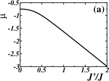
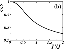
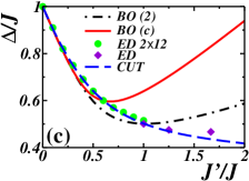
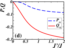
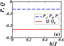
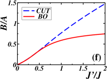
Figure 2: (color online) Properties of the two–chain ladder as a function of coupling ratio $J^{\prime}/J$ at $h$ = 0 = $T$. (a) Chemical potential $\mu$. (b) Singlet condensation fraction $\overline{s}\equiv\langle s\rangle$. (c) Spin gap $\Delta$: bond–operator data from Eqs. (13)–(20) ($BO(c)$, red, solid line); bond–operator data without $P,Q,m$ ($BO(2)$, black, dot–dashed line); ED data for 2$\times$12 system ($ED\;2\!\times\!12$, green circles); ED data extrapolated to an infinite ladder ($ED$, violet diamonds); data from Continuous Unitary Transformations ($CUT$, blue, dashed line). (d) Triplet correlations $P$ and $Q$. (e) $P$ and $Q$ for $J^{\prime}/J=1$, shown as functions of field at $T=0$. (f) Spin correlation ratio $B/A$ (see text), comparing bond–operator and CUT results.

III Zero–temperature ladder physics

III.1 Bond–operator description

An analysis of the physical content of Eqs. (13)–(20) begins by considering the qualitative description of the spin ladder at zero temperature and zero field. The parameter governing the extent of quantum fluctuations away from the limit of decoupled dimers, in which the bond–operator approach is exact, but trivial, is the ratio $J^{\prime}/J$ between the exchange interactions on the chain and rung bonds. The essential picture is a condensate of rung singlets, which are separated by an energy gap of $J$ from the (local) rung triplet states. These form a condensate in the true sense of the word, its coherence mediated by the hopping processes of virtual triplet excitations (the quantum fluctuations) along the ladder.rsb The effective chemical potential $\mu$ (Sec. II) is the parameter fixing the band center of the triplet magnon modes, and the singlet condensate fraction $\overline{s}$ appears also in the effective band width.

Figure 2(a) shows the evolution of $\mu$ as a function of $J^{\prime}/J$; because the dominant contributions to the integrals in the mean–field equations (13)–(20) are given by those $k$ values close to $\pi$, increasingly negative values of $\mu$ are required to maintain a suitable gap $\Delta_{\alpha}=\omega_{\pi,\alpha}$ as $J^{\prime}$ is raised (at $h=0$, the three modes $\alpha$ are degenerate). The singlet condensation fraction $\overline{s}$ [Fig. 2(b)] decreases from precisely unity in the decoupled limit to values of order 80% beyond the isotropic point ($J^{\prime}/J=1$), suggesting a rather high level of singlet condensation even far from the strongly dimerized limit. The gap of the spin ladder is shown in Fig. 2(c), where the bond–operator technique in its simplest, “second–order” formrgrs is compared with its complete form, and also with data obtained by other techniques. ED data for a 2$\times$12 ladder was taken from Ref. [rrtr, ] and that for the extrapolation to an infinite ladder from Ref. [rbdrs, ]. The CUT technique, while perturbative, affords a systematic means of proceeding to very high order,rksgu and can be seen to provide extremely accurate results over a wide range of $J^{\prime}/J$ for a gapped system (i.e. one with a short correlation length) such as the two–chain ladder.

Within the bond–operator description, large quantitative errors are inevitable at $J^{\prime}>J$, where the framework loses its validity: the gap begins to rise again as a consequence of the band center increasing while $\overline{s}$ falls with $J^{\prime}$ [Fig. 2(b)]. Although the gap prediction is accurate only at small $J^{\prime}/J$, the second–order approximation delivers serendipitously good agreement with the exact result precisely at the isotropic point, where $\Delta_{\rm BO}^{(2)}(1)=0.503J$ while $\Delta_{\rm ED}^{\infty}(1)=0.501J$. Although the inclusion of the expectation values $P$ and $Q$ was addressed in Ref. [rgrs, ], a missing factor of 3 for the triplet mode degeneracy caused errors in the results for all quantities. In combination with the above numerical coincidence, this led to rather little attention being paid to the $P$ and $Q$ terms in the literature. Their qualitative importance will become clear in Secs. IV and V. Quantitatively, in fact the complete bond operator result at the isotropic point is $\Delta_{\rm BO}^{(c)}(1)=0.640J$, a value which is close to half–way between the second– and third–order approximations to the gap obtained in a strong–dimerization expansion.rrtr Thus one may conclude that the results obtained from Eqs. (13)–(20) are essentially optimal within the bond–operator framework, and that this is by its nature limited to be quantitatively accurate only up to $J^{\prime}/J\simeq 0.5$. The qualitative physics of the spin ladder may, however, be captured for considerably higher values of the coupling ratio.

At finite fields but zero temperature, the three magnon bands are split by the Zeeman effect, the uniform linear decrease of the entire $+$ branch and increase of the $-$ branch with a slope determined by the $S=1$ nature of the magnons and by the $T=0$ $g$–factor. The zero–field gap is an important quantity because it determines the critical field required to render the lowest mode gapless, and thus to drive the system into the Luttinger–liquid regime at the lowest temperatures.

III.2 Spin correlations

Turning to the interdimer correlations $P$ and $Q$ at zero field and temperature, the evolution of the two quantities as a function of $J^{\prime}/J$ is shown in Fig. 2(d). Their negative sign is a consequence of the relative phase of the triplets. While the triplet hopping term $P$ obviously remains rather small for all ratios, the pair–creation term $Q$ constitutes a very significant quantum fluctuation contribution even at moderate values of $J^{\prime}/J$. For perspective, in the isotropic ladder ($J^{\prime}/J=1$) one finds that each of the three components [$Q$ appears twice (12)] has a value of order 0.23; given that $\overline{s}=0.83$ for $J^{\prime}/J=1$ [Fig. 2(b)], it is largely the $Q$ terms which exhaust the relevant sum rules. The dominance of the triplet pair–creation term found here is fully consistent with studies of the $t$–$J$ ladder.rsrz

Figure 2(e) illustrates the initially non–intuitive result that the zero–temperature triplet correlation functions do not vary at all with the applied magnetic field: $P_{+}=P_{0}=P_{-}$ and $Q=Q_{0}$ at all fields, reflecting the unbroken SU(2) spin symmetry of the electronic wave function in the gapped phase. However, it becomes clear by inspection of the mean–field equations (13)–(20) that in fact a finite temperature is required before the applied field can affect either the $P$ and $Q$ terms or the magnetization $m$. This behavior is the topic of Sec. IV.

There is a direct relationship between the quantities $P$ and $Q$ and the interdimer spin correlations $\langle{\vec{S}}_{i}^{l}{\bf\cdot}{\vec{S}}_{i+1}^{l}\rangle=\langle{\vec{S}}_{i}^{r}{\bf\cdot}{\vec{S}}_{i+1}^{r}\rangle\equiv B$: from Eq. (2) it follows that, up to fourth–order corrections, $B=\textstyle{\frac{3}{2}}\overline{s}^{2}(P+Q)$. Further, the on–dimer spin correlation $\langle{\vec{S}}_{i}^{l}{\bf\cdot}{\vec{S}}_{i}^{r}\rangle\equiv A$ is straightforwardly $A=-\textstyle{\frac{3}{4}}\overline{s}^{2}$, which clearly has the required limit as $J^{\prime}/J\rightarrow 0$ and $\overline{s}\rightarrow 1$, and hence the ratio $B/A=-2(P+Q)$. This ratio has been measuredrsgea ; rtu by neutron–scattering studies of (C₅H₁₂N)₂CuBr₄, and the results are consistent with the ratio $J^{\prime}/J\simeq 1/3.9$ deduced for this material (Sec. V). Bond–operator results for $B/A$ are compared in Fig. 2(f) with the CUT analysis of the spin ladder, also presented in Ref. [rsgea, ], over a range of coupling ratios $J^{\prime}/J$. As for the gap, the bond–operator technique delivers quantitative accuracy up to $J^{\prime}/J\simeq 0.5$, while deviations appear and increase beyond this.

Thus the intrinsic nature of the quantum mechanical wave function of the spin ladder, by which is meant the extent of spin correlations across the different bonds, may be deduced directly from the triplet correlations. Their evolution due to quantum fluctuations (this Sec.) and to thermal fluctuations (Sec. IV), as well as the combined effects of both types of fluctuation in a magnetic field, may be followed in the bond–operator approach. This type of analysis may be applied to a number of gapped, low–dimensional quantum spin systems, including the dimerized $S=1/2$ chain Cu(NO₃)${}_{2}\cdot 2.5$D₂Orxbra and the 2D $S=1/2$ system PHCC,rszrb for which systematic measurements of the quantities $J_{ij}\langle{\vec{S}}_{i}\cdot{\vec{S}}_{j}\rangle$ have already been performed.

IV Finite temperatures

Turning now to the situation at finite temperature, there is naturally no explicit expression for a thermal occupation function of hard–core bosons. This problem was addressed for the ladder system in Ref. [rttw, ] by enforcing the local constraint (3) at the global level to obtain an effective partition function for the hard–core boson system. The effective statistics deduced from this expression,

$$n(\omega_{k,\alpha},\beta)=\frac{e^{-\beta\omega_{k,\alpha}}}{1+\sum_{\alpha}z_{\alpha}(\beta)},$$ (21)

where $\beta$ is the inverse temperature and $z_{\alpha}(\beta)=\sum_{k}e^{-\beta\omega_{k,\alpha}}$ is the partition function of mode $\alpha$, were shown in Ref. [rrnmnfkgbsm, ] to give a spectacularly successful description of the thermal band–narrowing and gap enhancement measured in the 3D coupled–dimer system TlCuCl₃. However, it should be emphasized that the global reweighting of the partition function formulated for a spin ladder in Ref. [rttw, ] is entirely dimension–independent, and thus should function equally well for all hard–core boson systems. Indeed the same ansatz has also been used to obtain good descriptions of thermodynamic quantities in the 2D dimerized spin–chain system (VO)₂P₂O₇run and of spectral weights for the excitations of ultra–cold bosonic atoms on a 1D optical lattice.rrsu

It is important to recall the meaning of Eqs. (13)–(20) at finite temperatures. The spectrum of excitations of any Hamiltonian is a temperature–independent quantity, and the temperature is responsible only for driving changes in the weights with which given modes are occupied. These spectral weights are represented by the dynamic structure factor $S({\vec{k}},\omega,T)$, which can be measured by INS. The bond–operator approach delivers an effective description of the one–magnon sector of the dynamical structure factor, in the form of a peak position for each of the (field–split) magnon branches. Changes in these peak positions as a function of temperature are in fact a statement of the leading thermal effects on the spectral–weight distribution: the key result of Ref. [rrnmnfkgbsm, ] is that thermal shifts in the peak positions by factors of up to 3 are not accompanied by thermal broadening of the excitations over the same energy width. That the magnon modes remain coherent shows that their spectral–weight shifts are a true many–body effect governed by the overall band structure and by their hard–core statistics. These features are captured over the full range of temperatures (up to $T\sim J$) in the bond–operator framework with Eq. (21).

Heuristically, a band–narrowing effect arises because, while the temperature does not alter the magnetic exchange interactions, thermal occupation of some dimer sites by triplets acts to block the motion of a propagating test triplet due to the local hard–core constraint (3). This is reflected in the fact that the effective occupation function for mode $\alpha$ (21) involves explicitly terms due to all three magnon branches, thus encoding a form of inter–branch exclusion. In the self–consistent solution of the mean–field equations, an increase in ${\tilde{n}}(\omega_{k,\alpha})$ with increasing temperature causes a drop in all of the quantities $\overline{s}$, $P$, and $Q$. The physical interpretation of this effect is a suppression both of on–dimer singlet condensation and in the coherence of interdimer fluctuation processes, which results in a narrowing of the magnon bands and consequent increase in the gap. While such an effect is also obtained with bosonic statistics, only the effective occupation function of Eq. (21) takes into account correctly the number of available hard–core boson states of the system.

In this section, the qualitative physics of the two–chain spin ladder at finite fields and temperatures is illustrated using the isotropic coupling ratio, $J^{\prime}/J=1$. This value is not chosen for any special reason: it is already clear from the previous section that the bond–operator description is not quantitatively accurate beyond $J^{\prime}/J=0.5$, and it is not the case that some of the qualitative effects become stronger as the coupling ratio increases (indeed, as shown in Sec. V, the converse is true for certain quantities). The choice is simply a good representative value for a ladder away from the strongly dimerized limit, and serves as an instructive counterpoint to the results presented in Sec. V for $J^{\prime}/J=1/3.9$ (a value which is effectively in this limit).

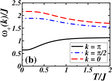
Figure 3: (color online) (a) Magnon bands $\omega_{\alpha}(k)$, shown for the isotropic ladder at $T/J=0.1$ and in a field $h/J=0.5$. (b) Thermal evolution of the band maximum, center, and minimum for a spin ladder with $J^{\prime}/J=1$ and $h=0$.

IV.1 Magnon dispersion

Figure 3(a) serves first as a reminder of the magnon band structure: there are three branches, which all have a minimum at the antiferromagnetic wave vector $k=\pi$ and which are similar in shape and splitting. However, for a ladder beyond the strongly dimerized limit ($J^{\prime}\ll J$), and at finite fields and temperatures, these branches are not symmetrical (in $k$) about a band center, they do not have exactly the same line shape, and their separation is not exactly the bare Zeeman splitting defined in Sec. IIIA; all of these facts can be read from Eqs. (9)–(12).

.    

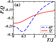
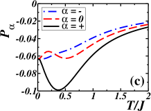
Figure 4: (color online) (a) Triplet correlations $P$ (blue, dashed) and $Q$ (red, solid) as functions of temperature for $J^{\prime}/J=1$ and $h=0$. $P$ is shown multiplied by a factor of 4 to illustrate its relative thermal renormalization. (b) Triplet correlations $P_{+}$, $P_{0}$, and $P_{-}$ shown as functions of field at $T/J=0.1$. (c) $P_{+}$, $P_{0}$, and $P_{-}$ and (d) $Q$ and $Q_{0}$ as functions of temperature for $J^{\prime}/J=1$ and $h/J=0.5$.

Considering first the case with no magnetic field, Fig. 3(b) illustrates the thermal band–narrowing effect by showing for the isotropic ladder the $T$–dependence of the band maximum ($k=0$), band minimum ($k=\pi$), and band center defined as the mode energy at $k=\pi/2$. The suppression of hopping begins when $T$ becomes similar to the gap, and the effect saturates when $T$ exceeds $J$. The form of the thermal renormalization, and of the consequent growth of the gap with temperature, is exactly analogous to the results obtained for TlCuCl₃ in Ref. [rrnmnfkgbsm, ]. As noted above, $\omega_{k,\alpha}$ obtained from the bond–operator formalism is the peak position at finite temperture of the one–magnon spectral weight of the spin ladder, a quantity not yet available from any numerical approaches. However, some recent attempts to compute effective magnon spectra for quantum magnets at finite temperatures, specifically ED calculations for short, dimerized (gapped) $S=1/2$ chainsrml and real–time DMRG calculations for gapless $S=1/2$ Heisenberg chains,rbsw suggest that further progress can be expected in this direction.

The evolution of the zero–field triplet correlations $P$ and $Q$ corresponding to this band–narrowing is shown in Fig. 4(a). The two quantities have contrasting behavior: while finite temperatures act only to suppress pair–creation processes (i.e. rendering these less coherent), the hopping correlations show an initial rise, or thermal enhancement of such processes, before thermal decoherence becomes the dominant effect. Here the terms “coherence” and “decoherence” are used in the sense of Sec. III, the former to indicate the intrinsic correlations driven by quantum fluctuations (which depend on $J^{\prime}/J$, Fig. 2) and the latter to indicate the suppression of these correlations by thermal fluctuations.

At finite fields and temperatures, the full complexity of the system becomes visible, with effects appearing which are not present at finite $h$ or $T$ alone. Figures 4(c) and (d) show the thermal evolution of the triplet correlation functions at finite $h$: $P_{+}$ is strongly and $Q$ weakly enhanced at small fields, before thermal decoherence takes over; $P_{-}$ is generally anticorrelated to $P_{+}$, but has no mechanism for initial suppression corresponding to the enhancement of $P_{+}$; $P_{0}$ shows a non–monotonic evolution as a consequence of the competing effects of coupling to $P_{+}$, the field scale, and the two opposing forms of thermally driven behavior [Fig. 4(a)]; $Q_{0}$ shows the same weak anticorrelation to $Q$, followed by thermal decoherence [Fig. 4(d)]. The correlation functions vary somewhat predictably with $h$ when $T$ is fixed, as shown in Fig. 4(b), although it should be noted that the flat line is $P_{-}$, while $P_{0}$ is the function which drops more strongly as $P_{+}$ is enhanced. This result can be understood by considering the corresponding temperature in Fig. 4(c).

It is important to note at this point that it is not particularly meaningful to discuss temperatures $T$ in excess of, or even on the order of, the rung coupling scale $J$. At these temperatures, the concept of the rung singlet and triplets as well–defined states of the two rung spins breaks down, and it is more appropriate to consider these spins separately. Even at temperatures considerably below $J$, magnon excitations become broad functions in the space of energy and wave vector: the complex question of this intrinsic line width in a gapped quantum magnet has been considered only at the semiclassical level,rds and more microscopically in some limiting cases,re but is not addressed within the bond–operator framework at the current level of approximation. Thus the data up to $T=2J$ shown in Figs. 3 and 4 are to be taken only as an example of the physics encoded in the mean–field equations, and all of the figures to follow will be cut at $T=J$. For those concerning the critical properties of the ladder near the field–driven crossover to the Luttinger–liquid phase, further caveats will be necessary.

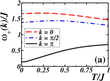
Figure 5: (color online) (a) Band–narrowing effects for the isotropic ladder at $h/J=0.5$. (b) Gap–curvature effects for the band minimum of the three triplet branches, illustrated for the isotropic ladder with $T/J=0.1$.

The thermal renormalization of the triplet band width at finite field is shown in Fig. 5(a). The effect of the field is to reduce further the symmetry of the band edges, causing an initial upward trend at the upper edge as thermal fluctuations allow the polarizing effect of the field to operate. Analogous to the effects visible in Figs. 3 and 4, this behavior is reversed at higher temperatures, as $T$ competes with $h$, resulting in an overall downward trend of the band center. The consequences for the mode gaps as a function of field at finite $T$ are shown in Fig. 5(b): here one may regard the 0–mode curvature as an indication of generic thermal effects (increased net energy), on top of which the additional contributions contained in the $P$ and $m$ terms in Eqs. (9) and (11) act against this curvature for the upper–mode gap, giving a rather straight field–dependence, but an enhanced curvature away from gap closure of the lower mode. This reflects the basic physical phenomenon that the lower mode absorbs most of the thermally excited magnons at finite $T$ and $h$, and is thus the most strongly renormalized; the necessary deviation from Zeeman splitting is contained in the $P$ and $m$ terms.

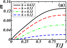
Figure 6: Magnetization $m$ as a function of $T$ for four different magnetic fields (a) and as a function of $h$ for three different temperatures (b).

IV.2 Thermodynamic properties

It is instructive to consider the magnetization $m$ to understand its evolution with field and temperature, and hence how it affects the magnon dispersion branches. For a fixed field as a function of temperature [Fig. 6(a)], $m$ is non–monotonic, first rising as a consequence of the thermally excited states which become available to react to the field, but becoming maximal as $T$ approaches $J$. The low–temperature rise is clearly of activated form, the gap diminishing as the field is raised. Only close to the critical field which closes the gap ($h/J=0.64$ in the isotropic ladder) does the exponential form turn over to a power law, which in 1D is expected to be a square root as a function of temperature at very low $T$. The value of $m$ at the maximum is clearly an almost linear function of the field which is polarizing the available triplet states. The high–$T$ behavior, found also in extensive TMRG studies of $m(h,T)$,rwy sets in when $T$ competes with the interaction energy scales of the system, suppressing not only triplet propagation and the polarized moment, but also dimer singlet formation itself.

Figure 6(b) shows $m$ as a function of $h$ for different temperatures. In general, both the number of states becoming available and the field which is able to polarize them give contributions to $m$. At low $T$ the response is activated and the dominant contribution is due to the field. At high $T$, for which $T/J=0.5$ is already sufficient, $m$ becomes an entirely linear function of $h$: here the temperature ensures a large number of available states, and these are polarized by whatever field is applied. This physics, also illustrated below in Figs. 9(e) and (f), constitutes a regime in which the gap renormalization [of the type shown in Fig. 5(b)] is also completely linear. This results in a “pseudo–Zeeman” behavior of the mode minima in an applied field, where the gaps evolve linearly but with a slope reduced from the conventional, zero–temperature value by the $P_{+}-P_{-}$ and $m$ terms in Eqs. (9) and (11). It is possible that this behavior has been misinterpreted in some previous analyses of low–dimensional quantum magnets, for example as a $T$–dependent $g$–factor.

At low temperatures one finds that $m\simeq{\textstyle\frac{1}{2}}(P_{-}-P_{+})$, and thus that the two contributions to non–Zeeman behavior of the gap are essentially equal. This value of $m$ can be regarded as the quantum–fluctuation contribution to the magnetization. As $T$ is increased, $m$ increases compared to $|P_{+}-P_{-}|$, until at high temperatures it is exponentially greater: while $m$ is enhanced by thermal population effects, there is no such contribution to $|P_{+}-P_{-}|$, which indeed is suppressed at high temperatures [Fig. 4(c)].

In dimensions of 2 and higher, it is of great interest to investigate the temperature–dependence of the critical field $h_{c}$, the field which closes the excitation gap of the quantum spin system, driving a quantum phase transition. The quantity $h_{c}(T)-h_{c}(0)$ encapsulates the critical properties of the theory, and has been analyzed in detail for the higher–dimensional cases, where the transition is in the Bose–Einstein universality class.rgrt In this case, the transition is from a (singlet–based) quantum disordered state to an ordered magnetic one, the order parameter being the transverse (staggered) moment. The low–temperature behavior of the phase–transition line should have the scaling form $h_{c}(T)-h_{c}(0)=AT^{d/2}$, where A is a constant, $d$ is the spatial dimensionality of the system, and the denominator 2 in the exponent enters from the quadratic dispersion of the free hard–core bosons ($\omega\propto k^{2}$) at the transition.

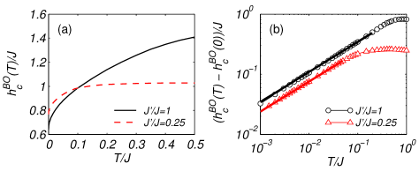
Figure 7: (a) Critical magnetic field $h_{c}^{\rm BO}$ required to close the effective spin gap of ladders with coupling ratios $J^{\prime}/J=1$ and 0.25 at finite temperatures. (b) $h_{c}^{\rm BO}(T)-h_{c}^{\rm BO}(0)$ on logarithmic axes to illustrate square–root scaling (solid lines).

In a 1D system, there is no ordered phase or order parameter, and indeed no transition: $h_{c}(T)$ marks a crossover to the Luttinger–liquid regime.rsss ; rcrct Under these circumstances, the definition of a quantity $h_{c}(T)$ may not be unique. The crossover has nevertheless been found to have a very clear signature both in experimental measurements of the thermodynamic properties of (C₅H₁₂N)₂CuBr₄ and in numerical studies of the magnetization $m(h,T)$. In measurements of the magnetocaloric effect,rcrct its location was deduced from the minima and maxima in $m(T)$ through the condition $\partial m/\partial T|_{h}=0$, while in TMRG calculationsrwy it was taken from the maximum in $\partial m/\partial h$. The quantity $h_{c}^{\rm BO}(T)$ investigated in the bond–operator description is that value of the field where the maximum of the finite–temperature, one–magnon spectral function is moved to zero frequency, and therefore does not necessarily have a direct relation to the crossover field (which is dictated by the lowest level in the excitation spectrum): it is rather a statement about the reaction of the spectral–weight function to thermal flucutations, which may be very different in 1D from the higher–dimensional cases. For practical purposes, $h_{c}^{\rm BO}(T)$ marks the limit of applicability of the bond–operator formalism at the level of Sec. II, which cannot be used for the gapless phase without extensive modification. At $T=0$, the quantity $h_{c}=h_{c}^{\rm BO}(0)$ is the same crossover field as that obtained from all other definitions.

The critical field $h_{c}^{\rm BO}(T)$ is shown in Fig. 7(a) for the isotropic ladder, and by way of comparison also for a ladder with coupling ratio $J^{\prime}/J=1/4$. At low temperatures, both curves have a very rapid increase with $T$: the logarithmic fit in Fig. 7(b) reveals this singular behavior to have precisely the square–root form obtained from the analysis above with $d=1$. Thus the effect of thermal fluctuations on the low–temperature spectral function is indeed dramatic. Beyond the critical regime, $h_{c}^{\rm BO}(T)$ becomes flatter at higher temperatures, meaning that the maximum of the excitation spectrum becomes rather temperature–insensitive. A slight decrease is visible for $J^{\prime}/J=1/4$ as the system approaches the “breakdown” regime $T\sim J$, where the theory contains diminishing energy scales [visible in the magnon bands (Figs. 3 and 5) and in the magnetization (Fig. 6)]. Returning to the critical regime, while it may be taken to exist over a temperature range of order $0.2J$ in the isotropic ladder, it is clearly correspondingly narrower for smaller coupling ratios ($T/J\sim 0.05$ at $J^{\prime}/J=1/4$). This narrow 1D critical regime is precisely that part cut off by 3D coupling even in very weakly interacting, quasi–1D ladder systems such as (C₅H₁₂N)₂CuBr₄.

A further thermodynamic quantity which can be computed in this framework is the magnetic specific heat. Obtained from the second temperature derivative of the effective hard–core boson free energy, this can be expressed in the form

$$C_{m}(T)\!=\!\!\sum_{k,\alpha}\!\frac{\beta^{2}\omega_{k,\alpha}^{2}e^{-\beta\omega_{k,\alpha}}}{1+\sum_{\alpha}\!z_{\alpha}(\beta)}\!-\!\left(\frac{\beta\omega_{k,\alpha}e^{-\beta\omega_{k,\alpha}}}{1+\sum_{\alpha}\!z_{\alpha}(\beta)}\right)^{2}\!\!\!.$$ (22)

Consideration of the magnetic specific heat is deferred to Sec. V, where it is discussed in the context of a direct experimental comparison.

V $\rm\bf(C_{5}H_{12}N)_{2}CuBr_{4}$

Having understood in full the physics contained in the complete mean–field equations, one may turn to the nearly ideal spin–ladder material (C₅H₁₂N)₂CuBr₄. Fits to the magnon bands, of the type shown in Fig. 3(a), were performed in Ref. [rbtins, ] and will not be repeated here. In the bond–operator framework they give $J=13.07$ K, $J^{\prime}=3.35$ K, and hence a coupling ratio within the spin ladders of $J^{\prime}/J=1/3.9$.rbtins In this strongly dimerized regime (sometimes referred to as the “strong–coupling” regime), the bond–operator description is extremely accurate (Sec. III).

The real material has a number of complications which may affect the accuracy of a detailed comparison between this theoretical description and experimental measurement on levels of up to 5%. For the present purposes, the most important is the anisotropy in the $g$–factor,rpsw ; rcea which enters the comparisons between thermodynamic measurements (most performed with ${\vec{H}}\parallel{\hat{a}}$) and INS dispersion relations (${\vec{H}}\parallel{\hat{b}}$). The value chosen here to reproduce $H_{c}=6.99$ T, $g=2.12$, is close to the average in the $(ab)$–plane of the system. Among the other materials questions, one is the weak interladder coupling mentioned in Sec. I, which is approximately 3% of $J$;rbtins another is a detectable magnetostriction effect (changes of $J$ and $J^{\prime}$ with applied field) of order 1%, which becomes relevant when comparing the low– and high–field gapped regimes;rbtins a third is a spin anisotropy, or a breaking of SU(2) spin symmetry of as–yet undetermined origin, which a recent ESR investigationrcea has estimated as high as 5% of $J$. While a spin anisotropy can be included in the current framework when enough information becomes available, the high–field regime is not the focus of the current manuscript and the 3D nature of the material is not of prime importance while the system has a robust spin gap, meaning at all fields below where $h$ enters the critical regime close to $h_{c}$.

In this section, results are presented only for 1D ladders with coupling ratio $J^{\prime}/J=1/3.9$. Fig. 8 shows the triplet correlations $P$ and $Q$ which assist a qualitative understanding of the ladders in (C₅H₁₂N)₂CuBr₄. Figure 9 shows the magnetization and one–magnon band structure of these ladders at finite fields and temperatures, giving direct experimental predictions. Figure 10 considers the thermodynamics of these ladders through the magnetic specific heat, including a direct experimental comparison and quantitative reproduction of published data for this quantity.

.    

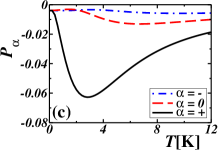
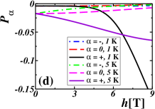
Figure 8: (color online) Triplet correlation functions for the ladders of (C₅H₁₂N)₂CuBr₄ at different temperatures and applied magnetic fields. (a) $P_{\alpha}$ for $\alpha=+,0,-$ as functions of temperature at a field of 1 T. (b) $Q_{0}$ and $Q_{+-}=Q$ as functions of temperature at fields of 1 T and 6 T. (c) $P_{\alpha}$ at a field of 6 T. (d) $P_{\alpha}$ as a function of field for temperatures of 1 K and 5 K.

Beginning with the triplet correlations, the quantities $P_{\alpha}$ and $Q_{\alpha}$ are shown in Fig. 8 for ladders with $J^{\prime}/J=1/3.9$. It is clear in Fig. 8(a) that the general enhancement of hopping correlations by a finite temperature is large in strongly dimerized ladders, and that the scale for thermal decoherence to dominate the correlation physics of (C₅H₁₂N)₂CuBr₄ is $T\sim 10$ K. The same quantity shown not at low field but close to the critical point [Fig. 8(c)] emphasizes the very strong effect which the field can have on the enhancement of $P_{+}$ in this regime of $J^{\prime}/J$ [note the different scales in panels (a) and (c)]. The triplet pair–creation correlation function $Q_{\alpha}$, however, depends strongly on neither field nor temperature, being sensitive only to the thermal decoherence effect [Fig. 8(b)]. As a function of the magnetic field [Fig. 8(d)], splitting of the hopping correlations in the three branches requires significant field strengths at low temperatures, where thermal occupations are activated, but the effect is nevertheless very strong on approaching the critical region. By contrast, at higher temperatures where states in all branches are available, all applied fields are capable of splitting the branches but the effect is rather modest.

.    
.    

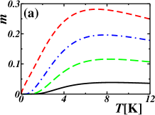
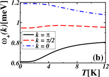
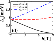
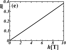
Figure 9: (color online) Calculations for (C₅H₁₂N)₂CuBr₄ ladders at finite temperature and magnetic field: as functions of temperature, (a) magnetization $m$ for fields of 1 T (black, solid line), 3 T (green, long–dashed line, 5 T (blue, dot–dashed line), and 6.99 T (red, dashed line) and (b) magnon band width at a field of 2 T; as functions of the applied magnetic field, magnetization $m$ (c,e) and gaps $\Delta_{\alpha}$ (d,f) at temperatures of 1 K (c,d) and 10 K (e,f).

Figure 9 turns to some of the observables of the ladder system. The magnetization as a function of temperature over a range of fixed magnetic fields is shown in Fig. 9(a): initial activated behavior dictated by the spin gap leads to a peak around $T\sim J/2$ and then to the slow decrease indicative of the loss of coherence in the magnetic sector. These features are qualitatively similar to those of the magnetic specific heat, shown in Fig. 10, but differ in magnitude because $m$ increases as the system approaches the critical field [Fig. 6(a)]. Figure 9(b) shows the thermal band–narrowing effect of Figs. 3(b) and 5(a), illustrated for a magnetic field of 2 T. This phenomenon was explained in Sec. IV, and INS measurements are expected shortly. Data for the magnetization $m$ and for the gap $\Delta_{\alpha}$ of each mode as functions of the applied field, at temperatures equivalent to 1 K and 10 K, are shown in Figs. 9(c)–(f). The magnetization at 1 K [Fig. 9(c)] shows the activated behavior visible at lower temperatures in Fig. 6(b), and the gap of the low–lying mode [Fig. 9(d)] has a significant curvature of the type shown in Fig. 5(b). By contrast, the 10 K data are well in the high–temperature limit discussed in Sec. IV, where the ready availability of thermally excited states leads to a linear magnetization [Fig. 9(e)] and to the pseudo–Zeeman form of the mode gaps as functions of temperature [Fig. 9(f)]. It should be stressed, however, that in experiment it is somewhat unlikely that clearly defined magnon excitations would still be visible at temperatures as high as 10 K, due to extensive thermal broadening of the response function. If one considers temperatures of approximately 5 K, where a definite magnon mode may still be detectable, then these data are rather similar to the forms shown in Figs. 9(e) and (f), albeit with some discernible curvature remaining in $m$ and $\Delta_{+}$.

The most directly measurable and perhaps informative single thermodynamic quantity is the magnetic specific heat. Detailed measurements performed on (C₅H₁₂N)₂CuBr₄ over the full range of temperatures, and of applied magnetic fields in both the gapped (quantum disordered) and gapless (Luttinger–liquid) phases, are presented in Ref. [rcrct, ]. The experimental results were compared with somewhat numerically demanding ED and DMRG studies of ladders with the same coupling ratio, and also to a bond–operator approximation in the gapped regime and a Bethe–Ansatz approximation in the gapless one. The same behavior of the magnetic specific heat as a function of field and temperature has also been demonstrated in TMRG studies of ladder thermodynamics,rwy but has not been computed explicitly for the parameters of (C₅H₁₂N)₂CuBr₄.

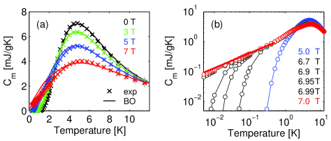
Figure 10: (color online) (a) Magnetic specific heat of (C₅H₁₂N)₂CuBr₄ at magnetic fields of 0 T (black, uppermost peak), 3 T (green, second peak), 5 T (blue, third peak) and 7 T (red, lowest peak). Solid lines are given by the complete bond–operator theory, while crosses show experimental data presented in Ref. [rcrct, ]. (b) Specific–heat data from bond–operator theory, shown on logarithmic axes to illustrate the approach to a low–$T$ square–root form as $h\rightarrow h_{c}$. The red, solid line marks a slope of 1/2.

The magnetic specific heat given by the complete bond–operator approach is shown in Fig. 10(a) for fields corresponding to 0 T, 3 T, 5 T, and 7 T, along with experimental measurements made at the same fields.rcrct In the regime with a robust spin gap, the specific heat shows exponential activation at low temperatures, followed by a peaking at $T\sim J/2$. The activation gap decreases as the field is raised, resulting in more weight at lower temperatures and a drop in the peak height. By contrast, the critical field which closes the triplet gap in a single (C₅H₁₂N)₂CuBr₄ ladder is 6.99 T, and hence the system shows gapless behavior at 7 T; note that while the bond–operator description is no longer valid at $h>h_{c}$ for $T=0$, the rapid rise of $h_{c}^{\rm BO}$ with temperature shown in Fig. 7 ensures that the gapless nature of the excitations becomes a numerical problem only at temperatures two orders of magnitude below those shown in Fig. 10(a). As the field approaches $h_{c}$, the peak height at $T\sim J/2$ continues to fall; both this peak and the high–$T$ decrease are features sensitive not to the gap but to the center and upper edges of the excitation band.

The low–$T$ form of the specific heat in the gapless regime is a power law, and the power in a spin ladder at the critical field is 1/2. Figure 10(b) shows specific–heat data obtained as $h$ approaches $h_{c}$ from below: clearly a square–root dependence is obtained, but only for fields extremely close to the critical value (cf. Ref. [rlea, ]). That even differences of 0.01 T can have a significant impact on the form of thermodynamic quantities indicates at the theoretical level the possibility that the quantum critical regime may be extremely narrow, and at the experimental level the need for exquisite accuracy in the measurement of critical properties.

The data computed from Eqs. (13)–(20), represented as lines in Fig. 10(a), is in perfect quantitative agreement with essentially every feature of the 0 and 3 T experimental data, and shows only the most minor deviations at 5 T. There is no separate scale factor for each curve, i.e. as already stressed above there are no free parameters in the theory. Only on the critical line, at the very limit of applicability of the bond–operator framework, are some small but systematic discrepancies noticeable: specifically, the complete bond–operator result gives a peak height (around 5 K) which is marginally too low, and this missing weight appears to be present around temperatures of 2 K. However, the results of Fig. 10(b) indicate that extreme caution is required before ascribing this to a failure of the bond–operator description, as the true proximity of the experimental measurements to the critical field is accurate perhaps only to within 0.05 T.

The bond–operator approximation applied in Ref. [rcrct, ] used the same effective magnon statistics as here, but not the $P$, $Q$, and $m$ terms; the same qualitative form of error was found when $h\rightarrow h_{c}$ as in Fig. 10(a), but it was very much larger (of order 15% in the peak height). Figure 10(a) makes clear that the self–consistent inclusion of these terms results in a very significant correction of this error. Thus the complete bond–operator framework is highly accurate even at the very limit of its regime of applicability and even in one dimension. It was noted in Ref. [rcrct, ] that some degree of error may be introduced by the treatment of the hard–core constraint (3): while the total number of states is correct, global application of the constraint may result in some of these states not being penalized sufficiently for the fact that they violate the constraint at the local level. Extra weight would then be expected not in the peak but at lower energies, perhaps resulting in the apparent persistence of the low–$T$ critical (power–law) regime to artificially high temperatures. However, the results in Fig. 10 show that these errors are at the percent level even for $h=h_{c}$, and that the complete bond–operator theory is capable of a fully quantititively accurate description of all features of the gapped, strongly dimerized spin ladder.

A more explicit summary statement on the accuracy of the complete bond–operator treatment for the two–chain spin ladder, drawn from all of the results above, is the following: it is extremely high, meaning quantitative agreement within a few percent when compared to numerical results (particularly DMRG for the spectrum and TMRG for thermodynamics) for the strongly dimerized regime $J\gg J^{\prime}$. This level of agreement, which is achieved with no adjustable parameters, extends to $J^{\prime}\simeq J/2$ and applies to all physical observables computed here (spin correlations, magnon spectra, thermodynamic quantities). Quantitative deviations from percent levels of accuracy become noticeable as $J^{\prime}/J$ is further increased towards the isotropic case, a result not at all surprising in view of the expected regime of applicability of the bond–operator method, and the type of quantum fluctuations which it is designed to capture. In the isotropic ladder, where the qualitative physics of the system is nevertheless very well described within the bond–operator approach (hence its use for illustrative purposes in Sec. IV), the level of quantitative error as judged from the interdimer spin correlations and the zero–field spin gap is of order 20%.

VI Summary

A complete version of the bond–operator theory for the spin ladder has been developed, which captures all of the relevant physics of the quantum disordered system, at all temperatures and all magnetic fields up to the closure of the spin gap. [At this point the magnon excitations fractionalize into spinons and a Luttinger–liquid description is appropriate.] At the heart of the finite–temperature framework is a global ansatz for the effective exclusion statistics of the magnon excitations, which are hard–core bosons. Among the phenomena described with quantitative accuracy and with no free parameters are the spin correlations, the thermal evolution of the magnon bands, and their thermodynamic properties. Extensive comparison becomes possible with existing data for the spin–ladder material (C₅H₁₂N)₂CuBr₄, and predictions are made for forthcoming experiments which will investigate the thermal renormalization of the magnon excitations. The same treatment is also applicable to calculate finite–temperature properties in the quantum disordered phases of other coupled–dimer systems of any dimensionality.

- (1) Z. Hiroi, M. Azuma, M. Takano, and Y. Bando, J. Solid State Chem. 95, 230 (1991).
- (2) see E. Dagotto and T. M. Rice, Science 271, 618 (1996), and references therein.
- (3) S. R. White, R. M. Noack, and D. J. Scalapino, Phys. Rev. Lett. 73, 886 (1994).
- (4) N. Okazaki, K. Okamoto, and T. Sakai, J. Phys. Soc. Jpn. 69, 2419 (2000).
- (5) V. Gritsev, B. Normand, and D. Baeriswyl, Phys. Rev. B 69, 094431 (2004).
- (6) M. Sigrist and A. Furusaki, J. Phys. Soc. Jpn. 65, 2385 (1996).
- (7) C. A. Hayward and D. Poilblanc, Phys. Rev. B 53, 11721 (1996).
- (8) H. H. Lin, L. Balents, and M. P. A. Fisher, Phys. Rev. B 56, 6569 (1997).
- (9) E. Dagotto, J. Riera, and D. Scalapino, Phys. Rev. B 45, 5744 (1992).
- (10) M. Sigrist, T. M. Rice, and F. C. Zhang, Phys. Rev. B 49, 12058 (1994).
- (11) see T. Giamarchi, Ch. Rüegg, and O. Tchernyshyov, Nature Physics 4, 198 (2008), and references therein.
- (12) Ch. Rüegg, A. Furrer, D. Sheptyakov, Th. Strässle, K. W. Krämer, H.–U. Güdel, and L. Mélési, Phys. Rev. Lett. 93, 257201 (2004).
- (13) Ch. Rüegg, B. Normand, M. Matsumoto, A. Furrer, D. McMorrow, K. Krämer, H.–U. Güdel, S. Gvasaliya, H. Mutka, and M. Boehm, Phys. Rev. Lett. 100, 205701 (2008).
- (14) T. Nikuni, M. Oshikawa, A. Oosawa, and H. Tanaka, Phys. Rev. Lett. 84, 5868 (2000).
- (15) Ch. Rüegg, N. Cavadini, A. Furrer, H.–U. Güdel, K. Krämer, H. Mutka, A. Wildes, K. Habicht, and P. Vorderwisch, Nature 423, 62 (2003).
- (16) M. Troyer, H. Tsunetsugu, and D. Würtz, Phys. Rev. B 50, 13515 (1994).
- (17) Ch. Rüegg, B. Normand, M. Matsumoto, C. Niedermayer, A. Furrer, K. Krämer, H.–U. Güdel, Ph. Bourges, Y. Sidis, and H. Mutka, Phys. Rev. Lett. 95, 267201 (2005).
- (18) B. R. Patyal, B. L. Scott, and R. D. Willett, Phys. Rev. B 41, 1657 (1990).
- (19) B. C. Watson, V. N. Kotov, M. W. Meisel, D. W. Hall, G. E. Granroth, W. T. Montfrooij, S. E. Nagler, D. A. Jensen, R. Backov, M. A. Petruska, G. E. Fanucci, and D. R. Talham, Phys. Rev. Lett. 86, 5168 (2001).
- (20) S. Sachdev, T. Senthil, and R. Shankar, Phys. Rev. B 50, 258 (1994).
- (21) C. A. Hayward, D. Poilblanc, and L. P. Levy, Phys. Rev. B 54, R12649 (1996).
- (22) R. Chitra and T. Giamarchi, Phys. Rev. B 55, 5816 (1997).
- (23) F. Mila, Eur. Phys. J. B 6, 201 (1998).
- (24) T. Lorenz, O. Heyer, M. Garst, F. Anfuso, A. Rosch, Ch. Rüegg, and K. Krämer, Phys. Rev. Lett. 100, 067208 (2008). F. Anfuso, M. Garst, A. Rosch, O. Heyer, T. Lorenz, Ch. Rüegg, and K. Krämer, Phys. Rev. B 77, 235113 (2008).
- (25) Ch. Rüegg, K. Kiefer, B. Thielemann, D. F. McMorrow, V. Zapf, B. Normand, M. B. Zvonarev, P. Bouillot, C. Kollath, T. Giamarchi, S. Capponi, D. Poilblanc, D. Biner, and K. W. Krämer, Phys. Rev. Lett. 101, 247202 (2008).
- (26) B. Thielemann, Ch. Rüegg, K. Kiefer, H. M. Rønnow, B. Normand, P. Bouillot, C. Kollath, E. Orignac, R. Citro, T. Giamarchi, A. M. Läuchli, D. Biner, K. W. Krämer, F. Wolff–Fabris, V. Zapf, M. Jaime, J. Stahn, N. B. Christensen, B. Grenier, D. F. McMorrow, and J. Mesot, Phys. Rev. B 79, 020408(R) (2009).
- (27) M. Klanjšek, H. Mayaffre, C. Berthier, M. Horvatić, B. Chiari, O. Piovesana, P. Bouillot, C. Kollath, E. Orignac, R. Citro, and T. Giamarchi, Phys. Rev. Lett. 101, 137207 (2008).
- (28) B. Thielemann, Ch. Rüegg, H. M. Rønnow, J.–S. Caux, A. M. Läuchli, B. Normand, D. Biner, K. W. Krämer, H.–U. Güdel, J. Stahn, S. N. Gvasaliya, K. Habicht, K. Kiefer, M. Boehm, D. F. McMorrow, and J. Mesot, Phys. Rev. Lett. 102, 107204 (2009).
- (29) T. Barnes, E. Dagotto, J. Riera, and E. S. Swanson, Phys. Rev. B 47, 3196 (1993).
- (30) X. Wang and L. Yu, Phys. Rev. Lett. 84, 5399 (2000).
- (31) S. Trebst, H. Monien, C. J. Hamer, Z. Weihong, and R. R. P. Singh, Phys. Rev. Lett. 85, 4373 (2000).
- (32) C. Knetter, K. P. Schmidt, M. Grüninger, and G. S. Uhrig, Phys. Rev. Lett. 87, 167204 (2001).
- (33) B. Normand, Acta Phys. Pol. B 31, 3005 (2000).
- (34) S. Sachdev and R. Bhatt, Phys. Rev. B 41, 9323 (1990).
- (35) S. Gopalan, T. M. Rice, and M. Sigrist, Phys. Rev. B 49, 8901 (1994).
- (36) M. Matsumoto, B. Normand, T. M. Rice, and M. Sigrist, Phys. Rev. Lett. 89, 077203 (2002); Phys. Rev. B 69, 054423 (2004).
- (37) B. Normand and T. M. Rice, Phys. Rev. B 54, 7180 (1996).
- (38) B. Normand and T. M. Rice, Phys. Rev. B 56, 8760 (1997).
- (39) M. Reigrotzki, H. Tsunetsugu, and T. M. Rice, J. Phys. Cond. Matter 6, 9236 (1994).
- (40) A. T. Savici, G. E. Granroth, C. L. Broholm, D. M. Pajerowski, C. M. Brown, D. R. Talham, M. W. Meisel, K. P. Schmidt, G. S. Uhrig, and S. E. Nagler, Phys. Rev. B 80, 094411 (2009).
- (41) B. Thielemann, Ph. D. thesis, ETH Zurich (2009).
- (42) G. Xu, C. Broholm, D. H. Reich, and M. A. Adams, Phys. Rev. Lett. 84, 4465 (2000).
- (43) M. B. Stone, I. Zaliznyak, D. H. Reich, and C. Broholm, Phys. Rev. B 64, 144405 (2001).
- (44) G. S. Uhrig and B. Normand, Phys. Rev. B 58, R14705 (1998); Phys. Rev. B 63, 134418 (2001).
- (45) A. Reischl, K. P. Schmidt, and G. S. Uhrig, Phys. Rev. A, 72, 063609 (2005).
- (46) H.–J. Mikeska and C. Luckmann, Phys. Rev. B 73, 184426 (2006).
- (47) T. Barthel, U. Schollwöck, and S. R. White, Phys. Rev. B 79, 245101 (2009).
- (48) K. Damle and S. Sachdev, Phys. Rev. B 57, 8307 (1998).
- (49) F. H. L. Essler and R. M. Konik, Phys. Rev. B 78, 100403 (2008); A. J. A. James, F. H. L. Essler, and R. M. Konik, Phys. Rev. B 78, 094411 (2008); W. D. Goetze, U. Karahasanovic, and F. H. L. Essler, unpublished (arXiv:1005.0492).
- (50) E. Čižmár, M. Ozerov, J. Wosnitza, B. Thielemann, K. W. Krämer, Ch. Rüegg, O. Piovesana, M. Klanjšek, M. Horvatić, C. Berthier, and S. A. Zvyagin, unpublished (arXiv:1005:1474).