The role of $P$-wave inelasticity in $J/\psi\to\pi^{+}\pi^{-}\pi^{0}$

Abstract

We discuss the importance of inelasticity in the $P$-wave $\pi\pi$ amplitude on the Dalitz distribution of $3\pi$ events in $J/\psi$ decay. The inelasticity, which becomes sizable for $\pi\pi$ masses above $1.4\mbox{ GeV}$, is attributed to $K{\bar{K}}\to\pi\pi$ re-scattering. We construct an analytical model for the two-channel scattering amplitude and use it to solve the dispersion relation for the isobar amplitudes that parametrize the $J/\psi$ decay. We present comparisons between theoretical predictions for the Dalitz distribution of $3\pi$ events with available experimental data.

I Introduction

One of the most outstanding difficulties of experimental light quark spectroscopy – like in studies of charmonium decays to light quark mesons at BES III Asner:2008nq or future studies of photoproduction at GlueX – is in the disentanglement of overlapping and interfering meson states, which often have widths of several hundreds of MeV. This requires amplitude analyses, where experimental distributions are described by a seies of theoretical amplitudes ( decay amplitudes ) with each amplitude generally multiplied by a freely fit parameter ( production amplitudes). In the past, decay amplitudes were generally written using the isobar model, i.e. assuming a multi-particle decay proceeded through a series of two-body resonance decays with the resonance decays usually parametrized as Breit-Wigner amplitudes. This model, however, is known to violate unitarity. With high-statistics data samples now available at BES III and later in GlueX, as well as other current and future experiments, more careful attention must now be paid to the theoretical descriptions of the decay amplitudes, and phenomena such as final-state re-scattering and inelasticity must be considered.

The decay $J/\psi\to\pi^{+}\pi^{-}\pi^{0}$, which is observed to proceed dominantly through $\rho\pi$, provides a simple context in which re-scattering effects can be studied. Here the $\pi\pi$ system is limited to either $J^{PC}=1^{--}$ ($P$-wave) or $3^{--}$ ($F$-wave). Neglecting the small $3^{--}$ component, this reaction thus provides clean access to $P$-wave $\pi\pi$ scattering. The decay $J/\psi\to\pi^{+}\pi^{-}\pi^{0}$ has previously been studied experimentally by BES II Bai:2004jn and BaBar Aubert:2004kj , but limited statistics prevented any detailed analysis of the $3\pi$ substructure. BES III will soon have a set of $J/\psi$ decays many times larger than what is now available, and this data set could be used to greatly improve many of the theoretical uncertainties associated with re-scattering effects.

In this work, we present a coupled channel analysis of $J/\psi\to\pi^{+}\pi^{-}\pi^{0}$ decays in which we consider both $\pi\pi$ and $K\bar{K}$ isospin-1 intermediate states. In particular, we take advantage of unitarity constraints to reconstruct the amplitudes based on their analytical properties. Unitarity relates the discontinuity of the isobar amplitude to the scattering amplitude and we use the available data on $P$-wave $\pi\pi$ scattering to construct analytical $\pi\pi$ and $K{\bar{K}}$ scattering amplitudes. We show that available data on the $3\pi$ decay of the $J/\psi$ is inconsistent with the single channel parametrization. The effect of the intermediate $K{\bar{K}}$ pairs is to enhance the contribution from the tail of the $\rho(770)$ while reducing contributions from higher-mass $\rho$ excitations.

This paper is organized as follows. In the following section, we discuss the analytical properties of the production and scattering amplitudes. We also construct an analytical model for two-channel $\pi\pi$ and $K\bar{K}$ scattering and finally compare theoretical predictions with the experimental data. A summary is given in Section III.

II $P$-wave $\pi\pi$ effects in $J/\psi\rightarrow\pi^{+}\pi^{-}\pi^{0}$ decay

For each helicity state, $\lambda$, of the $J/\psi$, the amplitude to decay to three pions is a function of three angles and two invariant masses. In the rest frame of the $J/\psi$, the angles may be chosen to specify the orientation of the plane formed by the momenta of the three produced pions with respect to the direction of polarization of the $J/\psi$. The invariant masses correspond then to the Dalitz variables describing the $3\pi$ system. Denoting the four-momenta by $p_{\pm,0}$, $P$ for $\pi^{\pm}$, $\pi^{0}$ and $J/\psi$, respectively, the general expression for the amplitude is given by

$$\langle\pi^{0}\pi^{+}\pi^{-},out|J/\psi(\lambda),in\rangle=(2\pi)^{4}\delta^{4}(\sum_{i=0,\pm}p_{i}-P)iT_{\lambda},$$ (1)

with, in the rest frame of the $J/\psi$,

$$T_{\lambda}=-i\bm{\epsilon}(\lambda)\cdot(\hat{\bf p}_{+}\times\hat{\bf p}_{-})F(s_{+-},s_{0+},s_{-0}).$$ (2)

Here $\epsilon$ is the polarization vector of the $J/\psi$, the Dalitz invariants are defined by $s_{ij}=(p_{i}+p_{j})^{2}$ for $i,j=\pm,0$ and satisfy $s_{+-}+s_{0+}+s_{-0}=M^{2}+3m_{\pi}^{2}$, $\hat{\bf p}_{i}={\bf p}_{i}/|{\bf p}_{i}|$, and the scalar form factor $F$ describes the dynamics of the decay. It is $|F|^{2}$ that determines the distribution of events in the Dalitz plot, i.e. $|F|^{2}=const.$ yields a flat distribution. Since $\sum_{i}{\bf p}_{i}=0$ in the $J/\psi$ rest frame, any two pion momenta can be used instead of ${\bf p}_{+}$ and ${\bf p}_{-}$ in Eq.(2) to specify the orientation of the decay plane.

The isobar model makes a specific assumption about $T$, i.e. the decay is assumed to proceed via a quasi two-body process in which a pair of pions in a low partial wave and a spectator are formed without any further interactions. The isobar model violates unitarity, which forces interactions between pions from the quasi two-body state and the spectator to be included. If the quasi two-body state, however, is dominated by a low-mass, narrow resonance, then the overlap between the resonance and the spectator pion wave functions is expected to be small. Indeed, in the case of the $\pi\pi N$ final state at a total center of mass energy below $2\mbox{ GeV}$ Aitchison:1979ja ; Aitchison:1979gq (one of the very few phenomenological analyses of re-scattering effects in three-particle systems that we are aware of), the re-scattering corrections were found to not exceed $20\%$ Aitchison:1979fj . In the case of the $J/\psi$ with even higher center of mass energy and with a pronounced $\rho$ resonance in $\pi\pi$, we expect these effects to be even smaller. Nevertheless, it will be important to quantify the size of such re-scattering effects in three-body $J/\psi$ decays, in particular in view of the very high statistics data currently being collected at BES III.

Figure 1: Definition of the decay angles in the $J/\psi$ rest frame (left and top right) and the $\pi^{+}\pi^{-}$ isobar rest frame (bottom right).

The two lowest $\pi\pi$ partial waves allowed in $J/\psi$ decay have $L=1$ (P) and $L=3$ (F). Little is known about higher partial waves, but the $F$-wave is already very weak with the phase shift staying below $5^{0}$ for energies up to $1.45\mbox{ GeV}$ Kaminski:2006yv . In the following we will thus keep only the $P$-wave in our isobar analysis. Within the isobar model with a single $P$-wave $\pi\pi$ isobar, the amplitude $T$ in Eq.(1) is given by

$$T_{\lambda}=\sum_{i=0,\pm}\sum_{\mu=\pm,0}D^{1*}_{\lambda,\mu}(r_{i})d^{1}_{\mu,0}(\theta_{i})F_{\mu}(s_{jk})$$ (3)

where the angles are illustrated in Fig.1 and the indices $ijk$ run through cyclic permutations of $0,+,-$ Brehm:1977yr ; brehm:1981 . Here $\lambda$ is the spin projection of the $J/\psi$, which, together with the $x$ and $y$ defined with respect to a lab coordinate system, defines the $z$ axis. The rotation $r_{k}$ is given by three Euler angles, $r_{k}=r_{k}(\phi_{k},\vartheta_{k},\psi_{k})$, which rotates the standard configuration that corresponds to the $(ij)k$ coupling scheme (with the $ij$ forming the $L=1$ isobar and $\pi^{k}$ being the spectator) to the actual one. In the standard configuration $\pi^{k}$ has momentum along $-z$ and $\pi^{i}$ and $\pi^{j}$ have momenta in the $xz$ plane with $\pi^{i}$ having a positive $x$ component. Finally, $\theta_{k}$ is the polar angle of the $\pi^{i}$ in the $\pi^{i}\pi^{j}$ rest frame. In other words, $\phi_{k}$ and $\vartheta_{k}$, are the azimuthal and polar angles, respectively, of the total momentum of the $\pi^{i}\pi^{j}$ pair in the $3\pi$ rest frame, while $\psi_{k}$ and $\theta_{k}$ are the azimuthal and polar angles, respectively, of the $\pi^{i}$ in the $\pi^{i}\pi^{j}$ rest frame (i.e. the isobar rest frame). For the three possible coupling schemes, the corresponding Euler rotations, $r_{i}$, $i=\pm,0$, are related to each other by

$$r_{0}=r_{+}r(0,\chi_{+},0)=r_{-}r^{-1}(0,\chi_{-},0),$$ (4)

where $\chi_{+}(\chi_{-})$ is the angle between $\pi^{+}$ ($\pi^{-}$) and $\pi^{0}$ in the $3\pi$ rest frame. This enables us to write $T$ in terms of $D(r_{0})$ alone:

$$T_{\lambda}=\sum_{\mu,\nu=\pm,0}D^{1*}_{\lambda,\nu}(r_{0})\left[d^{1}_{\nu,0}(\theta_{0})\delta_{\nu\mu}F_{\mu}(s_{+-})+\right.$$

$$+\left.d^{1}_{\mu\nu}(\chi_{+})d^{1}_{\mu,0}(\theta_{+})F_{\mu}(s_{-0})+d^{1}_{\nu\mu}(\chi_{-})d^{1}_{\mu,0}(\theta_{-})F_{\mu}(s_{0+})\right].$$

The helicity amplitudes, $F_{\mu}$, are linear combinations of the $L-S$ coupling, isospin-$I$ amplitudes, $F^{J}_{ILS}$ Ascoli:1975mn . In the case considered here with $I=L=S=1$, only a single amplitude, $F^{1}_{111}$, contributes, and

$$F_{\mu}(s_{ij})=-\frac{1}{\sqrt{6}}\frac{3}{4\pi}\langle 1\mu|1,\mu;1,0\rangle F^{1}_{111}(s_{ij}),$$ (6)

which implies $F_{0}=0$ and $F_{1}=-F_{-1}$. Finally, comparing with Eq.(2), in the isobar model we obtain

$$F(s_{+-},s_{0+},s_{-0}) = -\frac{1}{\sqrt{6}}\frac{3}{4\pi}\sum_{\nu=\pm}(\delta_{\nu,1}+\delta_{\nu,-1})d^{1}_{1,0}(\theta_{0})F_{1}(s_{+-})+(d^{1}_{1,\nu}(\chi_{-})+d^{1}_{-1\nu}(\chi_{-}))d^{1}_{1,0}(\theta_{-})F_{1}(s_{0+})$$ (7)

$$+ (d^{1}_{1,\nu}(\chi_{+})+d^{1}_{-1,\nu}(\chi_{+}))d^{1}_{1,0}(\theta_{+})F_{1}(s_{-0}).$$

II.1 Unitarity constraints on the isobar amplitudes

Writing the $J/\psi$ decay amplitude as an analytical function of the channel sub-energy, $s_{jk}$, one finds

$$\langle(ij)k,out|J/\psi,in\rangle-\langle(ij)k,in|J/\psi,in\rangle=(2\pi)^{4}i\times$$

$$\times\sum_{i^{\prime}j^{\prime}}\delta^{4}(p_{i}+p_{j}-p^{\prime}_{i}-p^{\prime}_{j})t^{*}(ij;i^{\prime}j^{\prime})\langle(i^{\prime}j^{\prime})k,out|J/\psi,in\rangle,$$

(8)

where $t(ij;i^{\prime}j^{\prime})$ is the scattering amplitude between the incoming $|ij,in\rangle$ and the outgoing $|i^{\prime}j^{\prime},out\rangle$ state. The two matrix elements on the l.h.s. give the $J/\psi$ decay amplitude evaluated at $s_{ij}+i\epsilon$ and $s_{ij}-i\epsilon$, respectively. Similarly, discontinuities across the other two sub-channel energies can be considered. However, because of the symmetry of the isobar amplitude under permutation of the three pions, they all lead to the same unitarity relation. The summation over intermediate states on the r.h.s. should include inelastic channels. It is known that the $P$-wave $\pi\pi$ amplitude is elastic up to energies $\sim 1.4\mbox{ GeV}$, with the $K{\bar{K}}$ channel effectively saturating inelasticity above this energy, at least up to $\sim 1.9\mbox{ GeV}$ where data is available. Thus, using a single $K{\bar{K}}$ intermediate channel, Eq.(8) leads to

$$Im\hat{F}_{\pi}(s+i\epsilon) = \hat{t}^{*}_{\pi\pi}(s)\hat{\rho}_{\pi}(s)\hat{F}_{\pi}(s)\theta(s-4m_{\pi}^{2})$$

$$+ \hat{t}^{*}_{\pi K}(s)\hat{\rho}_{K}(s)\hat{F}_{K}(s)\theta(s-4m_{K}^{2}).$$

As discussed in Section II, this is an approximate relation, which ignores contributions to the r.h.s. from re-scattering between a pion from the isobar and the spectator pion. In Eq.(LABEL:rhs1), the helicity-$1$ isobar amplitude, $F_{1}$ from the r.h.s. of Eq.(7), is denoted by $F_{\pi}(s)$ to distinguish it from the corresponding helicity-$1$ amplitude for production of $K{\bar{K}}$ $P$-wave pair in $J/\psi\to(K{\bar{K}})_{P}\pi$, which we denote by $F_{K}(s)$. Furthermore we define $\hat{F}_{\alpha}(s)$ ($\alpha=\pi,K$) as the reduced isobar amplitude, i.e. the amplitude with the angular momentum barrier factors

$$2q_{\alpha}(s)\equiv\sqrt{s-s_{\alpha}},\;s_{\alpha}=4m_{\alpha}^{2},$$

$$2p(s)=\sqrt{\frac{(M^{2}-(\sqrt{s}+m_{\pi})^{2})(M^{2}-(\sqrt{s}+m_{\pi})^{2})}{M^{2}}},$$

removed, so that $\hat{F}_{\alpha}\equiv F_{\alpha}/(2q_{\alpha}2p)$. Here $q_{\alpha}$ is the relative momentum between the pions ($\alpha=\pi$) or kaons ($\alpha=K$) in the isobar rest frame, and $p$ is the break-up momentum of the $J/\psi$ (mass $M$) into an isobar of mass $\sqrt{s}$ and the spectator pion. In addition, $t_{\pi\pi}$ ($t_{K\bar{K}}$) is the elastic, isospin-$1$ $\pi\pi$ ($K{\bar{K}}$) $P$-wave amplitude, and $t_{\pi K}$ is the $P$-wave transition amplitude for $K{\bar{K}}\to\pi\pi$. Similarly, $\hat{t}_{\alpha\beta}$ are defined as the scattering amplitudes without the barrier factors, i.e. $\hat{t}_{\alpha\beta}\equiv t_{\alpha\beta}/(4q_{\alpha}q_{\beta})$. In terms of the $P$-wave phase shifts, $\delta_{\pi}$ and $\delta_{K}$, and the inelasticity, $\eta$, these amplitudes are given by,

$$t_{\pi\pi}=\frac{\eta e^{2i\delta_{\pi}}-1}{2i\rho_{\pi}},t_{K{\bar{K}}}=\frac{\eta e^{2i\delta_{K}}-1}{2i\rho_{K}},$$

$$t_{\pi K}=t_{K\pi}=\frac{\sqrt{1-\eta^{2}}e^{i(\delta_{\pi}+\delta_{K})}}{2\sqrt{\rho_{\pi}\rho_{K}}}.$$ (11)

where the phase space factors are given by $\rho_{\alpha}(s)=\sqrt{1-s_{\alpha}/s}$ and the $\hat{\rho}_{\alpha}$ in Eq.(LABEL:rhs1) are defined as $\hat{\rho}_{\alpha}(s)\equiv 4q_{\alpha}^{2}(s)\rho_{\alpha}(s)=(s-s_{\alpha})\rho_{\alpha}(s)$. Similarly one finds

$$Im\hat{F}_{K}(s+i\epsilon) = \hat{t}^{*}_{K\pi}(s)\hat{\rho}_{\pi}(s)\hat{F}_{\pi}(s)\theta(s-4m_{\pi}^{2})$$

$$+ \hat{t}^{*}_{KK}(s)\hat{\rho}_{K}(s)\hat{F}_{K}(s)\theta(s-4m_{K}^{2}).$$

In the isobar approximation the form factors $F_{\pi}$ and $F_{K}$ are real analytical functions ($\hat{F}_{\alpha}(s^{*})=\hat{F}^{*}_{\alpha}(s)$) of a single sub-channel energy and thus have only the unitary cuts and satisfy

$$\hat{F}_{\alpha}(s)=\frac{1}{\pi}\int_{s_{\pi}}^{\infty}\frac{Im\hat{F}_{\alpha}(s^{\prime})}{s^{\prime}-s}ds^{\prime}.$$ (13)

With $Im\hat{F}_{\alpha}$ given by Eqs.(LABEL:rhs1) and (LABEL:rhs2) the isobar form factors become a set of two coupled integral equations. An analytical solution can be obtained using the standard Omnés-Muskhelishvili approach M ; O . To this extent one first notices that, in the two-channel $(\alpha=\pi,K)$ approximation considered here, the unitarity condition for the reduced scattering amplitudes, ${\hat{t}}_{\alpha\beta}$, is given by

$$Im\hat{t}_{\alpha\beta}(s+i\epsilon)=\sum_{\gamma=\pi,K}\hat{t}^{*}_{\alpha\gamma}(s)\hat{\rho}_{\gamma}(s)\theta(s-s_{\gamma})\hat{t}_{\gamma\beta}(s).$$ (14)

This implies that the right hand discontinuity relations for $\hat{F}_{\alpha}$ are satisfied by the functions Pham:1976yi

$$\hat{F}_{\alpha}(s)=\sum_{\beta=\pi,K}\hat{t}_{\alpha\beta}(s)P_{\beta}(s),$$ (15)

where the production amplitudes, $P_{\alpha}(s)$, are real for $s>0$ and free from right hand side discontinuities. If $\hat{F}_{\alpha}(s)$ is to be free from discontinuities for $s<0$ then the production amplitudes $P_{\alpha}(s)$ have to satisfy the integral equation

$$P_{\alpha}(s)=\frac{1}{\pi}\int_{-\infty}^{0}ds^{\prime}\frac{ImP_{\alpha}(s^{\prime})}{(s^{\prime}-s)}.$$ (16)

For $s<0$, $ImP_{\alpha}(s)$ is obtained from the condition $Im\hat{F}_{\alpha}(s)=0$,

$$ImP_{\alpha}(s)=\sum_{\beta,\gamma=\pi,K}[Re\hat{t}(s)]^{-1}_{\alpha\beta}[Im\hat{t}(s)]_{\beta\gamma}ReP_{\gamma}(s).$$ (17)

In general, at most one subtraction in Eq.(16) may be needed based on the asymptotic behavior of the scattering amplitude, which is discussed below. The subtraction constants would then become fit parameters in this unitarized isobar approach.

II.2 $P$-wave $\pi\pi$ scattering amplitude: general properties

In order to solve Eqs.(13) and (16), it is convenient to separate the left ($s<0$) and right ($s>s_{\pi}$) cut contributions to the reduced scattering amplitudes $\hat{t}_{\alpha\beta}(s)$. This can be done using the ”N/D” representation independently for the amplitude of each channel CM ,

$$\hat{t}_{\alpha\beta}=\frac{N_{\alpha\beta}(s)}{D_{\alpha\beta}(s)},$$ (18)

with $N_{\alpha\beta}=N_{\beta\alpha}$ and $D_{\alpha\beta}=D_{\beta\alpha}$ having only the left and right hand cuts, respectively. Then analyticity of the amplitudes in the cut $s$-plane then leads to FW

$$N_{\alpha\beta}(s)=\frac{1}{\pi}\int_{-\infty}^{0}ds^{\prime}\frac{Imt_{\alpha\beta}(s^{\prime})D_{\alpha\beta}(s^{\prime})}{\sqrt{(s^{\prime}-s_{\alpha})(s^{\prime}-s_{\beta})}(s^{\prime}-s)}$$ (19)

and

$$D_{\alpha\beta}(s) = 1-\frac{(s-s_{0})}{\pi}\int_{s_{\pi}}^{\infty}ds^{\prime}\frac{N_{\alpha\beta}(s^{\prime})R_{\alpha\beta}(s^{\prime})}{(s^{\prime}-s)(s^{\prime}-s_{0})}$$ (20)

$$- \Pi_{p=1}^{N_{p}}\frac{s-s_{0}}{s_{p,\alpha\beta}-s_{0}}\frac{\gamma_{p,\alpha\beta}}{s_{p,\alpha\beta}-s},$$

where

$$R_{\alpha\beta}(s)=\frac{Im\hat{t}_{\alpha\beta}(s)}{|\hat{t}_{\alpha\beta}(s)|^{2}}=$$

$$=\frac{\sqrt{s-s_{\alpha}}\sqrt{s-s_{\beta}}}{|t_{\alpha\beta}(s)|^{2}}\sum_{\gamma=\pi,K}t^{*}_{\alpha\gamma}(s)\rho_{\gamma}(s)\theta(s-s_{\gamma})t_{\gamma\beta}(s).$$

We have chosen to normalize $N_{\alpha\beta}$ and $D_{\alpha\beta}$ such that $D_{\alpha\beta}(s_{0})=1$ (a convenient choice that will be employed later is $s_{0}=0$). The last term in the dispersion relation for $D_{\alpha\beta}$ reflects the so called CDD ambiguity CDD ; the unitarity relation in Eq.(14) does not uniquely determine $D_{\alpha\beta}$ if $\hat{t}_{\alpha\alpha}$ vanishes at some $s=s_{p,\alpha\beta}$, $p=1,\dots,N_{p}$. These zeros are then incorporated as poles in $D_{\alpha\beta}$ with $\gamma_{p,\alpha\beta}$ being their residues. It is clear from Eq.(11) that these poles can exist only in the elastic region of $s_{K}>s>s_{\pi}$ or in the inelastic region $s>s_{K}$ if inelasticity happens to vanish, $\eta=1$ (including the point at infinity). At every CDD pole the phase of the elastic amplitude passes through $180^{0}$ or the inelastic amplitude vanishes. If the residue of a CDD pole is small then $D_{\alpha\alpha}(s)$ will develop a zero on the unphysical sheet near the position of the pole, i.e. produce a resonance. Thus, in the past it has been proposed to identify CDD poles with the elementary quark bound states that turn into physical resonances when coupled to the continuum channels. Indeed it has been shown that in potential models describing, for example, the scattering of a static source with internal structure, the CDD poles correspond to excitations of the target Lee . Asymptotically, at large $s$, $t_{\alpha\beta}(s\to\infty+i\epsilon)<O(1)$, and since $D_{\alpha\beta}(s\to\infty)=O(1)$ it follows from Eqs.(19) and (20), that (for $P$-wave) $N_{\alpha\beta}(s\to\infty)=O(1/s)$. The set of coupled integral equations, Eqs.(19) and (20), gives the scattering amplitudes $t_{\alpha,\beta}(s)$ for all complex $s$ in terms of the discontinuity of the scattering amplitudes on the left cut and the location of the zeros in the physical region (the CDD poles).

The left hand cut discontinuity plays the role of the driving term, which is analogous to the potential in nonrelativistic Shrödinger theory and in general it is not known. Fortunately, as is clear from Eq.(15), both $N_{\alpha\beta}(s)$ and the production vectors $P_{\alpha}(s)$ are real and have no singularities in the physical region. Thus it is the behavior of the $D_{\alpha\beta}(s)$ which determine the phase and any rapid variation of the isobar amplitudes $\hat{F}_{\alpha}(s)$. We will use Eqs.(19) and (20), not as integral equations for $N$ and $D$, but instead we will use what is known about the scattering amplitude at the boundary of the right hand cut, $\hat{t}_{\alpha\beta}(s+i\epsilon)$, with a model for the left hand cut as input to determine the denominator functions. Then Eq.(20) can be written as an integral equation for $D$ alone

$$D_{\alpha\beta}(s)=1-\Pi_{i=p}^{N_{p}}\frac{s-s_{0}}{s_{p,\alpha\beta}-s_{0}}\frac{\gamma_{p,\alpha\beta}}{s_{p,\alpha\beta}-s}$$

$$- \frac{(s-s_{0})}{\pi}\int_{s_{\pi}}^{\infty}ds^{\prime}\frac{D_{\alpha\beta}(s^{\prime})e^{-i\phi_{\alpha\beta}(s^{\prime})}\sin\phi_{\alpha\beta}(s^{\prime})}{(s^{\prime}-s)(s^{\prime}-s_{0})},$$

where $\phi_{\alpha\beta}$ is the phase of $t_{\alpha\beta}=|t_{\alpha\beta}(s)|\exp(i\phi_{\alpha\beta}(s))$, which has an analytical solution given by

$$D_{\alpha\beta}(s)=\Pi_{p=1}^{N_{p}}\left(\frac{s_{0}-s_{p,\alpha\beta}}{s-s_{p,\alpha\beta}}\right)\Pi_{q=1}^{N_{q}}\left(\frac{s-s_{q,\alpha\beta}}{s_{0}-s_{q,\alpha\beta}}\right)\Omega_{\alpha\beta}(s).$$ (23)

The first (second) factor gives the contribution from the CDD poles (zeros) and $\Omega$ is the Omnés-Muskhelishvili function,

$$\Omega_{\alpha\beta}(s)=\exp\left(-\frac{s-s_{0}}{\pi}\int_{s_{\pi}}^{\infty}ds^{\prime}\frac{\phi_{\alpha,\beta}(s^{\prime})}{(s^{\prime}-s)(s^{\prime}-s_{0})}\right).$$ (24)

Phase shifts $\delta_{\alpha}$ are determined up to an integer multiple of $\pi$ and the phase of the amplitude $\phi_{\alpha\beta}$ is determined modulo $2\pi$. It is customary to remove this ambiguity by setting all phase shifts to zero at elastic thresholds, i.e. $\delta_{\alpha}(4m_{\alpha}^{2})=0$. This condition is at the origin of zeros of $D_{\alpha\beta}$ being explicit in Eq.(23). With $\phi_{\alpha\beta}(4m_{\pi}^{2})=0$ and the asymptotic behavior, $D_{\alpha\beta}(s\to\infty)=O(1)$, the number of zeros, $N_{q}$, and CDD poles, $N_{p}$, are related by

$$\phi_{\alpha\beta}(\infty)=\pi(N_{p}-N_{q}).$$ (25)

II.3 Analytical model for the $P$-wave amplitude

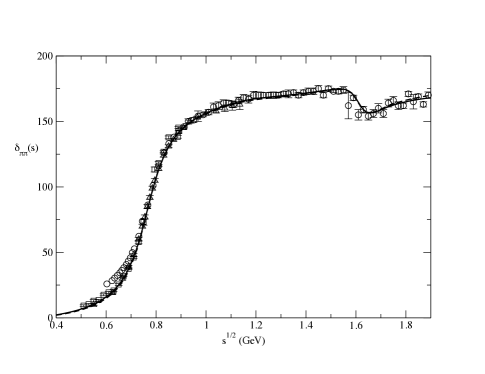
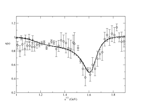
Figure 2: Phase shift (top) and inelasticity (bottom) of the $P$-wave $\pi\pi$ amplitude. Data is taken from Hyams:1973 (circles) ,Protopopescu:1973 (triangles) , and Estabrooks:1974 (squares). The solid line is the result of the fit to $\delta_{\pi}$ and $\eta$ with the analytical $K$-matrix representation described in the text. The dashed line is the result of the extended parametrization described in Section II.4.

If the left hand cut discontinuity of $\hat{t}_{\alpha\beta}(s)$ were known, then the whole amplitude could be reconstructed using the $N/D$ method discussed above and the production vectors $P_{\alpha}(s)$ could be computed from Eq.(16). Unfortunately, to the best of our knowledge, only in the case of $\hat{t}_{\pi\pi}$ is the left hand cut fairly well known Tryon:1974tq . Thus, one needs a model to incorporate the contribution from the $K{\bar{K}}$ channel. One might as well then construct a model that leads to a simple solution of the integral equation in Eq.(16). This is indeed the case if one uses the analytical $K$-matrix representation with the typical choice of the $K$-matrix parametrized in terms of simple poles. Then the singularity of the scattering amplitude for $s<0$ is also given by poles and this in turn allows one to solve Eq.(16) by algebraic methods. We fix the parameters of the $2\times 2$ $K$-matrix so as to reproduce the $P$-wave $\pi\pi$ data from Hyams:1973 ; Protopopescu:1973 ; Estabrooks:1974 (Fig. 2); $\delta_{\pi}$ and $\eta$ are input parameters, and the model will give a prediction for $\delta_{K}$. The $K$-matrix parametrization was already used by Haymes at el. to interpret their data from Hyams:1973 . Unfortunately, instead of using Eq.(14), the unitarity condition employed in Hyams:1973 was

$$Im\hat{t}_{\alpha\beta}(s+i\epsilon)=\sqrt{s}\sum_{\gamma=\pi,K}\hat{t}^{*}_{\alpha\gamma}(s)\hat{\rho}_{\gamma}(s)\theta(s-s_{\gamma})\hat{t}_{\gamma\beta}(s).$$ (26)

This implies

$$Im[\hat{t}^{-1}(s)]_{\alpha\beta}(s)=-(s-s_{\alpha})\sqrt{s-s_{\alpha}}\delta_{\alpha\beta},$$ (27)

and the $K$-matrix representation becomes

$$[\hat{t}^{-1}(s)]_{\alpha\beta}=[K^{-1}(s)]_{\alpha\beta}+\delta_{\alpha\beta}(s-s_{\alpha})\sqrt{s_{\alpha}-s}.$$ (28)

In contrast, the correct unitarity relation in Eq.(14) gives

$$Im[\hat{t}^{-1}(s)]_{\alpha\beta}(s)=-(s-s_{\alpha})\sqrt{\left(1-\frac{s_{\alpha}}{s}\right)}\delta_{\alpha\beta},$$ (29)

which leads to

$$[\hat{t}^{-1}(s)]_{\alpha\beta}=[K^{-1}(s)]_{\alpha\beta}+\delta_{\alpha\beta}(s-s_{\alpha})I_{\alpha}(s),$$ (30)

where

$$I_{\alpha}(s)=I_{\alpha}(0)-\frac{s}{\pi}\int_{s_{\alpha}}^{\infty}ds^{\prime}\sqrt{1-\frac{s_{\alpha}}{s^{\prime}}}\frac{1}{(s^{\prime}-s)s^{\prime}}.$$ (31)

A convenient choice for the subtraction constant, $I_{\alpha}(0)$, is to take $ReI_{\alpha}(M^{2}_{\rho})=0$. Then one of the poles of $K_{\pi\pi}$ corresponds to the Breit-Wigner mass squared, $M^{2}_{\rho}=(0.77\mbox{ GeV})^{2}$, of the $\rho$ meson. Using the general two-pole parametrization of the $K$ matrix,

$$K_{\pi\pi}=\frac{\alpha_{\pi}^{2}}{M_{\rho}^{2}-s}+\frac{\beta_{\pi}^{2}}{s_{2}-s}+\gamma_{\pi\pi},\;K_{KK}=\frac{\beta^{2}_{K}}{s_{2}-s}+\gamma_{KK}$$

$$K_{\pi K}=K_{K\pi}=\frac{\beta_{\pi}\beta_{K}}{s_{2}-s}+\gamma_{\pi K},$$ (32)

where $\alpha_{\pi}^{2}=\Gamma_{\rho}M^{2}_{\rho}/(M_{\rho}^{2}-s_{\pi})^{3/2}$. By fitting the $P$-wave $\pi\pi$ phase shift, $\delta_{\pi}$, and the inelasticity, $\eta$, we find $\Gamma_{\rho}=0.140\mbox{ GeV}$, and

$$\sqrt{s_{2}}=1.4708\mbox{ GeV},\ \ \ \ \beta_{\pi}=0.199,\ \ \ \ \beta_{K}=0.899,$$

$$\gamma_{\pi\pi}=5.62\times 10^{-2},\ \ \ \ \ \gamma_{\pi K}=0.104,\ \ \ \ \ \gamma_{KK}=1.525,$$

with the $\gamma$’s in units of $\mbox{ GeV}^{-2}$. The comparison of the phase shift and the inelasticity obtained with this parametrization with the data is shown in Fig. 2.

Since the $K$ matrix representation of Eq.(30) satisfies all of the properties of the scattering amplitude discussed in Sec.II.2 it is possible to write $t_{\alpha\beta}$ in the ”N/D” representation. We find, choosing to normalize $D_{\alpha\beta}(s)$ at $s_{0}=0$,

$$N_{\pi\pi}(s)=\lambda_{\pi\pi}\frac{s-z_{\pi\pi}}{(s-s_{L,1})(s-s_{L,2})},\;D_{\pi\pi}(s)=\exp\left(-\frac{s}{\pi}\int_{s_{\pi}}ds^{\prime}\frac{\phi_{\pi\pi}(s^{\prime})}{s^{\prime}(s^{\prime}-s)}\right),$$

$$N_{\pi K}(s)=\frac{\lambda_{\pi K}}{(s-s_{L,1})(s-s_{L,2})},\;D_{\pi K}(s)=\frac{s_{1,\pi K}s_{2,\pi K}}{(s-s_{1,\pi K})(s-s_{2,\pi K})}\exp\left(-\frac{s}{\pi}\int_{s_{\pi}}ds^{\prime}\frac{\phi_{\pi K}(s^{\prime})}{s^{\prime}(s^{\prime}-s)}\right),$$

$$N_{KK}(s)=\lambda_{KK}\frac{s-z_{KK}}{(s-s_{L,1})(s-s_{L,2})},\;D_{KK}(s)=\exp\left(-\frac{s}{\pi}\int_{s_{\pi}}ds^{\prime}\frac{\phi_{KK}(s^{\prime})}{s^{\prime}(s^{\prime}-s)}\right),$$

(34)

with $\lambda_{\pi\pi}=5.649$, $\lambda_{KK}=2.271$ and $\lambda_{\pi K}=3.048\mbox{ GeV}^{2}$. Indeed, as discussed above, the left hand cut is reduced to two poles at $s_{L,1}=-13.87\mbox{GeV}^{2}$ and $s_{L,2}=-0.787\mbox{ GeV}^{2}$, respectively. There are also first order zeros in $N_{\alpha\beta}$ at $z_{\pi\pi}=-0.867\mbox{ GeV}^{2}$ and $z_{KK}=-13.78\mbox{GeV}^{2}$. The numerator functions for the elastic amplitudes $\pi\pi$ and $K{\bar{K}}$ are $O(1/s)$, and for the inelastic amplitudes they are super-convergent, i.e. $O(1/s^{2})$. Asymptotically, as shown in Fig. 3, $\phi_{\pi\pi}(s\to\infty)=O(1/\log(s))$ and $\delta_{\pi}$ stays below $180^{0}$, so there is no CDD pole in the $\pi\pi$ channel, which is consistent with the Levinson theorem (cf. Eq.(25)). The same is true for the $K{\bar{K}}$ channel. Above the $K{\bar{K}}$ threshold the phase of the inelastic amplitude $\phi_{\pi K}$ is given by $\phi_{\pi K}=\delta_{\pi}+\delta_{K}$ and from the $K$ matrix we find that asymptotically $\phi_{\pi K}(\infty)=2\pi$, which results in two CDD poles – one at the $\rho$ mass, $s_{1,\pi K}=M_{\rho}^{2}$, and the other at $s_{2,\pi K}=s_{2}+\beta_{\pi}\beta_{K}/\gamma_{\pi K}=3.884\mbox{ GeV}^{2}$.

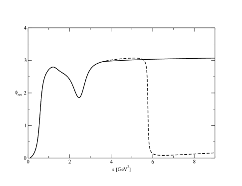
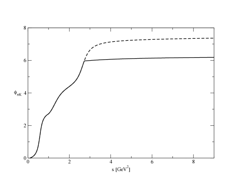
Figure 3: Phase of the $\pi\pi$ (upper) and $\pi K$ (lower) amplitude. The dashed line is the result of the $K$ matrix parametrization from Eq.(34). The solid line is from the modified $K$  matrix parametrization discussed in Sec. II.4

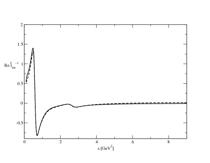
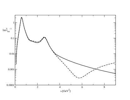
Figure 4: Real (upper) and imaginary (lower) part of $\hat{t}_{\pi\pi}$. The dashed line corresponds to the $K$-matrix solution of E.q 34, and the solid line is the modified $K$-matrix solution, $\hat{t}^{new}_{\pi\pi}$, discussed in Sec. II.4, Eq.(37).

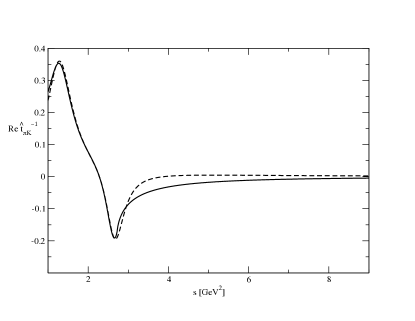
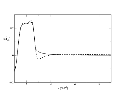
Figure 5: Same as Fig. 4 for $\hat{t}_{\pi K}$ from Eq.(34) (dashed) and $\hat{t}^{new}_{\pi K}$ from Eq.(40).

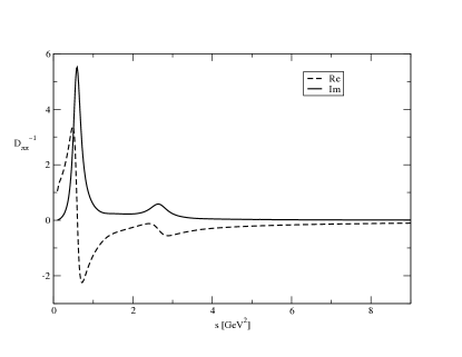
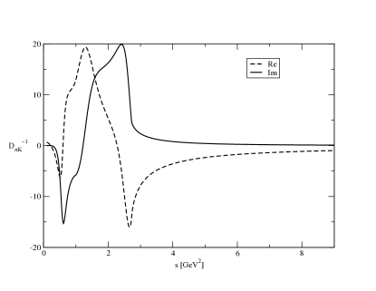
Figure 6: Real (dashed) and imaginary (solid) part of the inverse of $D^{new}_{\pi\pi}(s)$ (upper) and $D^{new}_{\pi K}(s)$ (lower) used in the computation of the isobar form factor, cf. Eq.(44).

Having an analytical representation for the scattering amplitude enables one to identify the resonance content by studying the singularities of $\hat{t}_{\pi\pi}(s)$ for $s$ continued through the unitarity cuts away from the physical sheet. If we define the unphysical sheet II as the one obtained by continuing $s$ from above (crossing) the cut $s_{\pi}<s<s_{K}$, and sheet III for $s$ continued through the $s>s_{K}$ cut, then we find four poles whose location is given in Table 1. The $\rho$ pole is clearly seen as well as the excited $\rho^{\prime}$ resonance at $1600\mbox{ MeV}$ that couples primarily to the $K\bar{K}$ channel. The pole on sheet III at $1.1409-i0.1675$ GeV is most sensitive to the inelasticity of the $K\bar{K}$ channel. If we turn off the $K\bar{K}$ channel this pole goes to infinity while the positions of the other two remain relatively unchanged.

Table 1: Physical poles ($\sqrt{s}$ in GeV) on sheets II and III.

II	III
$0.7638-i0.0747$	$0.7632-i0.0745$
	$1.1409-i0.1675$
	$1.6306-i0.0844$

II.4 Problems with the $K$-matrix parametrization

While the $K$ matrix parametrization faithfully reproduces the $\pi\pi$ phase shift and inelasticity data from $\pi\pi$ threshold up to $1.9\mbox{ GeV}$, extrapolation beyond this range is problematic. The rapid decrease of $\phi_{\pi\pi}$ around $s\sim 6\mbox{ GeV}^{2}$ seems unphysical and results in an absence of the CDD pole at infinity, i.e. $\phi_{\pi\pi}(\infty)\to 0$ instead of $\phi_{\pi\pi}(\infty)\to\pi$ De Troconiz:2001wt . The CDD pole at infinity in the elastic $\pi\pi$ amplitude is expected based on the asymptotic pQCD prediction for the pion electromagnetic form factor Lepage:1980fj . In the $\pi\pi\to K{\bar{K}}$ channel, the two CDD poles at $m_{\rho}^{2}$ and $s_{2}+\beta_{\pi}\beta_{K}/\gamma_{\pi K}$ are clearly an artifact of the pole parametrization of the $K$-matrix. A CDD pole in the inelastic channel above threshold (e.g the pole at $s_{2,\pi K}=3.884\mbox{ GeV}^{2}$) leads to a discontinuity in a phase shift and is unphysical. A pole between $\pi\pi$ and $K{\bar{K}}$ thresholds is admissible, e.g. the pole at $s_{1,\pi K}=m_{\rho}^{2}$, but its strict overlap with the $\rho$ mass is an artifact of the parametrization. Since the phase space available in $J/\psi$ decay extends up to $s_{\pi\pi}\sim 9\mbox{GeV}^{2}$ we need to remove these unphysical features of the $K$-matrix amplitude. We proceed as follows. The new $\pi\pi\to\pi\pi$ and $K{\bar{K}}\to\pi\pi$ amplitudes will be denoted by $\hat{t}^{new}_{\pi\pi}(s)$ and $\hat{t}^{new}_{\pi K}(s)$, respectively. In the case of the $\pi\pi\to\pi\pi$ elastic amplitude, we assume that it has a single CDD pole at infinity. We thus introduce an effective phase shift and inelasticity that asymptotically approach $\pi$ and $1$, respectively:

$$\delta_{eff}(s)=\left\{\begin{array}[]{c}\delta_{\pi}(s),s<s_{K}\\ \pi+(\delta_{\pi}(s_{K})-\pi)\frac{s_{K}}{s},s>s_{K}\end{array},\right.$$ (35)

$$\eta_{eff}(s)=\left\{\begin{array}[]{c}\eta_{\pi}(s),s<s_{K}\\ 1+(\eta_{\pi}(s_{K})-1)\frac{s_{K}}{s},s>s_{K}\end{array}\right.$$ (36)

with $\sqrt{s_{K}}=1.9\mbox{ GeV}$ and $\delta_{\pi}$ and $\eta_{\pi}$ obtained from the $K$-matrix fit below $1.9\mbox{ GeV}$ (cf. Fig. 2). The denominator $D^{new}_{\pi\pi}$ of the effective amplitude

$$\hat{t}^{new}(s)=\frac{N^{new}_{\pi\pi}(s)}{D^{new}_{\pi\pi}(s)}$$ (37)

is then obtained from Eq.(24) with $N_{q}=N_{p}=0$ and phase, $\phi^{eff}_{\pi\pi}$, given by (see Fig. 3)

$$\phi^{new}_{\pi\pi}=\mbox{ Im}\ln\left[\frac{\eta^{eff}e^{2i\delta_{eff}}-1}{2i\hat{\rho}}\right].$$ (38)

For the numerator function $N^{new}_{\pi\pi}$, we use a simple pole approximation to the left hand cut ($s_{L}<0$)

$$N^{new}_{\pi\pi}(s)=\frac{\lambda^{new}_{\pi\pi}}{s-s_{L}}.$$ (39)

In order to remove the unphysical CDD pole from the $K{\bar{K}}\to\pi\pi$ amplitude for $D^{new}_{\pi K}(s)$ in

$$\hat{t}^{new}_{\pi K}(s)=\frac{N^{new}_{\pi K}(s)}{D^{new}_{\pi K}(s)}$$ (40)

for $\phi^{new}_{\pi K}$ in Eq.(24), we use (see Fig. 3)

$$\phi^{new}_{\pi K}=\left\{\begin{array}[]{c}\phi^{K}_{\pi K}(s),s<s_{K}\\ 2\pi+(\phi^{K}_{\pi K}(s)-\pi)\frac{s_{K}}{s},s>s_{K}\end{array}\right.$$ (41)

with $\sqrt{s_{K}}=1.65\mbox{ GeV}$. In this case we use the $K$-matrix fit up to a lower energy of $1.65\mbox{ GeV}$ to be less sensitive to the unwanted CDD pole in the $K$ matrix at $\sqrt{s_{2,\pi K}}=1.97$. There is no effect of this pole in the elastic amplitude, and thus for that case we could use the $K$-matrix parametrization all the way up to $1.9\mbox{ GeV}$ where data exists. Assuming further that $D^{new}_{\pi K}(s)$ has the same asymptotic behavior as $D^{new}_{\pi\pi}$ we add a single CDD pole at $s^{new}_{1,\pi K}$ in place of the pole at $m_{\rho}^{2}$ between the $\pi\pi$ and $K{\bar{K}}$ thresholds. Finally, for the numerator function we use

$$N^{new}_{\pi K}(s)=\frac{\lambda^{new}_{\pi K}}{s-s_{L}}.$$ (42)

i.e we use the same pole to represent the left hand cut as in $N^{new}_{\pi\pi}$. The four parameters $\lambda^{new}_{\pi\pi}$, $\lambda^{new}_{KK}$, $s_{L}$, and $s^{new}_{1,\pi K}$ are determined by simultaneously fitting $\hat{t}^{new}_{\pi\pi}$ and $t^{new}_{\pi\pi}$ to $\pi$ and $K$ phase shifts and inelasticity in the range $2m_{\pi}<\sqrt{s}<1.9\mbox{ GeV}$ and $2m_{K}<\sqrt{s}<1.65\mbox{ GeV}$, respectively. The comparison with the $K$-matrix solution is shown in Figs. 4 and 5 and the fit yields $\lambda^{new}_{\pi\pi}=0.750$, $\lambda^{new}_{\pi K}=0.0477$, $s_{L}=-1.328\mbox{ GeV}^{2}$, and $s^{new}_{1,\pi K}=0.220\mbox{ GeV}^{2}$. As expected, the location of the left hand side pole falls between the two left hand side poles of the $K$-matrix parametrization. In Fig. 6 we show the inverse of the denominator functions $D^{new}_{\pi\pi}$ and $D^{new}_{\pi K}$.

II.5 Interpretation of the $J/\psi\rightarrow 3\pi$ data

With the left hand cut singularities of the scattering amplitudes given by a simple pole, (cf. Eqs.(39),(42)) from Eq.(17) it follows that $ImP_{\alpha}(s)=0$. Thus $P_{\alpha}(s)$ is analytical in the entire $s$-plane and therefore given by a polynomial,

$$P_{\alpha}(s)=(s-s_{L})C_{\alpha}(s).$$ (43)

The first term is responsible for removing the left hand cut singularities from $N^{new}_{\alpha\beta}(s)$ and making $\hat{F}_{\alpha}(s)$ in Eq.(15) analytical for $s<0$. The bound $|P_{\alpha}(\infty)|<1$ restricts $C_{\alpha}(s)$ to be at most a first order polynomial in $s$. Thus the final solution to Eq.(15) has the form

$$F_{1}(s)=Nq_{\pi}(s)p_{\pi}(s)\left[\frac{1+a_{\pi}s}{D^{new}_{\pi\pi}(s)}+r_{\pi K}\frac{1+a_{K}s}{D^{new}_{\pi K}(s)}\right].$$ (44)

The first term corresponds to $J/\psi\to(\pi\pi)_{P}\pi$ and the second to the re-scattering contribution from $J/\psi\to(K{\bar{K}})_{P}\pi\to(\pi\pi)_{P}\pi$.

Figure 7: The isobar form factor $|F_{\pi}(s)|$ with a single $\pi\pi$ channel (dashed) and with both $\pi\pi$ and $K{\bar{K}}$ channels (solid) using the same parameters as in Fig. 10.

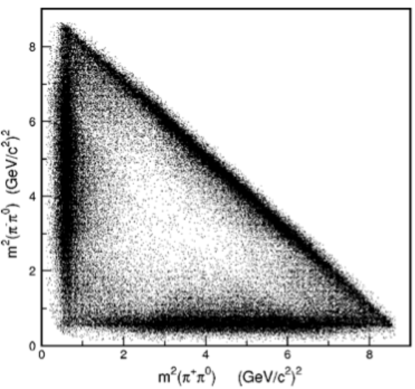
Figure 8: The $J/\psi\to\pi^{+}\pi^{-}\pi^{0}$ Dalitz plot distribution from the BES Collaboration Bai:2004jn .

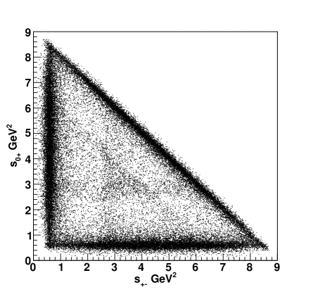
Figure 9: Dalitz plot distribution with the single $\pi\pi$ channel only i.e. $\hat{F}_{1}(s)=q_{\pi}p_{\pi}/D_{11}$ instead of Eq.(44).

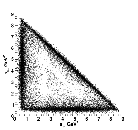
Figure 10: Dalitz plot distribution from $\hat{F}_{1}$ in Eq.(44) with both the $\pi\pi$ and $K\bar{K}$ channels with $a_{\pi}=-1.5\times 10^{-1}\mbox{GeV}^{-2}$ and $r_{\pi/K}=-1.3\times 10^{-2}$.

The Dalitz distribution of $3\pi$ events from $J/\psi$ decays is shown in Fig. 8 and the striking feature is the depletion of events in the center of the plot. This is to be compared with the distribution shown in Fig. 9, which has been generated with $r_{\pi K}=0$. The three bands originate from the $\rho$ meson contribution to $D^{new}_{\pi\pi}$ and the large contribution from the $\rho^{\prime}(1600)$ resonance leads to a significant population of events in the middle of the Dalitz plot that is not seen in the data in Fig. 8. Furthermore in the data there is a large contribution near the tails of the $\rho$ bands, which are absent if only the direct $3\pi$ production is considered. We thus consider the full amplitude from Eq.(44) and float the three parameters $a_{\pi},a_{K}$ and $r_{\pi K}$ to obtain a distribution that best resembles the data. We find little sensitivity to the term proportional to $a_{K}$ and thus set $a_{K}=0$. The parameter $a_{\pi}$ is relevant since it controls the tail of the $\rho$ resonance and so is $r_{\pi K}$ which determines the relative strength of the $K\bar{K}$ contribution which interferes with the $\pi\pi$ amplitude in the $\rho^{\prime}(1600)$ region and reduces the contribution at the center of the Dalitz plot. In Fig. 10 we show the event distribution using $a_{\pi}=-1.5\times 10^{-1}\mbox{GeV}^{-2}$ and $r_{\pi/K}=-1.3\times 10^{-2}$.

The normalization constant $N$ is at this stage arbitrary since we are not determining the absolute value of the branching ratio.

Now, inspecting the Dalitz plot in Fig.10 and the plot of the function $|\hat{F}_{\pi}(s)|$ in Fig.7, it is seen that the $K\bar{K}$ channel can indeed bring theory closer to the data by enhancing the $\pi\pi$ contribution in the energy range $1\mbox{ GeV}<\sqrt{s}<1.5\mbox{ GeV}$ and reducing the strength of the $\rho^{\prime}(1600)$ peak.

III Summary

We have studied the effects of inelastic $\pi\pi$ scattering on the $J/\psi\rightarrow 3\pi$ Dalitz plot. We have seen that the $K\bar{K}\rightarrow\pi\pi$ channel can significantly alter the shape of the Dalitz plot, especially at higher $\pi\pi$ masses. This brings the observed data closer to the phenomenological expectations based on $\pi\pi$ $P$-wave scattering. These coupled channel effects will become even more important as experimental data sets grow larger, for example at BES III, where 1 billion $J/\psi$ decays are expected.

IV ACKNOWLEDGMENTS

This work was supported in part by the US Department of Energy grant under contract DE-FG0287ER40365 and National Science Foundation PIF grant number 0653405.

References

- (1) D. M. Asner et al., arXiv:0809.1869 [hep-ex].
- (2) J. Z. Bai et al. [BES Collaboration], Phys. Rev. D 70, 012005 (2004) [arXiv:hep-ex/0402013].
- (3) B. Aubert et al. [BABAR Collaboration], Phys. Rev. D 70, 072004 (2004) [arXiv:hep-ex/0408078].
- (4) I. J. R. Aitchison and J. J. Brehm, Phys. Rev. D 20, 1119 (1979).
- (5) I. J. R. Aitchison and J. J. Brehm, Phys. Rev. D 20, 1131 (1979).
- (6) I. J. R. Aitchison and J. J. Brehm, Phys. Lett. B 84 (1979) 349.
- (7) R. Kaminski, J. R. Pelaez and F. J. Yndurain, Phys. Rev. D 74, 014001 (2006) [Erratum-ibid. D 74, 079903 (2006)]
- (8) J. J. Brehm, Annals Phys. 108, 454 (1977).
- (9) J.J. Brehm, Phys. Rev. 23, 1194(1981).
- (10) G. Ascoli and H. W. Wyld, Phys. Rev. D 12, 43 (1975).
- (11) N.I. Muskhelishvili, Tr. Tbilis. Math Instrum. 10, 1 (1958); in Singular Integral Equations, J.Radox, ed. (Noordhoff, Groningen, 1985).
- (12) R. Omnés, Nuovo Cim. 8, 316 (1958).
- (13) T. N. Pham and T. N. Truong, Phys. Rev. D 16, 896 (1977).
- (14) G.F. Chew and S. Mandelstam, Phys. Rev. 119, 467 (1960).
- (15) G. Frye and R.L. Warnock, Phys. Rev. 130, 478 (1963).
- (16) L. Castillejo, R.H. Dalitz and F.J. Dyson, Phys. Rev. 101, 453 (1956).
- (17) F. Dyson, Phys. Rev. 106, 157 (1957).
- (18) E. P. Tryon, Phys. Rev. D 12, 759 (1975).
- (19) B. Hyams, C. Jones and P. Weilhammer, Nucl. Phys. B 64, 134(1973).
- (20) S.D. Protopopescu et al. , Phys. Rev. D 7, 1279(1973).
- (21) P. Estabrooks and A. D. Martin, Nucl. Phys. B 79, 301(1974).
- (22) J. F. De Troconiz and F. J. Yndurain, Phys. Rev. D 65, 093001 (2002)
- (23) G. P. Lepage and S. J. Brodsky, Phys. Rev. D 22, 2157 (1980).