EXACT AND QUASI-EXACT MODELS OF STRANGE STARS

Abstract

We construct and compare a variety of simple models for strange stars, namely, hypothetical self-bound objects made of a cold stable version of the quark-gluon plasma. Exact, quasi-exact and numerical models are examined to find the most economical description for these objects. A simple and successful parametrization of them is given in terms of the central density, and many differences among the models are explicitly shown and discussed.

Managing Editor

1 Introduction

We study in this paper a variety of models for strange stars, namely compact objects constituted of an hypothetic cold version of a quark plasma featuring (by hypothesis) a lower energy per baryon than normal hadronic matter. Quarks were suspected to constitute a substantial fraction of a “neutron” star interior since the early ’70s[1][2], and their main properties explored. In 1984[3] the possibility of a star fully composed of quarks up to its surface (but perhaps covered with a “normal” crust) was considered. The simplest model was constructed with a free quark+vacuum energy equation of state (see Ref. jaffe). Because the scale of the strong interactions is set by a multiple of the parameter $B$ of the MIT Bag Model, identified as the vacuum energy density and numerically valued around $60MeV\,fm^{-3}$ or so[5], these compact objects feature masses $\sim 1M_{\odot}$ and radii $\sim 10km$, pretty similar to their “normal” cousins. In fact they may constitute all the “neutron” stars hitherto observed.

The strong interactions (not gravity) bind these kind of compact objects, and at least for the low-mass range $M\leq\,1\,M_{\odot}$, are the responsible for the striking behavior of their mass-radius plot, namely the continuity of models all the way down to pretty small masses $\sim 0.5M_{\odot}$, the minimum allowed by the MIT equation of state. Even though the low-mass stars are clearly newtonian, gravity is increasingly strong at the higher end and forces the use of general relativistic models when $\frac{2GM}{c^{2}R}\geq 0.2$.

As is well-known, the models of these objects can be described, in a first approximation, by the solutions of the Einstein equations for a perfect isotropic, static and spherically symmetric fluid (whose metric is given by $ds^{2}=c^{2}e^{\nu(r)}dt^{2}-e^{\lambda(r)}dr^{2}-r^{2}d\theta^{2}-r^{2}sin^{2}(\theta)d\phi^{2}$):

$$\frac{8\pi G}{c^{2}}\rho(r)=\frac{\lambda^{\prime}e^{-\lambda}}{r}+\frac{1-e^{-\lambda(r)}}{r^{2}},$$ (1)

$$\frac{8\pi G}{c^{4}}p(r)=\frac{\nu^{\prime}e^{-\lambda}}{r}-\frac{1-e^{-\lambda(r)}}{r^{2}},$$ (2)

$$p^{\prime}(r)+\frac{1}{2}(c^{2}\rho(r)+p(r))\nu^{\prime}(r)=0,$$ (3)

where the last equation (contracted Bianchi identity) expresses the conservation of energy-momentum of the fluid.

Mathematically, there are at least three different strategies to solve these equations

• if the pressure, or the density or one metric element is given (for example, by an ansatz), an exact or numerical solution can be found by integration. However, this does not guarantee to have any control over the equation of state $p(\rho)$, and similar solution functions

• instead, if the equation of state $p(\rho)$ is given (i.e. the fluid is characterized from the beginning), the integration can be performed (at least numerically) and the properties of the stellar models follow

• if both the equation of state and one additional function ($p$, $\rho$ or one of the metric) are known, a match of the overdetermined system can be attempted, being in general possible for some values of the involved parameters only.

It is not difficult to envision that the third route can be also employed without an overdetermined system since one provide more degrees of freedom (for example, electric field or pressure anisotropy) at the expense of modifying the originally posed physical problem. We shall return to this point below.

In this work, we have performed three sort of studies:

• the modeling of a strange star by using some of the well known exact solutions (only that ones that meet physical requirements) for the Einstein Field Equation for static and spherically symmetric perfect fluid, e.g., the solutions obtained by the first strategy;

• the modeling of a strange star by the third routine, e.g. overdetermining the system, in order to not only have the microphysics involved (by means of the equation of state), but also to have control over the density profile, chosen to be gaussian as a first reasonable guess;

• a comparison of the above studies to the true solution, or profiles, for a strange star. By true solution, we mean that one obtained closing the system with the equation of state of MIT Bag Model (see below) and numerically integrating the system.

With this we show that the applicability of the well known analytical solutions are rather limited for modeling these stars and the best one can do having in mind the original system is to construct a analytical quasi-exact solution with a overdetermined system, by the expense to introduce an error in the geometry.

Then we show how the introduction of more degrees of freedom (specially pressure anisotropy and the existence of an electric field) can avoid an overdetermined system and at the same provide self-consistent analytical solutions for strange stars.

2 Calculations

2.1 General considerations

As a benchmark for our calculations we have adopted the simplest numerical integration of the massless non-interacting quarks presented, for example, by Alcock, Fahri and Olinto (hereafter AFO) (Ref. afo). This is mainly motivated by the shapes of the profiles obtained by them, which are reproduced in figures 1, 2 and 3. It is clear that any other model in which interactions or finite-quark masses are needed can be obtained analogously (see Ref. jorge for an exploration of the full parameter space of the models).

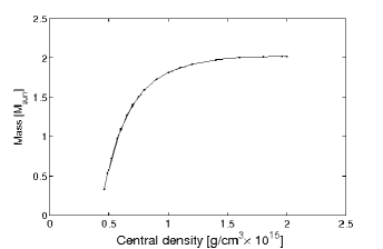
Figure 1: Mass-central density relation of the strange star sequence calculated by Alcock, Farhi and Olinto Ref. 6

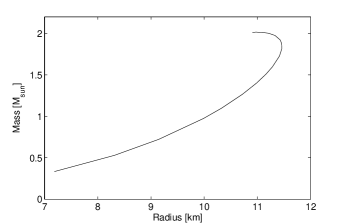
Figure 2: Mass-radius relation of the strange star sequence calculated by Alcock, Farhi and Olinto Ref. 6

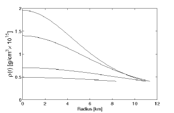
Figure 3: Density profiles of four selected strange stars calculated by Alcock, Farhi and Olinto Ref. 6

Since the main goal of this work is to simplify the description of the stellar models as much as possible, possibly neglecting small ($\leq 1\%$) differences arising from the fact that numerical and exact (or quasi-exact) models do not match exactly, it is useful to parametrize all the features in terms of a single input parameter, chosen to be the central density $\rho_{c}$ which must satisfy $\rho_{c}>4B/c^{2}$ in order to be consistent with the description of the matter in the MIT bag model, where $p=(c^{2}\rho-4B)/3$.

To fix ideas, assume that $f(x)=ag(x)+b$ is a solution of the density profile. If an ansatz is given for $g(x)$, with that profile it is possible to obtain solutions for the pressure and the for the metric elements. Then we fit the parameters $a=a(\rho_{c})$ and $b=b(\rho_{c})$, so that the mass-radius relation of AFO is reproduced as accurately as possible. After this is achieved, we can proceed to derive all the features of any given model.

However, not all exact (or even quasi-exact, see below) solutions describe a viable star: physically acceptable models should fulfil the following conditions, as discussed in the work by Delgaty and Lake (Ref. catalogo_delgaty_lake):

• $e^{\lambda(0)}=1$

  To integrate the Einstein equations, two initial conditions are needed, generally taken as $m(r=0)$ and $p(r=0)$, this is why this condition is so important to define the central region of the star. A small sphere of radius $r=\epsilon$ has a length of $2\pi\epsilon$ and proper radius $e^{\lambda/2}\epsilon$. A small circle around $r=0$ has a ratio of the length to its radius given by $2\pi e^{-\lambda/2}$. However, since the space-time is locally flat, this ratio should be for this small circle around $r=0$, equal to $2\pi$. Thus, $e^{\lambda(0)}=1$ and if $r\rightarrow 0$, then also $m(r)\rightarrow 0$, cf. Ref. schutz;

• $e^{\nu(0)}=constant<1$

  A particle characterized by the geodesic with a given constant $\mathcal{E}$ has an energy $e^{-\nu/2}\mathcal{E}$ relative to a locally inertial observer at rest in this space-time. Since $e^{-\nu/2}=1$ far away from the object, $\mathcal{E}$ is the energy a distant observer would measure if the particle was distant (i.e. the energy at infinity). Since $e^{-\nu/2}>1$ for all other regions not at the infinite, the observer will measure a higher energy than $\mathcal{E}$ in that regions. This extra energy is the energy a particle gains when it falls in the gravitational field of the object. Thus, $e^{-\nu/2}>1\Rightarrow e^{\nu(0)/2}<1$, cf. Ref. schutz;

• $\rho(r)$ regular at the origin and positive definite

  A region around $r=0$, small enough to be called “center of the star” and large enough to maintain the physical features of the fluid at constant (uniform) density, must have a positive value for the fluid to be real;

• $p(r)$ regular at the origin and positive definite

  The pressure at a central core which is approximated by a constant (uniform) density must have a constant positive value, as a result of the properties of real matter;

• $\frac{dp}{d\rho}\leq c^{2}$

  The speed of sound in the fluid should be smaller than the velocity of light.

Our first approach to the problem is described below, using the well-known Tolman IV[10] and Buchdhal I[11], which satisfy all properties 1-5 necessary for realistic models.

2.2 Exact and quasi-exact solutions

2.2.1 Tolman IV and Buchdahl I

Tolman IV and Buchdahl I are two well-known exact solutions featuring mathematically simple expressions for static self-gravitating fluid spheres. Moreover, they are physically sound and fulfil tghe requirements listed in the former section. We have tested the applicability of these simple models to the strange star problem, comparing them with the numerical results of AFO. A previous attempt can be found in Ref. Latt.

We chose these two solutions also because the density profile can be well fitted in order to reproduce the AFO density profile.

Tolman IV

This solution has been found by R. Tolman in his seminal paper (tolman_1939). To solve the Einstein equations, he made an ansatz $e^{\nu}\nu^{{}^{\prime}}/2r=const$, a method that rendered an exact integration of the problem. The functions thus obtained read

$$e^{\lambda}=\frac{1+2r^{2}/A^{2}}{(1-r^{2}/R^{2})(1+r^{2}/A^{2})},$$

$$e^{\nu}=Q^{2}\Big{(}1+\frac{r^{2}}{A^{2}}\Big{)},$$

$$\frac{8\pi G}{c^{2}}\rho(r)=\frac{1}{A^{2}}\frac{1+3A^{2}/R^{2}+3r^{2}/R^{2}}{1+2r^{2}/A^{2}}+\frac{2}{A^{2}}\frac{1-r^{2}/R^{2}}{(1+2r^{2}/A^{2})^{2}}$$

and

$$\frac{8\pi G}{c^{4}}p(r)=\frac{1}{A^{2}}\frac{1-A^{2}/R^{2}-3r^{2}/R^{2}}{1+2r^{2}/A^{2}}.$$

From these expressions, an equation of state, a physical radius (boundary, $r_{b}$) the constant Q and the total mass of the sphere are, respectively

$$\rho(p)=\rho_{c}-5\frac{p_{c}}{c^{2}}+5\frac{p}{c^{2}}+8\frac{(\frac{p_{c}}{c^{2}}-\frac{p}{c^{2}})^{2}}{\frac{p_{c}}{c^{2}}+\rho_{c}},$$

$$r_{b}=\frac{R}{3^{1/2}}\Big{(}1-\frac{A^{2}}{R^{2}}\Big{)}^{1/2},$$

$$Q^{2}=\frac{1-r_{b}^{2}/R^{2}}{1+2r_{b}^{2}/A^{2}},$$

$$M_{bound.cond.}=\frac{c^{2}r_{b}}{2G}\Big{(}1-\frac{(1-r_{b}^{2}/R^{2})(1+r_{b}^{2}/A^{2})}{1+2r_{b}^{2}/A^{2}}\Big{)},$$

with

$$\frac{8\pi G}{c^{2}}\rho_{c}=3\frac{R^{2}+A^{2}}{R^{2}A^{2}},\hskip 28.45274pt\frac{8\pi G}{c^{4}}p_{c}=\frac{R^{2}-A^{2}}{A^{2}R^{2}}$$

with $A$, $R$ and $Q$ three arbitrary constants.

To match numerical strange star models as calculated by AFO with the Tolman IV solution, we seek to reproduce the mass and the radius of each model, that is, to determine $A$, $R$ and $Q$ so that the mass and the radius of the numerical calculations are reproduced. However, the central density could not be adjusted simultaneously (the later depends on $A$ and $R$, which in turn are determined by the radius and mass). A relevant question is whether the resulting equation of state is compatible with the linear expression of the MIT Bag Model. We can easily check that the Tolman IV is not appropriate, first because it is not linear, but more importantly because that it depends on the $A$ and $R$ present in the metric elements. When $A$ and $R$ are adjusted to reproduce accurately the masses and radii of the AFO calculations, they happen to depend on the central density of the model. Therefore, the equation of state varies from model to model (from star to star), in spite that its functional form remains the same. This behavior is illustrated in Fig.4.

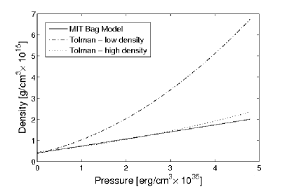
Figure 4: Variation of the equation of state with the constants $A,R$ present in Tolman’s models Ref. 10

It is clear that an equation of state that varies from model to model is not useful to describe a compact star, since the equation of state should reflect the fundamental properties of cold matter and should not behave in this way.

Buchdahl I

Much in the same way as in Tolman IV, we examined the Buchdahl I[11] solution. The expressions are given by

$$e^{\lambda}=\frac{2(1+Cr^{2})}{2-Cr^{2}},$$

$$e^{\nu}=A\big{[}(1+Cr^{2})^{3/2}+B\sqrt{2-Cr^{2}}(5+2Cr^{2})\big{]}^{2},$$

$$\frac{8\pi G}{c^{2}}\rho(r)=-\frac{-\frac{2Cr}{2+2Cr^{2}}-\frac{4Cr(2-Cr^{2})}{(2+2Cr^{2})^{2}}}{r}+\frac{1-\frac{2-Cr^{2}}{2+2Cr^{2}}}{r^{2}},$$

$$\frac{8\pi G}{c^{4}}p(r)=\frac{2\big{[}3Cr\sqrt{1+Cr^{2}}-\frac{BCr(5+2Cr^{2})}{\sqrt{2-Cr^{2}}}+4BCr\sqrt{2-Cr^{2}}\big{]}(2-Cr^{2})}{[(1+Cr^{2})^{3/2}+B\sqrt{2-Cr^{2}}(5+2Cr^{2})](2+2Cr^{2})r}$$

$$\hskip 128.0374pt-\frac{1-\frac{2-Cr^{2}}{2+2Cr^{2}}}{r^{2}},$$

where $A$, $B$ and $C$ are arbitrary constants.

Two types of fits were possible: in the first one we fitted the mass and radius of each model, and as a consequence $\rho_{c}\neq\rho_{c_{AFO}}$ as before. We also attempted to fit both the mass and central density, leading to different radii, depending on the masses. However, we eventually came to the same problem of the non-linearity of the equation of state. Again the obtained equation of state depends on variable quantities and is not useful to model the quark matter.

2.2.2 Quasi-exact gaussian model

An inspection to the density profiles presented by AFO (Figure 3) suggests a simple and popular parametrization of the density dependence. As a simple ansatz we assumed a gaussian profile, a procedure that led to an overdetermination of the system (since the linear MIT equation of state was also imposed). With those assumptions, the following expressions were immediately obtained in closed forms

$$\rho(r)=\Big{(}\rho_{c}-\frac{B}{c^{2}}\Big{)}e^{-r^{2}/r_{o}^{2}}+\frac{B}{c^{2}},$$ (4)

$$p(r)=c^{2}\rho(r)-\frac{4B}{3}$$ (5)

$$\nu(r)=\frac{r^{2}}{2r_{o}^{2}}+a.$$ (6)

$$e^{-\lambda(r)}=\frac{4\pi G\rho_{c}e^{-r^{2}/r_{o}^{2}}r^{2}_{o}}{c^{2}}-\frac{2\pi^{3/2}G\rho_{c}r^{3}_{o}erf(r/r_{o})}{rc^{2}}-\frac{4\pi GBe^{-r^{2}/r_{o}^{2}}r^{2}_{o}}{c^{4}}$$

$$\hskip 71.13188pt+\frac{2\pi^{3/2}GBr^{3}_{o}erf(r/r_{o})}{rc^{4}}-\frac{8\pi Gr^{2}B}{3c^{4}}+1,$$ (7)

$$e^{-\lambda(r)}=\frac{r^{2}_{o}\Big{(}8\pi Gr^{2}e^{-r^{2}/r^{2}_{o}}\rho_{c}c^{2}-8\pi Gr^{2}e^{-r^{2}/r^{2}_{o}}B-24\pi Gr^{2}B+3c^{4}\Big{)}}{3c^{4}(r^{2}+r^{2}_{o})}.$$ (8)

The problem posed in this way reduces to prove whether the two expressions for $\exp(\lambda(r))$, eqs. (7) and (9), are equivalent. Alternatively, even if the functions are different, they could be almost identical inside the star, and therefore a small error would be introduced by employing either one. This is why we speak about quasi-exact solutions for the linear equation of state to stellar problem.

We used as benchmark the same four density profiles shown in AFO for definite values of the total mass $M=1.99$ $M_{\odot}$, $M=1.95$ $M_{\odot}$, $M=1.4$ $M_{\odot}$ and $M=0.53$ $M_{\odot}$.

The idea was to fit expressions for $a$ and for $r_{o}$ (the scale of decay of the density profile) as a function of the central density $\rho_{c}$ which could reproduce the masses and radii.

After that, given any $\rho_{c}$, one may obtain any stellar model along the sequence because he can calculate the total mass, the radius, the metric elements and the density and pressure profiles.

However, it proved impossible to fit all parameters simultaneously without making the system inconsistent. Letting the radius to vary (i.e. relaxing the condition for them to reproduce the AFO results), but keeping the masses and central densities, then the stellar radius $R$, the parameter $a$ and the scale $r_{o}$ could be obtained. As an important remark, we stress that fixing the mass means that the integral of the density function and the boundary condition derived from the metric $\nu(r)$ must be the same, with their values the same as the ones found by AFO.

The fit resulting from just the four profiles did not allow a good determination of $a$ and $r_{o}$. Thus, the grid of models was extended to 20 profiles (i.e. 20 values of the central density) to cover wider mass and radii intervals. The values of $r_{o}$ and $a$ are shown in Table1.

$\rho_{c}[10^{14}g/cm^{3}]$	$M/M_{\odot}[AFO]$	$r_{o}[km]$	$a$
21	2.014042750	7.631010387	-1.780521357
20.5	2.014801608	7.714337813	-1.762999185
20	2.015326779	7.801045927	-1.744982347
19.6	2.015436678	7.872850429	-1.730140677
18	2.013326957	8.185473708	-1.666867564
16	2.002284428	8.646108988	-1.577075908
14	1.975792515	9.212929519	-1.47142208
12	1.921914333	9.936363686	-1.343215145
11	1.877755062	10.38285995	-1.267268177
10	1.815572219	10.90882098	-1.180584905
9	1.726746594	11.54174779	-1.079793495
8	1.597234612	12.32531382	-0.959831395
7.5	1.510155564	12.79466558	-0.890275006
7	1.402444810	13.33296263	-0.81247546
6.5	1.267766569	13.95933096	-0.724422383
6	1.097507111	14.70148514	-0.62334087
5.7	0.973622557	15.21887892	-0.554849121
5.2	0.721604642	16.24225101	-0.423820856
4.885	0.529204878	17.02459731	-0.327483126
4.6	0.333488500	17.85691977	-0.228380811

Table 1: Values of $r_{o}$ and $a$ obtained by imposing the same AFO mass value

Having these values for $a$ and $r_{o}$, we proceeded to derive an accurate functional fit of the form,

$$a(w)=-2.4+9.96e^{(-\frac{w}{0.19})}+2.426e^{(-\frac{w}{0.59})}+1.92e^{(-\frac{w}{3.45})}$$ (9)

$$r_{o}(w)=5.56+22.46e^{(-\frac{w}{0.50})}+10.35e^{(-\frac{w}{2.42})}+169.46e^{(-\frac{w}{0.17})}[km],$$ (10)

where $w\equiv\frac{8\pi G}{c^{2}}l^{2}\rho_{c}$, $l\equiv 10$ $km$, is a dimensionless quantity of the order unity that embodies physical constants ($c$, $G$ etc.) and the lengthscale of the object ($\sim 10km$).

With these values for $r_{o}$ and $a$, we may wonder about the accuracy of the metric element $e^{\lambda(r)}$. We have seen that an ambiguity for this quantity exists. Its first expression was derived from the first Einstein equation (eq. 1) and the second from the second one (eq. 2). How different they really are? Actually it can be checked that the agreement is very good for the lower densities (Figure 5), and worsens for the highest densities (Figure 6) along the stellar sequence. This behavior is a consequence of the newtonian character of the gravitational field for the lower densities, already discussed in Section 1.

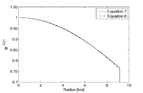
Figure 5: The difference between the two expressions of the metric element $e^{-\lambda(r)}$ inside the star for the model with $\rho_{c}=5.2\times 10^{14}g/cm^{3}$. The radius of the star is marked by the vertical line at the end of the curves. Up: the two expressions; Bottom: the relative error as a function of the radial coordinate.

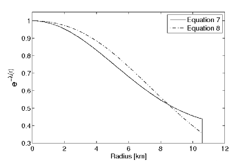
Figure 6: The same as in Fig. 5 for the model with $\rho_{c}=19.6\times 10^{14}g/cm^{3}$. The differences are bigger, as pointed out in the text.

In summary, we have shown that with just the central density value (quite analogously to any other calculation of stellar structure that begins by specifying this value), the values of $a$ and $r_{o}$ can be calculated from the analytical fit. They determine in turn the profiles of density and pressure within the gaussian ansatz, and with them the physical radius of the model $R$. Finally, the mass can be calculated analytically by integrating the gaussian density profile and/or using the boundary condition, yielding the same values within $\lesssim 10\%$ because of the deviations of the fitted expressions from the exact numerical results. We believe that this quasi-analytical model (eqs. 4-8) can be useful for a (very) accurate evaluation of the stellar model structure in a variety of situations.

It is worth to mention at this point that Cheng and Harko[13] presented a very similar approach, starting with the relativistic conditions of thermodynamic equilibrium and the MIT bag equation of state. They found very accurate approximate mass and radius formula for strange stars, in the static case and, amazingly, in the rotating case. Their errors are less than 1% for the former case and 3% for maximally rotating stars.

Considering how the general relativity changes the conditions of thermal equilibrium inside the compact star, they started with the equation for the chemical potential

$$\frac{d\mu}{\mu}=\frac{dp}{\epsilon+p}.$$ (11)

Comparing the conditions at the center and at the boundary (surface)

$$\frac{\mu_{c}^{2}}{\mu_{s}^{2}}=\frac{1}{C(\rho_{c},B)}\Big{(}1-\frac{2GM}{c^{2}R}\Big{)}$$ (12)

and with the MIT Bag equation of the state, they could integrate the equation 11 to obtain

$$\mu=\frac{\mu_{c}}{(\epsilon_{c}-B)^{1/4}}(\epsilon-B)^{1/4}.$$ (13)

Here, the function $C$ is related to the time component of the metric tensor at the center of the star, $g_{00}l_{c}=C(\rho_{c},B)$, that is also related to the redshift of a photon emitted at the center of the star.

Thus, defining the dimensionless parameter $\eta\equiv\rho_{c}/B$, they obtained the following expression to the mass-radius ratio:

$$\frac{M}{R}=\frac{c^{2}}{2G}\Big{[}1-C(\eta)\Big{(}\frac{\eta-1}{3}\Big{)}^{1/2}\Big{]}.$$ (14)

From considerations about the mass continuity on the surface, they proposed the following mass-radius relation

$$M=\frac{16\pi B}{3}a(\eta)R^{3}.$$ (15)

Here, $C(\eta)=const+\sum_{i}a_{i}/\eta^{i}$ ($a_{i}$ constants) and similarly to $a(\eta)$.

Finally, they integrated the Einstein Field Equations numerically and fitted $C(\eta)$ and $a(\eta)$ in order to obtain expressions for the mass and radius in closed forms, where they used $B=56MeV/fm^{3}$.

Their formulae, however, become increasingly inaccurate when $\rho_{c}\rightarrow 4B$.

In the following, we give our derivation for mass and radius, the analogous to their formulae (see eqs. 14 and 15 of Ref. 13),

$$R=\sqrt{-[r_{o}(w)]^{2}ln\Big{(}\frac{3B}{c^{2}\rho_{c}-B}\Big{)}}\hskip 5.69046pt[km]$$ (16)

$$M=5\times 10^{-29}\frac{\Big{(}1-e^{\big{(}\frac{1}{2}\frac{R^{2}}{[r_{o}(w)]^{2}}+a(w)\big{)}}\Big{)}c^{2}R}{2G}\hskip 5.69046pt[M_{\odot}]$$ (17)

We stress two important points about these two expressions. First, they provide the “right” value for the zero-pressure situation, although this feature should not be taken too strictly, because the expressions are only approximations. Second, although they appear quite generic, one should remember that we used $B=57.5MeV/fm^{3}$ to derive $a(w)$ and $r_{o}(w)$. A different value of $B$ would force to recalculate the latter.

The advantage of our approach is that we have the profile for $\rho(r)$, $p(r)$, $\nu(r)$ and $\lambda(r)$ in closed form for each possible value of the central density $\rho_{c}$. Besides that, our formula are in complete agreement with the formula derived by Cheng and Harko[13].

We also point out that recently, Narain, Schaffner-Bielich and Mishustin[14] have made a numerical calculation integrating the dimensionless TOV equation with a linear equation of state for generic fermionic matter. The possibility of scaling the solutions of the TOV problem was already known and exploited, for example, in Witten’s paper [3]. Using this property, Narain, Schaffner-Bielich and Mishustin found a very useful general scaling solution and discussed how to rescale these equations in order to find the solutions for arbitrary fermion masses and interacting strengths. In spite of this generality, we point out that our process of making the equations dimensionless is different from that work and, moreover, the choice of a gaussian form induces the presence of the length $r_{o}$ which controls the spatial decay of the density. As a result, it is not possible to compare easily our quasi-exact models with their results, which remain more general but require the knowledge of the dimensionless $M-R$ curve.

2.2.3 Polytropic models

A recent interesting approach has been presented by Lai and Xu[15], which models a quark star with a polytropic equation of state. This kind of equation of state is generally stiffer than that conventional linear one, like the bag model. Unfortunately, exact solutions are difficult to obtain for the polytropic case. However, their numerical results are interesting because they deal with two models: with and without QCD vacuum energy ($\Lambda$), and show how they compare to linear bag-like equations of state. See their numerical results in Figure 2 from Ref. xu.

As a general feature we may say that the work of Lai and Xu shows that a polytropic description of strange stars is possible and accurate, but it does not provide an easy and economical form for generating models, at least not easier than a full numerical work.

2.2.4 Exact anisotropic model

The exact anisotropic model of Sharma and Maharaj[16] is another accurate approximation for the stellar structure and needs, as above, just one parameter (the central density). As a physical motivation to consider this anisotropy, they quote Usov[17] that suppose a strong electric field formed into a thin layer at the quark surface of a bare strange star. This is possible due the depletion of s-quarks in this region.

The exact expressions of this models are

$$\rho(r)=\frac{b(3+ar^{2})}{8\pi(1+ar^{2})^{2}},$$ (18)

$$m(r)=\frac{r^{3}b}{2(1+ar^{2})},$$ (19)

$$p_{r}(r)=\frac{c^{2}b(3+ar^{2})}{24\pi(1+ar^{2})^{2}}-\frac{4B}{3},$$ (20)

$$e^{\lambda(r)}=\frac{(1+ar^{2})c^{2}}{(c^{2}a-Gb)r^{2}+c^{2}},$$ (21)

$$e^{\nu(r)}=e^{Xr^{2}}(1+ar^{2})^{1/3}(c^{2}+c^{2}ar^{2}-Gr^{2}b)^{Y}K$$ (22)

$$p_{t}(r)=p_{r}(r)-\frac{1}{2}\Bigg{[}-\frac{c^{2}bar}{12\pi(1+ar^{2})^{2}}+\frac{c^{2}bar(3+ar^{2})}{6\pi(1+ar^{2})^{3}}$$

$$\hskip 71.13188pt-\frac{(\frac{c^{2}b(3+ar^{2})}{12\pi(1+ar^{2})^{2}}+\frac{4B}{3})(\frac{Gr^{3}b}{2(1+ar^{2})}+\frac{4\pi Gr^{3}p_{r}(r)}{c^{2}})}{r(c^{2}r-\frac{Gr^{3}b}{1+ar^{2}})}\Bigg{]}r$$ (23)

and are enough to obtain the mass-radius relation, the density profile, and the pressures (tangential and radial). Here, $b=8\pi\rho_{c}/3$ and $a=1/r_{o}^{2}$. We have checked that the anisotropy is small (see Figure 7) in the interval of central densities. Once the free parameters $r_{o}$ and $K$ are fitted as functions of the central density $\rho_{c}$ the models are completely specified. We show the resulting mass-radius relation in Figure 8.

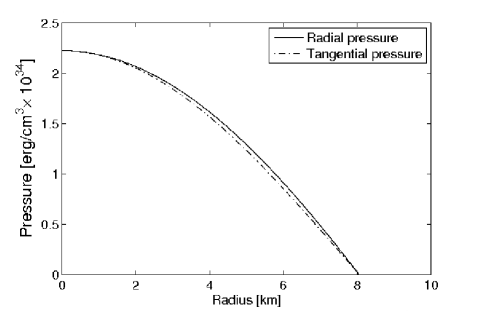
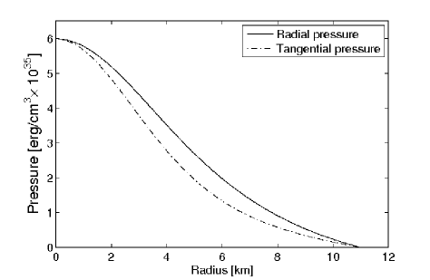
Figure 7: Radial and tangential pressures for two anisotropic stellar models. Up: $\rho_{c}=4.8\times 10^{14}g/cm^{3}$; Bottom: $\rho_{c}=24\times 10^{14}g/cm^{3}$.

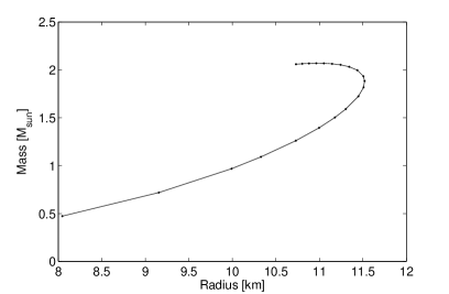
Figure 8: Mass-radius curve for the anisotropic model of Sharma-Maharaj Ref. 16

The similarity of the curve in Figure 8 and the numerical results by AFO is apparent. However, in spite that masses and radii are practically the same, anisotropic models are systematically denser at the center by $25\%$ or so. For example, the maximum mass model along the sequence has a central density of $\simeq 24\times 10^{14}g/cm^{3}$ whereas in the AFO numerical calculation the value is just $\simeq 20\times 10^{14}g/cm^{3}$. The density profiles are shown in Figure 9. It is also apparent the similarities with AFO.

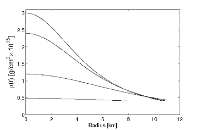
Figure 9: Density profiles of the anisotropic models of Sharma-Maharaj Ref. 16

Ruderman[18] argued that the anisotropies could be important for densities $\rho>10^{15}g/cm^{3}$. This is consistent with our results. It should be pointed out, however, that the anisotropy could affect some parameters like the maximum mass (the effect is small in our approach) and the redshift, as discussed long ago by Bowers and Liang[19].

Only the analytical solution for the anisotropic star is not sufficient for a complete description of such an object. This is because it is important to explain where the anisotropy comes from in order to produce the differences we have shown. Mak and Harko[20] pointed out that a source of anisotropy could be an anisotropic velocity distribution of the particles inside the star due, for example, a magnetic field, turbulence or convection. Perhaps the biggest challenge of the anisotropic model is the stability criterion. Chan et al[21] showed that, in the onset of instabilities, even small anisotropies might drastically change the stability of the system.

We have shown that the pressure anisotropy is small for low central densities but becomes larger and larger as the central density increases. Further studies are necessary in our approach to verify if all the sequence (e.g. in all central density range) is stable.

2.2.5 Exact electric field model

In the same way as before, we explored the model developed by Komathiraj and Maharaj[22] to model strange stars parametrized by a single parameter, the central density. This model also has all the desirable properties cited above. However, the electric field is an explicit function of the position coordinate, starting from zero at the center and growing up to the surface. The effect of this field on the mass-radius relation is to increase the masses and respective radii. The mass-radius relation is shown in Figure 10.

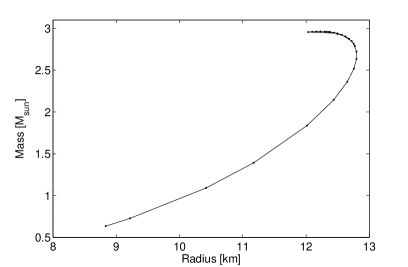
Figure 10: Mass-radius curve for the electric model of Komathiraj-Maharaj Ref. 22

In this model, we deal with a charged strange star. It is important to notice that this is quite different from the assumption made by Usov, since the charge is distributed inside the whole star. Charged compact stars also have been studied in many ways by Ray et al.[23]. In this work they have found that a star can have a electric field about $\sim 10^{21}V/m$ in a particular case of polytropic equation of state. It is interesting to notice that the Komathiraj-Maharaj exact solution with electric field also provides electric fields at boundary $>1.5\times 10^{20}V/m$.

3 Conclusions

We have used a wide set of mathematical solutions (exact and approximate) in order to model strange quark stars. All these solutions were parametrized by a single quantity, the central density. Both simple exact and quasi-exact models were addressed, with and without extra degrees of freedom (anisotropy and electric field).

No simple analytical model was found to describe these stars by keeping the equation of state functionally unchanged (see 2.2.1). Solutions other than the ones discussed here should be examined having this description in mind.

In our particular treatment, the quasi-exact solution, we have used a grid with 20 points, corresponding to 20 central densities and we have fitted expressions for the free parameters of the problem that solves analytically the Einstein equations for a perfect fluid with spherical symmetry and a linear equation of state. The success of this particular approach can be gauged in Figure 11, that summarizes the mass-radius relations of all solutions found and also in Figure 12 where we show the density profiles of the stars of maximum mass from some solutions (Tolman, Buchdahl, gaussian-approximated and anisotropic). We remind that this work used the simple numerical models of AFO as a benchmark, but the later has a small number of degrees of freedom, being based on the MIT bag equation of state. This linear behavior, however, makes the fluid equation system impossible to be integrated analytically unless we give an extra equation overdetermining the system. If this is done, then it is necessary a match of the overdetermined system.

We have shown that it is possible to find a quasi-exact solution that is useful to model a strange star in an easy way. We just give the central density and all other quantities like de mass, radius, profiles etc. can be found. With these analytical expressions we can predict many properties of the star defined by that central density. The errors remain $\leq 1\%$ in all quantities, including the geometry (Fig. 5 and 6).

We can see in the Figure 11 that the gaussian-approximated solution is valid in the range of low central densities, matching almost exactly to AFO. The anisotropic model is valid for all range of central densities and is not very different of AFO. This is a promising model (see Figure 9 and compare it with Figure 3; but see also the remarks in the section 2.2.4). The electric field model is also valid, but only in the context of charged quark stars.

This integrability problem does not happen with a system of fluid equations featuring anisotropic pressure or an electric field. These new degrees of freedom makes the system integrable. We have discussed how these results compare to the linear, isotropic, uncharged models and how they affect the actual stellar features in practice.

It should be reminded that, in spite of their deep physical differences, it is too early to dismiss any equation of state for strange stars. The extraction of the radius from the observation of thermal-like emission is still problematic and may contain substantial inaccuracies. Taken at face value, however, the determinations have rendered small numbers, certainly incompatible with neutron star models if true. For example, the objects EXO 0748-676[24] [$2.10\pm 0.28M_{\odot},\geq 13.8\pm 1.8km$] and EXO 1745-248[25] [$1.4M_{\odot},11km$] or [$1.7M_{\odot},9km$] can be described by the anisotropic model (taking into account the error bars) respectively [$2.0M_{\odot},11.44km$] and [$1.39M_{\odot},11.0km$] (this last one with a claimed high precision). We conclude this work pointing out that simple, economical descriptions of a variety of strange stars can be constructed and may be useful to explore their properties and structural behavior in many static and dynamical situations.

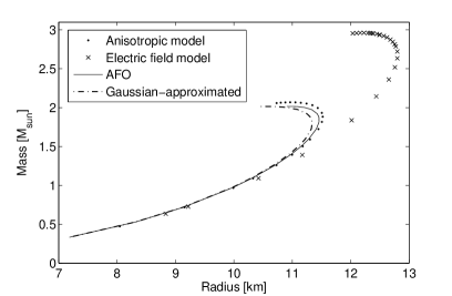
Figure 11: Mass-radius relations for various models.

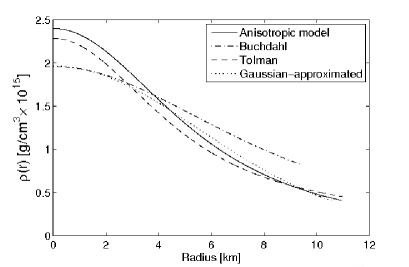
Figure 12: Density profiles of the stars of maximum mass.

References

- [1] N. Itoh, Progress of Theoretical Physics 44 (1970) 291.
- [2] J. C. Collins and M. J. Perry, Physical Review Letters 34 (1975) 1353.
- [3] E. Witten, Phys. Rev. D 30 (1984) 272.
- [4] T. Degrand and R. L. Jaffe and K. Johnson and J. Kiskis, Phys. Rev. D 12 (1975) 2060.
- [5] F. Weber, Pulsars as astrophysical laboratories for nuclear and particle physics, 1st edn. (Institute of Physics Publishing, Bristol and Philadelphia, 1999).
- [6] C. Alcock and E. Farhi and A. Olinto, Astrophys. Jour. 310 (1986) 261.
- [7] O. G. Benvenuto and J. E. Horvath, Monthly Notices of the R.A.S. 241 (1989) 43.
- [8] M. S. R. Delgaty and K. Lake, Computer Physics Communications 115 (1998) 395.
- [9] B. F. Schutz, A First Course in General Relativity, 1st edn. (Cambridge University Press, Cambridge UK, 1985).
- [10] R. C. Tolman, Phys. Rev. 55 (1939) 364.
- [11] H. A. Buchdahl, Phys. Rev. 116 (1959) 1027.
- [12] J. M. Lattimer and M. Prakash, Phys. Rev. Lett. 94 (2005) 111101.
- [13] K. S. Cheng and T. Harko, Phys. Rev. D 62 (2000) 083001.
- [14] G. Narain, J. Schaffner-Bielich and I. Mishustin, Phys. Rev. D 74 (2006) 063003.
- [15] X. Y. Lai and R. X. Xu, Astroparticle Physics 31 (2009) 128.
- [16] R. Sharma and S. D. Maharaj, Monthly Notices of the R.A.S. 375 (2007) 1265.
- [17] V. V. Usov, Phys. Rev. D 70 (2004) 067301.
- [18] Ruderman, R., A. Rev. Astr. Astrophys. 10 (1972) 427.
- [19] Bowers, R. L. and Liang, E. P. T., Astrophys. J. 188 (1974) 657.
- [20] M. K. Mak and T. Harko, Proc. R. Soc. Lond. A 459 (2003) 393.
- [21] Chan, R., Herrera, L. and Santos, N. O., Monthly Notices of the R.A.S. 265 (1993) 533.
- [22] K. Komathiraj and S. D. Maharaj, ArXiv e-prints:astro-ph/0712.1278 712 (2007).
- [23] S. Ray, M. Malheiro, J. P. S. Lemos and V. T. Zanchin, Braz. Jour. Phys.34(2004) 310 ; see also Proceedings of the MG10 Meeting, Rio de Janeiro, Brazil, 20-26 July 2003, Eds.: Mario Novello; Santiago Pérez Bergliaffa and Remo Ruffini (World Scientific, Singapore, 2005) p.1361.
- [24] F. Ozel, Nature 441 (2006) 1115.
- [25] F. Ozel, T. Guver and D. Psaltis, ArXiv e-prints:astro-ph/0810.1521 810 (2008).