Decentralized Fair Scheduling in Two-Hop Relay-Assisted Cognitive OFDMA Systems

Abstract

In this paper, we consider a two-hop relay-assisted cognitive downlink OFDMA system (named as secondary system) dynamically accessing a spectrum licensed to a primary network, thereby improving the efficiency of spectrum usage. A cluster-based relay-assisted architecture is proposed for the secondary system, where relay stations are employed for minimizing the interference to the users in the primary network and achieving fairness for cell-edge users. Based on this architecture, an asymptotically optimal solution is derived for jointly controlling data rates, transmission power, and subchannel allocation to optimize the average weighted sum goodput where the proportional fair scheduling (PFS) is included as a special case. This solution supports decentralized implementation, requires small communication overhead, and is robust against imperfect channel state information at the transmitter (CSIT) and sensing measurement. The proposed solution achieves significant throughput gains and better user-fairness compared with the existing designs. Finally, we derived a simple and asymptotically optimal scheduling solution as well as the associated closed-form performance under the proportional fair scheduling for a large number of users. The system throughput is shown to be $\mathcal{O}\left(N(1-q_{p})(1-q_{p}^{N})\ln\ln K_{c}\right)$, where $K_{c}$ is the number of users in one cluster, $N$ is the number of subchannels and $q_{p}$ is the active probability of primary users.

EDICS Items: WIN-CLRD, WIN-CONT.

I Introduction

Dynamic spectrum access [1] is a new paradigm to meet the challenge of the rapidly growing demands of broadband access and the spectrum scarcity for designing the next-generation wireless communication systems. This motivates the study in this paper on designing a two-hop relay-assisted cognitive OFDMA system which dynamically shares spectrum access with a primary system (PU) by exploiting its idle periods.

I-A Related Work and Motivation

The issues of power control for dynamic spectrum access in ad hoc networks are addressed in [2, 3, 4]. Cellular systems using cognitive radio for dynamically accessing the television spectrum are being standardized by the IEEE 802.22 working group. In [5], a joint beamforming and power control algorithm is proposed for a cognitive cellular systems to mitigate interference to the primary network. A key obstacle for implementing dynamic spectrum access in cellular systems is that direct transmission from base stations to cell-edge users requires large power and thus causes strong interference to the users in the primary networks. As a result, the users in the cell-edge will have very small access opportunity due to the primary user activities and this fairness issue cannot be solved by simply fair scheduling at the base station because the users on the cell edge is limited by the channel access opportunity rather than the scheduling opportunity. Hence, relay-assisted cellular system will be an effective solution for alleviating the above fairness issue because it helps to reduce the transmission power required to reach the mobiles on the cell edge. However, there are still a few critical issues associated with the design and operation of relay-assisted CR systems as summarized below.

• Optimal Decentralized Power, Rate and Subchannel Allocation Algorithm: Extensive research has been carried out on resource allocation in point-to-point relay-assisted communication systems. Power and subchannel allocations for relay-assisted OFDMA systems are studied in [6, 7, 8, 9, 10, 11, 12, 13, 14, 15, 16]. However, these existing works consider centralized solution (e.g. at BS) in which the resource (power, rate and subchannel) allocation of the BS and the RSs is computed in a centralized manner at the BS based on the global system state knowledge . Hence, the conventional centralized approach is very difficult to implement in practice due to huge signaling overhead and computational complexity. Moreover, various simplifying assumptions were made in these literatures to simplify the resource allocation problem in 2-hop OFDMA systems at the cost of performance loss. For example, one typical constraint is that the relay can only receive the data for one MS in each subchannel, and this data should be forwarded completely and exclusively to the target MS in one subchannel in next phase [10, 12]. This may cause significant performance loss when the BS-RS link is much better than the RS-MS link. Therefore, the challenge is to have a decentralized solution without performance loss compared with the centralized solutions.

• Fairness Consideration in Two Hop Systems: Conventional relay-assisted cellular systems perform resource allocation to maximize the sum-throughput [6, 7]. Yet, fairness is an important requirement and a general solution of fair scheduling in relay-assisted (two-hop) CR system is still not fully addressed. When fairness is considered in a relay-assisted system, neither the optimization objective nor the flow balance constraint for the relays is convex. Therefore, the conventional approaches for the sum-throughput optimization in the previous works cannot be applied, and how to solve such resource allocation problem with fairness consideration in relay-assisted systems is an important challenge to overcome.

• Dynamic Spectrum Access with Imperfect CSIT and Sensing Measurement: In conventional resource optimization problems in relay-assisted systems [6, 7], there is no consideration on dynamic spectrum sharing aspects. However, the presence of PU activity and dynamic spectrum sharing has changed the fundamental dynamics of the resource allocation problem. For efficient spectrum sharing, it is critical for the CR systems to be able to exploit the temporal and spatial burstiness of the PU activity gaps and yet at the same time, without interrupting the PU transmissions. This problem is even more challenging when we have to take into account the imperfect channel state information and sensing measurement in which interference to the PU cannot be completely avoided.

I-B Contributions

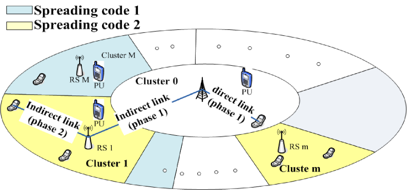
Figure 1: Cluster based relay-assisted downlink OFDMA system.

The key contributions of our work are summarized as follows. We consider a cluster-based two-hop RS-assisted cognitive OFDMA system, as shown in Figure 1 and 2. We are interested in the associated resource control problem, which is a difficult non-convex problem. Moreover, traditional centralized optimization approach requires significant communication overhead between the base station and the relay stations, and has exponentially many control variables w.r.t. the number of independent subchannels. In order to tackle these difficulties, we divide and conquer the resource control problem into a base station master problem and the relay station subproblems, where the number of control variables is significantly reduced (grows linearly w.r.t. the number of frequency bands). We derive a low-complexity, low-overhead and decentralized algorithm for controlling power, rate, and subchannel allocation, which asymptotically maximizes the weighted sum goodput (average b/s/Hz successfully received by the MS) under the primary-user interference constraint. We also include the well-known proportional fair scheduling (PFS) as a special case in our formulation. The solution accounts for multiuser diversity, user fairness, imperfect channel state information at the transmitter (CSIT) and spectrum sensing. As shown by simulations, the proposed resource allocation algorithm significantly improves the fairness for cell-edge users. Finally, a simple and asymptotically optimal scheduling policy as well as the closed-form performance for PFS is derived to obtain design insights. For instance, we show that the throughput of the proposed two-hop relay-assisted cognitive OFDMA system under PFS is $\mathcal{O}\left(N(1-q_{p})(1-q_{p}^{N})\ln\ln K_{c}\right)$, where $K_{c}$ is the number of users in one cluster, $N$ is the number of independent subchannels and $q_{p}$ is the active probability of primary users on one subchannel.

The remainder of this paper is organized as follows. The system model is described in Section II. In Section III, the problem of optimal power, rate, and subchannel allocation is formulated; the solutions are presented in Section IV. Asymptotic throughput analysis is given in Section V. Section VI contains simulation results, followed by concluding remarks in Section VII.

II System Model

II-A Architecture and Protocol

As illustrated in Figure 1, the secondary user (SU) system is a cluster-based relay-assisted cognitive OFDMA downlink system consists of one base station (BS) transmitting to $K$ mobile users (MS), where communications are assisted by $M$ relay stations (RS) as elaborated shortly. The cell is divided into $M+1$ clusters as shown in Figure 1. The central cluster (served by the BS) is indexed as the $0$-th cluster, whose users directly communicate with the base station over relatively short distances. Each of the remaining $M$ clusters is served by a half-duplexing RS. Specifically, each RS forwards data packets from the base station to users in the its cluster using the decode-and-forward (DaF) strategy. The number of users in the $m$-th cluster is denoted as $K_{m}$. For the notation convenience, we assume that the first $M$ users in the $0$-th cluster are the $M$ RSs, and the remaining $K_{0}-M$ users in the $0$-th cluster are the MSs of the $0$-th cluster ($K_{0}+K_{1}+...+K_{M}=K+M$).

The above secondary user (SU) system is assumed to opportunistically access a spectrum licensed to another network, whose users are referred to as the primary users (PU) and have the highest priority of using the spectrum. Primary users are distributed over the service area of the SU system. To avoid interrupting the communication of primary users, every transmitter (including the BS and the RSs) of the SU system is not allowed to transmit if there is active PU in the coverage.

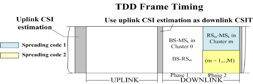
Figure 2: A frame structure example for relay-assisted OFDMA system.

The protocol for relay transmission is described as follows. The channels are assumed to be frequency selective and divided into $N$ independent subchannels using the orthogonal frequency division multiplexing (OFDM) modulation [17]. Downlink transmission is divided into frames, each with two phases (as illustrated in Figure 2). In phase one, the base station delivers packets to the MSs of the $0$-th cluster and all the RSs; in phase two, each RS forwards data packets to the MSs in the corresponding cluster. To avoid interfering MSs in other clusters, we have the following assumption:

Assumption 1

The base station does not deliver packets in phase two. In order to control the inter-cluster interference between two adjacent relay clusters, the transmitted signals at the adjacent RSs are spread by different orthogonal spreading sequences in the frequency domain as illustrated in Figure 1.

II-B Channel Model

The channel realization is assumed to be quasi-static over one frame but independent and identically distributed (i.i.d.) across different frames. Channel gains are characterized by the long-term path loss, shadowing and the short-term fading. The symbol received at the $k$-th user of the $m$-th cluster in the $n$-th subchannel, denoted as $Y_{m,n,k}$, can be written as

$$Y_{m,n,k}=\sqrt{p_{m,n,k}l_{m,k}}H_{m,n,k}X_{m,n,k}+Z_{m,n,k},$$

where $X_{m,n,k}$ is the transmitted symbol, $p_{m,n,k}$ is the transmission power, $l_{m,k}$ is the long-term channel attenuation due to path loss and shadowing, $H_{m,n,k}\sim\mathcal{CN}(0,1)$ models short-term fading, and $Z_{m,n,k}\sim\mathcal{CN}(0,1)$ represents the additive white Gaussian noise. Note that $H_{m,n,k}$ represents the channel between the $k$-th user and the base station if $m=0$, or the $m$-th relay station if $m>0$.

The BS and RSs adapt the data rates, power, subchannel allocation for the downlink transmission based on the CSI at the transmitter (CSIT). We consider a time division duplex (TDD) system where the CSIT can be acquired by channel reciprocal [18]. Due to CSI estimation noise as well as duplexing delay, the CSIT obtained will not be accurate and the CSIT error model (based on MMSE prediction) is given by [18]:

$$\hat{H}_{m,n,k}=H_{m,n,k}+\Delta H_{m,n,k},\quad\forall m,n,k$$ (1)

where $H_{m,n,k}$ represents actual CSI, $\Delta H_{m,n,k}$ represents the CSIT error which is modelled as complex Gaussian distribution with mean 0 and variance $\sigma^{2}_{e}$ ($\Delta H_{m,n,k}\sim\mathcal{CN}(0,\sigma^{2}_{e})$), and $\mathbf{E}[\Delta H_{m,n,k}\hat{H}_{m,n,k}]=0$ (meaning that the estimation error $\Delta H_{m,n,k}$ is uncorrelated to CSIT $\hat{H}_{m,n,k}$). For convenience, the CSIT is grouped according to cluster as the sets $\mathbf{\hat{H}}_{m}=\cup_{n,k}\{\hat{H}_{m,n,k}\}$ for $0\leq m\leq M$, which are referred to as local CSIT at the $m$-th cluster. The set $\mathbf{\hat{H}}=\bigcup\limits_{m=0}^{M}\mathbf{\hat{H}}_{m}$ is called as global CSIT.

II-C Dynamic Spectrum Access and Fairness Issues

In each cluster, each secondary user senses the spectrum and searches for subchannels unused by primary users, which, for instance, may be wireless microphones or other Part 74 devices [19]. The spectrum sensing results consist of binary indicators specifying the availability of subchannels. These sensing resutls are referred to as raw sensing information (RSI) in this paper. Let $\hat{S}_{m,n,k}\in\{0,1\}$ denote the sensed state at the $k$-th user on the $n$-th subchannel in the $m$-th cluster, where $\hat{S}_{m,n,k}=1$ and $0$ correspond to the states “available” and “unavailable”, respectively. RSI $\hat{\mathbf{S}}_{m}=\{\hat{S}_{m,n,k}|\forall n,k\}$ is communicated by users to their corresponding servers (BS/RS) for enabling resource allocation. Moreover, we also define the aggregation of RSI from all clusters as $\hat{\mathbf{S}}=\{\hat{\mathbf{S}}_{m}|\forall m\}$. Let $S_{m,n}$ be the actual primary-user state on the $n$-th subchannel in the $m$-th cluster with $S_{m,n}=1$ denoting subchannel is actually available and $S_{m,n}=0$ denoting otherwise, $\mathbf{S}_{m}=\{S_{m,n}|\forall n\}$ be the actual PU activity of all the subchannels in the $m$-th cluster and $\mathbf{S}=\{\mathbf{S}_{m}|\forall m\}$ be the aggregation of actual PU activity of all clusters which is quasi-static over a number of frames. Moreover, define $q_{p}=\Pr(S_{m,n}=1)$ as the probability one subchannel is available, which is assumed to be identical for all $m$ and $n$. In practice, we cannot have perfect sensing at the mobile and there exist nonzero probabilities for the events false alarm $\left(q_{f}=Pr(\hat{S}_{m,n,k}=0|S_{m,n}=1)\right)$ and mis-detection $\left(q_{m}=Pr(\hat{S}_{m,n,k}=1|S_{m,n}=0)\right)$ [20]. Moreover, $q_{d}=1-q_{m}$ represents the probability of detection.

Due to the imperfect sensing measurement, it is not possible to eliminate the interference from the SU to the PU systems. To protect communication in the PU networks, we require

$$I_{m,n}=(\sum_{k=1}^{K_{m}}p_{m,n,k})\tau_{m,n}(1-\mathbf{E}[S_{m,n}|\widehat{\bf S}_{m,n}])\leq\overline{I},\quad\forall m,n,$$ (2)

where $I_{m,n}$ is the conditional average interference level (conditioned on the sensing measurement) from the SU (at the $m$-th cluster and the $n$-th subchannel) to the active PU, $\widehat{\bf S}_{m,n}=\{{\hat{S}}_{m,n,k}|k\in\{1,K_{m}\}\}$, $p_{m,n,k}$ is the transmit power of the $m$-th RS (or BS) to its $k$-th MS in the $n$-th subchannel, $\tau_{m,n}$ is the path loss between the SU transmitter (at the $m$-th cluster and the $n$-th subchannel) and the active PU. Thus, each SU transmitter should guarantee that the average interference to the active PU in its cluster area is not larger than one tolerance threshold $\overline{I}$.

Remarks (Fairness Issue with Cognitive OFDMA Systems without RS): Consider a simple scenario where we have one PU in each of the M RS clusters as well as the BS cluster as shown in Figure 1. As a result, there are $M+1$ PUs in the system. Let $q_{p}$ be the probability that the PU in a cluster becomes active in one subchannel. If there are no RS in the SU system in Figure 1, the access opportunity of a cell-edge user (users in the cluster $m>0$) in one subchannel is $(1-q_{p})^{M+1}$, which is the probability for all the $M+1$ PUs in the BS’s coverage area to be idle. Hence, the cell-edge users could hardly access the spectrum even for moderate PU activity, leading to critical fairness issue.

III Joint Control of Rate, Power and Subchannel Allocation: Problem Formulation

In this section, we shall formulate the rate, power and subchannel allocation design as an optimization problem. We first formally define the optimization variables (control policies) as well as the optimization objectives below.

III-A Definitions of Control Policies

Consider transmitting to the $k$-th user in the $0$-th cluster (the BS’s cluster) over the $n$-th subchannel. The transmission power, rate and percentage of subchannels the base station allocates to the user is denoted as $p_{0,n,k}(\hat{\mathbf{H}},\hat{\mathbf{S}})$, $r_{0,n,k}(\hat{\mathbf{H}},\hat{\mathbf{S}})$ and $\alpha_{0,n,k}(\hat{\mathbf{H}},\hat{\mathbf{S}})$ respectively, which are adapted to the imperfect CSIT $\hat{\mathbf{H}}$ and RSI $\hat{\mathbf{S}}$. The corresponding polices for controlling transmit power ($\mathcal{P}_{0}$), subchannel allocation ($\mathcal{A}_{0}$) and transmit data rate ($\mathcal{R}_{0}$) are defined as the function sets $\mathcal{P}_{0}:=\left\{p_{0,n,k}(\hat{\mathbf{H}},\hat{\mathbf{S}})|\forall n,k\right\}$, $\mathcal{A}_{0}=\left\{\alpha_{0,n,k}(\hat{\mathbf{H}},\hat{\mathbf{S}})|\forall n,k\right\}$, and $\mathcal{R}_{0}=\left\{r_{0,n,k}(\hat{\mathbf{H}},\hat{\mathbf{S}})|\forall n,k\right\}$. These policies must satisfy a set of constraints. Specifically, assuming the total transmission power at the base station is fixed at $P_{0}$,

$$\text{Power constraint (BS):}\quad\sum_{n=1}^{N}\sum_{k=1}^{K_{0}}p_{0,n,k}(\hat{\mathbf{H}},\hat{\mathbf{S}})\leq P_{0}.$$ (3)

By definition, the percentages of subchannels allocated to different users/relay-stations satisfy

$$\text{Subchannel allocation constraint (BS):}\quad\sum_{k=1}^{K_{0}}\alpha_{0,n,k}(\hat{\mathbf{H}},\hat{\mathbf{S}})\leq 1,\quad\forall n\in[1,N].$$ (4)

Furthermore, the data rates are adjusted under a constraint on the per-hop packet error probability $P_{\mathsf{out}}$, namely that for given a per-hop PER constraint $0<\epsilon<1$

$$\text{Per-hop outage constraint (BS):}\quad P_{\mathsf{out}}(r_{0,n,k},\hat{\mathbf{H}})=\Pr(r_{0,n,k}>\mathfrak{R}_{0,n,k}|\hat{\mathbf{H}})=\epsilon,\quad\forall n\in[1,N],k\in[1,K_{0}],$$ (5)

where $\mathfrak{R}_{0,n,k}$ is the maximum achievable data rate from the base station to $k$-th user in the $n$-th subchannel.

Each packet transmitting from the base station to a relay station is designed to contain information bits for users to be served by this RS in the cluster. Let $d_{m,n,k}$ be the fraction of $k$-th user’s information bits in a packet transmitted over the $n$-th subchannel and received at the $m$-th relay station. It follows from the definition that

$$\text{Packet partition constraint (BS):}\quad\sum_{k=1}^{K_{m}}d_{m,n,k}\leq 1,\ \forall m>0,n.$$ (6)

The base station is assumed to control $\{d_{m,n,k}\}$ based on the CSIT and RSI. The corresponding control policy for the $m$-th RS is defined as $\mathcal{D}_{m}:=\left\{d_{m,n,k}(\hat{\mathbf{H}},\hat{\mathbf{S}})|\forall n,k\right\}$. Moreover, we also define the system packet partition policy as $\mathcal{D}=\bigcup\limits_{m=1}^{M}\mathcal{D}_{m}$.

The policies used by a relay station depend on the packet receiving status of the phase one transmission. Let $t_{n,m}\in\{0,1\}$ denote the indicator of the decoding state of the $m$-th relay station on the $n$-th subchannel, where $t_{n,m}=1$ means the corresponding packet is decoded successfully and $t_{n,m}=0$ means otherwise. Moreover, define the set $\mathbf{T}_{m}=\{t_{n,m}|\forall n\in[1,N]\}$. Adding the newly defined sets as input, the policies for controlling power, rate, and subchannel allocation at relay stations are defined similarly to those for the base station as $\mathcal{P}_{m}:=\left\{p_{m,n,k}(\hat{\mathbf{H}},\hat{\mathbf{S}},\mathbf{T}_{m})|\forall n,k\right\}$, $\mathcal{A}_{m}:=\left\{\alpha_{m,n,k}(\hat{\mathbf{H}},\hat{\mathbf{S}},\mathbf{T}_{m})|\forall n,k\right\}$, and $\mathcal{R}_{m}=\left\{r_{m,n,k}(\hat{\mathbf{H}},\hat{\mathbf{S}},\mathbf{T}_{m})|\forall n,k\right\}$. These policies must satisfy the following constraints

Power constraint (relay): $$\sum_{n=1}^{N}\sum_{k=1}^{K_{m}}p_{m,n,k}\leq P_{m},\forall m\in[1,M]$$ (7)

Subchannel allocation constraint (relay): $$\sum_{k=1}^{K_{m}}\alpha_{m,n,k}\leq 1,\ \forall m\in[1,M],n\in[1,N]$$ (8)

Per-hop outage constraint (relay): $$P_{\mathsf{out}}(\{r_{m,n,k}\},\hat{\mathbf{H}},\mathbf{T}_{m})=\Pr(r_{m,n,k}>\mathfrak{R}_{m,n,k}|\hat{\mathbf{H}})=\epsilon$$ (9)

Flow balance constraint: $$\sum_{n=1}^{N}r_{m,n,k}\leq\sum_{n=1}^{N}d_{m,n,k}t_{n,m}r_{0,n,m},\ \forall m\in[1,M],k\in[1,K_{m}].$$ (10)

where $\mathfrak{R}_{m,n,k}$ is the maximum achievable data rate from the $m$-th relay station to $k$-th user in the $n$-th subchannel, the last constraint (10) is because the total information bits transmitted by each RS cannot be more than the information bits received from the BS.

III-B Average Weighted Goodput and Fairness

The average weighted goodput is defined and used in the sequel as the metric for optimizing control policies discussed in the preceding section. When the PU is not active at the $m$-th cluster and the $n$-th subchannel ($S_{m,n}=1$), the instantaneous mutual information between the $m$-th transmitter and the $k$-th receiver in the $n$-th subchannel is given by:

$$C_{m,n,k}=g_{m}\alpha_{m,n,k}\log_{2}\left(1+\frac{p_{m,n,k}l_{m,k}|H_{m,n,k}|^{2}}{\alpha_{m,n,k}}\right)\mbox{ if }S_{m,n}=1,$$

where $g_{m}\in\{0.25,0.5\}$ ($g_{0}=0.5$ and $g_{m}=0.25$ $\forall m>0$) is a constant indicating the spectrum efficiency. Due to the half-duplex constraint at the base station, $g_{m}$ is equal to $0.5$ for $m=0$ (base station’s cluster). Moreover, due to the half-duplex constraint and the orthogonal spreading at the RSs, $g_{m}=0.25$ for $m\geq 1$ (relay stations’ clusters). On the other hand, we have the following assumption on the interference from PU to SU:

Assumption 2

We assume the power of active PU is large, so that the SU transmission in one cluster will fail if there is any active PU in that cluster using the same subchannel.

Hence, when $S_{m,n}=0$ (PU active), there is large interference from the PU and the instantaneous mutual information can be regarded as $C_{m,n,k}=0$. As a result, the instantaneous mutual information can be written as:

$$C_{m,n,k}=\left\{\begin{array}[]{ll}\underbrace{g_{m}\alpha_{m,n,k}\log_{2}\left(1+\frac{p_{m,n,k}l_{m,k}|H_{m,n,k}|^{2}}{\alpha_{m,n,k}}\right)}_{\mbox{$\mathfrak{R}_{m,n,k}$}},&\hbox{if $S_{m,n}=1$;}\\ 0,&\hbox{if $S_{m,n}=0$.}\end{array}\right.$$

Due to the imperfect CSIT knowledge, there is uncertainty in the instantaneous mutual information $C_{m,n,k}$ at the transmitters and hence, there will be potential packet errors due to channel outage if the scheduled data rate exceeds $C_{m,n,k}$. This packet error is systematic and cannot be alleviated by using strong error correction coding. As a result, we shall consider goodput (b/s successfully delivered to the mobiles) as our performance measure. The instantaneous goodput over the $(m,n,k)$-th subchannel is defined as

$$U_{m,n,k} = r_{m,n,k}\mathbf{I}(r_{m,n,k}\leq C_{m,n,k})$$

$$= r_{m,n,k}S_{m,n}\mathbf{I}(r_{m,n,k}\leq\mathfrak{R}_{m,n,k}),$$

where $\mathbf{I}(A)$ is the indicator function with value $1$ when the event $A$ is true and $0$ otherwise.

Let $\{w_{m,k}\}$ be a set of goodput weights for different users (the weight for the $k$-th user in the $m$-th cluster is $w_{m,k}$), whose values are set according to the users’ QoS priorities. The average weighted goodput is given below:

$$\overline{G}({\cal A},{\cal P},{\cal D}) := \mathbf{E}_{\mathbf{S},\hat{\mathbf{S}},\mathbf{H},\hat{\mathbf{H}}}\bigg{[}\sum_{n=1}^{N}\sum_{k=M+1}^{K_{0}}w_{0,k}U_{0,n,k}+\sum_{m=1}^{M}\sum_{n=1}^{N}\sum_{k=1}^{K_{m}}w_{m,k}U_{m,n,k}\bigg{]}$$

$$= \mathbf{E}_{\hat{\mathbf{S}},\hat{\mathbf{H}}}\underbrace{\left\{\mathbf{E}_{\mathbf{S},\mathbf{H}}\bigg{[}\sum_{n=1}^{N}\sum_{k=M+1}^{K_{0}}w_{0,k}U_{0,n,k}\mid\hat{\mathbf{S}},\hat{\mathbf{H}}\bigg{]}+\sum_{m=1}^{M}\mathbf{E}_{\mathbf{S},\mathbf{H}}\left[\sum_{n=1}^{N}\sum_{k=1}^{K_{m}}w_{m,k}U_{m,n,k}\mid\hat{\mathbf{S}},\hat{\mathbf{H}}\right]\right\}}_{\widetilde{G}(\mathbf{A},\mathbf{P},\mathbf{D}|\hat{\mathbf{S}},\hat{\mathbf{H}})},$$

where $\widetilde{G}$ defined above is referred to as the conditional average system goodput (conditioned on $\hat{\mathbf{S}},\hat{\mathbf{H}}$), ${\cal A}=\{{\cal A}_{m}|\forall m\in[0,M]\}$, ${\cal P}=\{{\cal P}_{m}|\forall m\in[0,M]\}$ and ${\cal D}=\{{\cal D}_{m}|\forall m\in[1,M]\}$ are the subchannel allocation policy, power allocation policy and packet partition policy of the system respectively, $\mathbf{A}$, $\mathbf{P}$ and $\mathbf{D}$ denote the subchannel allocation action, power allocation action and packet partition action of the system respectively for a given global CSIT $\hat{\mathbf{S}}$ and global RSI $\hat{\mathbf{H}}$ .

Remarks (Incorporating Fairness in the weighted Goodput): Note that the optimization objective in the above equation embraces fairness in the resource allocation. For instance, users with higher priorities could be allocated a larger weight $w_{m,k}$. Furthermore, proportional fair scheduling (PFS), which is a commonly used fairness attribute, is also embraced by setting $w_{m,k}(t)=\frac{1}{{\widetilde{R}}_{m,k}(t)}$, where $w_{m,k}(t)$ is the weight of the $k$-th users at the $m$-th cluster and $t$-th frame and ${\widetilde{R}}_{m,k}(t)$ is the measured average throughput of this user. ${\widetilde{R}}_{m,k}(t)$ is updated on each frame according to ${\widetilde{R}}_{m,k}(t)=(1-\frac{1}{t_{s}}){\widetilde{R}}_{m,k}(t-1)+\frac{1}{t_{s}}\sum_{n=1}^{N}r_{m,n,k}(t)$, where $t_{s}$ is the duration of one frame and $r_{m,n,k}(t)$ is the scheduled data rate of the user in the $t$-th frame.

Notice that

$$\mathbf{E}_{\mathbf{S},\mathbf{H}}[U_{0,n,k}|\hat{\mathbf{S}},\hat{\mathbf{H}}] = \beta_{0,n}r_{0,n,k}(1-\Pr[r_{0,n,k}>\mathfrak{R}_{0,n,k}|\hat{\mathbf{H}}])$$

$$= \beta_{0,n}r_{0,n,k}(1-\epsilon)$$

$$\mathbf{E}_{\mathbf{S},\mathbf{H}}\left[\sum_{n=1}^{N}\sum_{k=1}^{K_{m}}w_{m,k}U_{m,n,k}\mid\hat{\mathbf{S}},\hat{\mathbf{H}}\right] = \mathbf{E}_{\mathbf{T}_{m},\mathbf{S}_{m},\mathbf{H}_{m}}\left[\sum_{n=1}^{N}\sum_{k=1}^{K_{m}}w_{m,k}U_{m,n,k}\mid\hat{\mathbf{S}},\hat{\mathbf{H}}\right]$$

$$= \mathbf{E}_{\mathbf{T}_{m}}\left[\sum_{n=1}^{N}\sum_{k=1}^{K_{m}}\mathbf{E}_{\mathbf{S}_{m},\mathbf{H}_{m}}[w_{m,k}U_{m,n,k}|\mathbf{T}_{m}]\mid\hat{\mathbf{S}},\hat{\mathbf{H}}\right]$$

$$= \mathbf{E}_{\mathbf{T}_{m}}\bigg{[}\sum_{n=1}^{N}\sum_{k=1}^{K_{m}}w_{m,k}\beta_{m,n}r_{m,n,k}\big{(}1-\Pr[r_{m,n,k}>\mathfrak{R}_{m,n,k}|\hat{\mathbf{H}}]\big{)}\bigg{]}$$

$$= \mathbf{E}_{\mathbf{T}_{m}}\bigg{[}\sum_{n=1}^{N}\sum_{k=1}^{K_{m}}w_{m,k}\beta_{m,n}r_{m,n,k}\big{(}1-\epsilon\big{)}\bigg{]}$$

where $\beta_{m,n}=\mathbf{E}[S_{m,n}|\hat{\mathbf{S}}]$ is the probability that the $n$-th subchannel in the $m$-th cluster is available given the sensing feedbacks from the mobiles and $\Pr[r_{m,n,k}>\mathfrak{R}_{m,n,k}|\hat{\mathbf{H}}]=\epsilon$ ($\forall m,n,k$) is conditional packet error probability of one-hop link for given $\hat{\mathbf{H}}$, $\widetilde{G}$ can be written as

$$\widetilde{G}(\mathbf{A},\mathbf{P},\mathbf{D}|\hat{\mathbf{S}},\hat{\mathbf{H}}) = \underbrace{\sum_{n=1}^{N}\sum_{k=M+1}^{K_{0}}w_{0,k}\beta_{0,n}r_{0,n,k}\big{(}1-\epsilon\big{)}}_{\widetilde{G}_{0}(\mathbf{A}_{0},\mathbf{P}_{0}|\hat{\mathbf{S}},\hat{\mathbf{H}})}+\sum_{m=1}^{M}\mathbf{E}_{\mathbf{T}_{m}}\bigg{[}\underbrace{\sum_{n=1}^{N}\sum_{k=1}^{K_{m}}w_{m,k}\beta_{m,n}r_{m,n,k}\big{(}1-\epsilon\big{)}}_{\widetilde{G}_{m}(\mathbf{A}_{0},\mathbf{P}_{0},\mathbf{A}_{m},\mathbf{D}_{m},\mathbf{P}_{m}|\hat{\mathbf{S}}_{m},\hat{\mathbf{H}}_{m},\mathbf{T}_{m})}\bigg{]},$$

or

$$\widetilde{G}(\mathbf{A},\mathbf{P},\mathbf{D}|\hat{\mathbf{S}},\hat{\mathbf{H}})=\widetilde{G}_{0}(\mathbf{A}_{0},\mathbf{P}_{0}|\hat{\mathbf{S}},\hat{\mathbf{H}})+\sum_{m=1}^{M}\mathbf{E}_{\mathbf{T}_{m}}\widetilde{G}_{m}(\mathbf{A}_{0},\mathbf{P}_{0},\mathbf{A}_{m},\mathbf{D}_{m},\mathbf{P}_{m}|\hat{\mathbf{S}}_{m},\hat{\mathbf{H}}_{m},\mathbf{T}_{m}),$$

where $\mathbf{A}_{m}=\{\alpha_{m,n,k}|\forall n,k\}$, $\mathbf{P}_{m}=\{p_{m,n,k}|\forall m,n,k\}$, $\mathbf{D}_{m}=\{d_{m,n,k}|\forall n,k\}$ and $\mathbf{D}=\{\mathbf{D}_{m}|\forall m\}$, $\mathbf{A}=\{\mathbf{A}_{m}|\forall m\}$, $\mathbf{P}=\{\mathbf{P}_{m}|\forall m\}$.

III-C Problem Formulation

Since a policy consists of a set of actions for each realization of CSIT and RSI, finding the optimal policy is equivalent to the following problem.

Problem 1

For each given CSIT $\hat{\mathbf{H}}$ and RSI $\hat{\mathbf{S}}$ realization, we have:

$$\{\mathbf{A}^{*}(\hat{\mathbf{H}},\hat{\mathbf{S}}),\mathbf{P}^{*}(\hat{\mathbf{H}},\hat{\mathbf{S}}),\mathbf{D}^{*}(\hat{\mathbf{H}},\hat{\mathbf{S}})\}$$

$$= \max_{\mathbf{A}_{0},\mathbf{P}_{0},\mathbf{D}}\bigg{\{}\widetilde{G}_{0}(\mathbf{A}_{0},\mathbf{P}_{0}|\hat{\mathbf{S}},\hat{\mathbf{H}})+\sum_{m=1}^{M}\mathbf{E}_{\mathbf{T}_{m}}\left[\underbrace{\max_{\mathbf{A}_{m},\mathbf{P}_{m}}\widetilde{G}_{m}(\mathbf{A}_{0},\mathbf{P}_{0},\mathbf{A}_{m},\mathbf{D}_{m},\mathbf{P}_{m}|\hat{\mathbf{S}}_{m},\hat{\mathbf{H}}_{m},\mathbf{T}_{m})}_{\mbox{Local Optimization on }\widetilde{G}_{m}}\right]\bigg{\}}$$

$$s.t.$$ the constraints in (2)-(10),

Remarks (Comparison with Traditional Resource Allocation Problem in OFDMA Systems): Noting that neither the objective function nor the constraint (10) is convex, the traditional optimization approaches in [6, 7] cannot be applied in this problem as the duality gap is not zero. Moreover, due to the potential packet error at the BS-RS link, the traditional centralized controller needs to solve $\mathcal{O}(M2^{N})$ control variables for all possible $\mathbf{T}_{m}$ realization in Problem 1 (RS’s control actions are the function of $\mathbf{T}_{m}$). Thus, the brute force solution for Problem 1 involves unacceptable computational complexity and huge communication overhead between the BS and the RSs. In this paper, we shall show how to divide and conquer this non-convex optimization problem into the optimization problem at the BS and RSs. By appropriate design of backward recursion and online strategy, the system only need to solve $\mathcal{O}(MN)$ control variables. Furthermore, the algorithm can be implemented distributively in the system and the communication overhead between the BS and RSs is very small.

In Problem 1, the local optimization on $\widetilde{G}_{m}$ with respect to $\mathbf{A}_{m}$ and $\mathbf{P}_{m}$ ($\max\limits_{\mathbf{A}_{m},\mathbf{P}_{m}}\widetilde{G}_{m}(\cdot)$) is subject to the constraints (2) ($m>0$) and (7)-(10). As a result, for a given Phase-I receiving status $\{r_{0,n,m}t_{n,m}\}$ and the packet partitioning $\{d_{m,n,k}\}$, these local optimizations on $\max\limits_{\mathbf{A}_{m},\mathbf{P}_{m}}\widetilde{G}_{m}(\cdot)$ can be done locally at the m-th RS for $m\in{1,..,M}$. Therefore, using standard argument of primal decomposition [22], solving Problem 1 is equivalent to solving the following two subproblems:

Subproblem 1 (Optimization at $m$-th RS)

$$\widetilde{G}^{*}_{m}(\{r_{0,n,m}t_{n,m}\},\{d_{m,n,k}\}|\hat{\mathbf{S}}_{m},\hat{\mathbf{H}}_{m})=\max_{\mathbf{A}_{m},\mathbf{P}_{m}}\widetilde{G}_{m}(\mathbf{A}_{m},\mathbf{P}_{m},\{r_{0,n,m}t_{n,m}\},\{d_{m,n,k}\}|\hat{\mathbf{S}}_{m},\hat{\mathbf{H}}_{m})$$

$$= \max_{\mathbf{A}_{m},\mathbf{P}_{m}}\sum_{n=1}^{N}\sum_{k=1}^{K_{m}}\frac{1}{4}(1-\epsilon)w_{m,k}\beta_{m,n}\alpha_{m,n,k}\log_{2}(1+\frac{p_{m,n,k}}{\alpha_{m,n,k}}\varphi_{m,n,k})$$

$$s.t. m>0$$ the constraints in (2) (), (7)-(10).

where $\varphi_{m,n,k}=\frac{1}{2}l_{m,n}\sigma_{e}^{2}F_{|\hat{H}_{m,n,k}|^{2}/\frac{1}{2}\sigma_{e}^{2}}^{-1}(\epsilon)$ which is obtained from the outage probability constraint, and $F_{|\hat{H}_{m,n,k}|^{2}/\frac{1}{2}\sigma_{e}^{2}}^{-1}(\cdot)$ denotes the inverse cdf of non-central chi-square random variable with 2 degrees of freedom and non-centrality parameter $|\hat{H}_{m,n,k}|^{2}/\frac{1}{2}\sigma_{e}^{2}$.

Subproblem 2 (Optimization at the BS)

$$\max\limits_{\mathbf{A}_{0},\mathbf{P}_{0},\mathbf{D}} \widetilde{G}_{0}(\mathbf{A}_{0},\mathbf{P}_{0}|\hat{\mathbf{S}},\hat{\mathbf{H}})+\sum_{m=1}^{M}\mathbf{E}_{\mathbf{T}_{m}}\widetilde{G}^{*}_{m}(\{r_{0,n,m}t_{n,m}\},\{d_{m,n,k}\}|\hat{\mathbf{S}}_{m},\hat{\mathbf{H}}_{m})$$

$$= \max\limits_{\mathbf{A}_{0},\mathbf{P}_{0},\mathbf{D}} \sum_{n=1}^{N}\sum_{k=M+1}^{K_{0}}\frac{1}{2}(1-\epsilon)w_{0,k}\beta_{0,n}\alpha_{0,n,k}\log_{2}(1+\frac{p_{0,n,k}}{\alpha_{0,n,k}}\varphi_{0,n,k})$$

$$+\sum_{m=1}^{M}\mathbf{E}_{\mathbf{T}_{m}}\widetilde{G}^{*}_{m}(\{r_{0,n,m}t_{n,m}\},\{d_{m,n,k}\}|\hat{\mathbf{S}}_{m},\hat{\mathbf{H}}_{m})$$

$$= \max\limits_{\mathbf{A}_{0},\mathbf{P}_{0}} \sum_{n=1}^{N}\sum_{k=M+1}^{K_{0}}\frac{1}{2}(1-\epsilon)w_{0,k}\beta_{0,n}\alpha_{0,n,k}\log_{2}(1+\frac{p_{0,n,k}}{\alpha_{0,n,k}}\varphi_{0,n,k})$$

$$+\sum_{m=1}^{M}\mathbf{E}_{\mathbf{T}_{m}}\widetilde{G}^{**}_{m}(\sum_{n}r_{0,n,m}t_{n,m}|\hat{\mathbf{S}}_{m},\hat{\mathbf{H}}_{m})$$

$$s.t. m=0$$ the constraints in (2) (), and (3)-(5),

where

$$\widetilde{G}^{**}_{m}(\sum_{n}r_{0,n,m}t_{n,m}|\hat{\mathbf{S}}_{m},\hat{\mathbf{H}}_{m})=\max_{\{d_{m,n,k}|\forall k\}}\widetilde{G}^{*}_{m}(\{r_{0,n,m}t_{n,m}\},\{d_{m,n,k}\}|\hat{\mathbf{S}}_{m},\hat{\mathbf{H}}_{m}).$$

The divide and conquer procedure to solve Problem 1 is given below:

• Backward Recursion: At the beginning of each frame, after channel estimation and sensing, each RS calculates and feedbacks the function $\tilde{G}_{m}^{**}(r|\hat{\mathbf{S}}_{m},\hat{\mathbf{H}}_{m})$ to the BS.

• Online Strategy: In phase one, the BS solves the Subproblem 2 and delivers packets accordingly. In phase two, each RS (say the $m$-th RS) solves its Subproblem 1 according to the packet receiving status in phase one $\{r_{0,n,m}t_{n,m}|\forall n=1,2,...,N\}$, and delivers packets accordingly.

IV Joint Control of Rate, Power and Subchannel Allocation: Solutions

In this section, We shall derive a low-complexity solution for the general weighted goodput optimization. The solution supports decentralized implementation which significantly reduce computational complexity and signaling loading. Furthermore, the solution is asymptotically optimal when the number of users is sufficiently large and the BS-RS links are sufficiently good. We shall also derive the solution for PFS as a special case.

IV-A Asymptotically Optimal Algorithm

Solution of Subproblem 1: The Subproblem 1 can be solved by using the duality approach [23]. Specifically, the Lagrangian is given as

$$L_{m} = \widetilde{G}_{m}-\sum_{n=1}^{N}\lambda_{n}\left(\sum_{k=1}^{K_{m}}\alpha_{m,n,k}-1\right)-\nu\left(\sum_{n=1}^{N}\sum_{k=1}^{K_{m}}p_{m,n,k}-P_{m}\right)$$

$$-\sum_{n=1}^{N}\eta_{n}\left(\sum_{k=1}^{K_{m}}(1-\beta_{m,n})\tau^{2}_{m,n}p_{m,n,k}-\overline{I}\right)-\sum_{k=1}^{K_{m}}\mu_{k}\left(\sum_{n=1}^{N}\frac{\alpha_{m,n,k}}{4}\log_{2}(1+\frac{p_{m,n,k}\varphi_{m,n,k}}{\alpha_{m,n,k}})-R_{m,k}\right)$$

where $R_{m,k}=\sum_{n=1}^{N}t_{n,m}d_{m,n,k}r_{0,n,m}$ is constant in this subproblem. Hence, the dual problem is:

Subproblem 3 (Dual Problem of Subproblem 1)

$$\min\limits_{\vec{\lambda},\vec{\eta},\vec{\mu},\nu} \max_{\mathbf{A}_{m},\mathbf{P}_{m}}L_{m}(\vec{\lambda},\vec{\eta},\vec{\mu},\nu)$$

$$s.t. \vec{\lambda},\vec{\eta},\vec{\mu},\nu\succeq 0,$$

where $\mathbf{A}\succeq 0$ means each element of vector $\mathbf{A}$ is nonnegative.

The algorithm to solve the above dual problem is presented in Appendix A. Note that the Subproblem 1 is a non-convex optimization problem because the optimization constraint is non-convex. Nevertheless, since the problem satisfies the property of “time sharing” as introduced in [24], the duality gap of the above problem is zero, and hence, solving the above dual problem will lead to the optimal solution of Subproblem 1.

Solution of Subproblem 2: The expectation on the binary vector $\mathbf{T}_{m}$ in Subproblem 2 should take over exponential order (w.r.t. the number of subchannels $N$) of possible situations, which raises unacceptable computational complexity. In the following lemma, we show that the expectation over the binary vector $\mathbf{T}_{m}$ can be decoupled into each subchannel asymptotically, therefore, the computational complexity become linear.

Lemma 1 (Asymptotically Equivalent Objective)

When the channels between the BS and the RSs are sufficiently good, one relay is scheduled at most on one subchannel. Hence, (2) can be written as

$$\max\limits_{\mathbf{A}_{0},\mathbf{P}_{0}}\widetilde{G}_{0}(\mathbf{A}_{0},\mathbf{P}_{0}|\hat{\mathbf{S}}_{m},\hat{\mathbf{H}}_{m})+\sum_{m=1}^{M}\sum_{n=1}^{N}(1-\epsilon)\beta_{0,n}\widetilde{G}_{m}^{**}(r_{0,n,m}|\hat{\mathbf{S}}_{m},\hat{\mathbf{H}}_{m}).$$

Proof: Please refer to Appendix B.  $\Box$

Since the Subproblem 2 is calculated at the BS, each RS should inform the expression of $\widetilde{G}_{m}^{**}(r)$ to BS. The feedback of accurate $\widetilde{G}_{m}^{**}(r)$ expression involves large feedback overhead. In the following lemma, we show that the feedback overhead can be significantly reduced when the user density $\rho$ is sufficiently large:

Lemma 2

When the user density $\rho$ is sufficiently large, $\widetilde{G}_{m}^{**}(r)$ is a convex piecewise linear function.

Proof: Please refer to Appendix C.  $\Box$

The construction of function $\widetilde{G}_{m}^{**}(r)$ is presented in Appendix C as well. Moreover, an example of function $\widetilde{G}_{m}^{**}(r)$ is illustrated in Figure 3. With the conclusions of the Lemma 1, the Subproblem 2 is a convex optimization problem and can also be solved by the duality approach (Similar to Subproblem 1) which is presented in in Appendix A. As a result, the overall decentralized resource allocation algorithm for the relay-assisted CR system is summarized below:

Algorithm 1 (Decentralized Asymmetrical Optimal Control Algorithm)

The overall decentralized control algorithm includes the following steps:

• Step 1 (Cluster-Based Spectrum Sensing): For $m=\{0,..,M\}$, mobiles in cluster $m$ deliver the 1-bit RSI to the cluster controller (BS or RS).

• Step 2 (Backward Recursion): The $m$-th RS feeds back the function $\widetilde{G}_{m}^{**}(\cdot)$ to the BS.

• Step 3 (Online Strategy — Phase One): From the local CSI ($\hat{\mathbf{H}}_{0}$), local RSI ($\hat{\mathbf{S}}_{0}$) and $\widetilde{G}_{m}^{**}(\cdot)$, the BS determines the power, rate and subchannel allocation of the mobiles in cluster $0$ as well as the RSs using the iterative algorithm for Subproblem $2$ in Appendix A.

• Step 4 (Online Strategy — Phase Two): If the $m$-th RS decodes the information from the BS successfully, it will determine the power, rate, subchannel allocation to the MSs in its cluster based on the local CSI ($\hat{\mathbf{H}}_{m}$) and RSI ($\hat{\mathbf{S}}_{m}$) using the solution of Subproblem $1$ in appendix A.

Remarks: The solution is decentralized in the sense that the computational loading is shared between the BS and the RSs. Furthermore, only local CSI is needed at the $m$-th RS and the BS and this substantially reduces the required signaling loading to deliver the global CSI in conventional centralized approach. While the $m$-th RS needs to feedback $\widetilde{G}_{m}^{**}(\cdot)$ to the BS, the required signaling loading is very small because $\widetilde{G}_{m}^{**}(\cdot)$ is a piecewise-linear function (as illustrated in Figure 3) and it can be characterized by O(ML) parameters in the worst case ($L$ is the number of QoS levels).

IV-B PFS scheduling for Two-Hop RS-Assisted Cognitive OFDMA System

The system objective function of PFS is given by $\sum\limits_{m,n,k}\frac{U_{m,n,k}}{\widetilde{R}_{m,k}}$, where $\widetilde{R}_{m,k}$ is the average throughput of the $k$-th user in the $m$-th cluster. As a result, the PFS is a special case of the weighted goodput objective considered in the paper. Yet, brute-force applications of the solution in the pervious section in PFS will incur a large signaling overhead from the RS to the BS because the $\widetilde{G}_{m}^{**}(\cdot)$ of PFS involves very large number of parameters (and hence, induce huge signaling overhead for $m$-th RS to feedback $\widetilde{G}_{m}^{**}(\cdot)$ to the BS). In the following, we obtain a simple characterization of $\widetilde{G}_{m}^{**}(\cdot)$ (which is asymptotically optimal) under PFS.

Lemma 3

Suppose the links between the base station and the relays are sufficiently good, if $K_{m}$ is sufficiently large, $\widetilde{G}_{m}^{**}(r)$ can be simplified as follows in Subproblem 2

$$\widetilde{G}_{m}^{**}(r)=\left\{\begin{array}[]{ll}\sum_{n=1}^{N}\frac{rw_{m,A_{m,n}}\beta_{m,n}(1-\epsilon)}{4R_{m}}\log_{2}(1+p_{m,n}l_{m,n,A_{m,n}}\varphi_{m,n,A_{m,n}})&r\leq R_{m}\\ \sum_{n=1}^{N}\frac{w_{m,A_{m,n}}\beta_{m,n}(1-\epsilon)}{4}\log_{2}(1+p_{m,n}l_{m,n,A_{m,n}}\varphi_{m,n,A_{m,n}})&\mbox{Otherwise}\\ \end{array}\right.$$ (12)

where

$$R_{m}=\sum_{n=1}^{N}\frac{1}{4}\log_{2}(1+p_{n}l_{m,n,A_{m,n}}\varphi_{m,n,A_{m,n}}),\quad p_{m,n}=\frac{\beta_{m,n}P_{0}}{\sum_{n=1}^{N}\beta_{m,n}}$$

and

$$A_{m,n}=\arg\max_{k}w_{m,k}\log_{2}(1+p_{m,n}l_{m,n,k}\varphi_{m,n,k}).$$

Proof: Please refer to Appendix D.  $\Box$

Since $\widetilde{G}_{m}^{**}(r)$ can be parameterized by $\left(R_{m},\sum_{n=1}^{N}\frac{w_{m,A_{m,n}}\beta_{m,n}(1-\epsilon)}{4}\log_{2}(1+p_{m,n}l_{m,n,A_{m,n}}\varphi_{m,n,A_{m,n}})\right)$, the feedback overhead to deliver $\widetilde{G}_{m}^{**}(r)$ from the $m$-th RS to the BS is very small and does not scale with $K_{m}$.

V Asymptotic Goodput of Two-Hop RS-Assisted Cognitive OFDMA Systems under PFS

In this section, we analyze the asymptotic performance of the scheduling algorithm derived in the preceding section. Specifically, the system throughput is derived for a sufficiently large number of users in each cluster. To obtain insights on the performance gains, we impose a set of simplifying assumptions. We assume each cluster contains $K_{c}$ MSs. Furthermore, we assume line-of-sight link (with high gain antenna) between the RSs and the BS and hence, the throughput is limited by the second hop. Finally, users will not be closer than $\gamma$ to the RS, where $\gamma$ is certain fixed distance. The following theorem summarizes the asymptotic system goodput of the relay-assisted cognitive OFDMA system under PFS.

Theorem 1

Suppose there are $M$ RS clusters and $N$ independent subchannel in the system. Furthermore, consider a simple scenario where there is one PU in each of the M RS clusters and the BS cluster, as shown in Figure 1. Let $q_{p}$ be the probability that a PU becomes active in a subchannel. For sufficiently large number of MSs per cluster $K_{c}$ and sufficiently strong BS-RS links in the above system, the average throughput of the $k$-th user in the $m$-th cluster ($m>1$) achieved under the proportional fair scheduling is given by

$$\overline{T}_{m,k} = \frac{N(1-q_{p})(1-q_{p}^{N})}{K_{c}}\int_{0}^{+\infty}\frac{1}{4}\log_{2}(1+\frac{P_{m}}{N}l_{m,k}x)dF_{max,K_{c}}(x)$$ (13)

$$= \frac{N(1-q_{p})(1-q_{p}^{N})}{4K_{c}}\log_{2}(1+\frac{P_{m}}{N}l_{m,k}\ln K_{c})\ \ \mbox{when }K_{c}\rightarrow+\infty,$$ (14)

where $F_{max,K_{c}}(x)$ is the CDF of $\max\{|H_{m,n,k}||\forall k\}$. The equivalent PFS scheduling rule at the RS is given by

$$A_{m,n}=\arg\max_{k}\{|H_{m,n,k}||\forall k\}$$ (15)

where $A_{m,n}$ is the selected user of the subchannel $n$ in the $m$-th cluster.

Proof: Please refer to Appendix E.  $\Box$

Using similar analysis as in Appendix E, it can be shown that the average goodput (under PFS) of a mobile in a cognitive OFDMA system without RS is given by:

$$\overline{T}_{m,k}^{(b)} = (1-q_{p})^{M+1}\frac{N}{MK_{c}}\log_{2}(1+\frac{P_{0}}{N}l_{m,k}^{(b)}\ln K_{c}M)\ \ \mbox{when }K_{c}\rightarrow+\infty,$$ (16)

where $F_{max,MK_{c}}(x)$ is the CDF of $\max\{|H_{m,n,k}||\forall k,m\}$, $l_{m,k}^{(b)}$ is the long-term path loss and shadowing from the user to the base station, the coefficient $(1-q_{p})^{M+1}$ before the logarithm is the probability that one subchannel is available, the $N$ in the numerator of the coefficient before logarithm is because there are $N$ parallel independent subchannels, and the $MK_{c}$ in the denominator of the coefficient is because in each subchannel the access probability of each MS is $1/(MK_{c})$. Compared with the results in Theorem 1, it can be concluded that

• The system goodput of the regular cognitive OFDMA system without relay stations is $\mathcal{O}(N(1-q_{p})^{M+1}\ln\ln MK_{c})$, which is very sensitive to the PU activity due to the factor $(1-q_{p})^{M+1}$. For moderate $q_{p}$, the spectrum access opportunity of the cell-edge users is very small.

• The spectrum access opportunity of the cell-edge users can be improved by employing relays. Active primary users in one relay cluster would not affect the packet transmission on other relay clusters as illustrated by the factor $(1-q_{p})(1-q_{p}^{N})$ in equation (14). Moreover, the receiving SNR at the mobile users is significantly increased by employing relays ($l_{m,k}>>l_{m,k}^{(b)}$). As a result, the relay-assisted CR system can achieve much higher system throughput than the baseline system without relays under PFS.

VI Simulation Results and Discussions

In this section, we shall compare the performance of the proposed relay-assisted cognitive OFDMA system with several baseline systems. Baseline 0 refers to a naive design of a cognitive OFDMA system (without RS) where the power, rate and subchannel allocation are designed assuming perfect CSIT. Baseline 1 refers to the Separate and Sequential Allocation (SSA) in relay-assisted cognitive OFDMA system, which is a semi-distributed scheme proposed for relay-assisted OFDMA systems in [16]. Similar approach also appears in [10, 12]. Baseline 2 and 3 refer to a similar cognitive OFDMA system (without RS). Moreover, in baseline 1 and 2, the PU activity in RS clusters is the same as that in BS cluster, i.e. $q_{pm}=q_{p0}$. In baseline 3, the PU activity in RS clusters is much lower than that in BS cluster, i.e. $q_{pm}=1-(1-q_{p0})^{1/6}$. In Baseline 1, 2 and 3, the control policy are designed for imperfect CSIT. The overall cell radius of the system is 5000m in which Cluster 0 has radium of 2000m and RS 1-6 are evenly distributed on a circle with radius 3000m as illustrated in Figure 1. MSs randomly distribute in the cell with $K_{0}=10$ MSs in Cluster 0 and $K_{m}=5$ in Cluster $m(m=1,\cdots,6)$. The path loss model of BS-MS and RS-MS is $128.1+37.6\log_{10}(R)$ dB, and path loss model of BS-RS is $128.1+28.8\log_{10}(R)$ dB ($R$ in km). The lognormal shadowing standard deviation is 8 dB. There are 64 subcarriers with 4 independent subchannels. The small scale fading follows $\mathcal{CN}(0,1)$. We set up our simulation scenarios according to the practical settings [26]. The average interference constraint to the PU is 0 dB. Each point in the figures is obtained by averaging over $2000$ independent fading realizations.

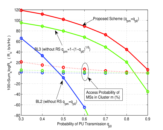
Figure 4: $\sum_{k}\log{R_{k}}$ and access probability of MSs in Cluster m ($m=1,\cdots,M$) versus probability of PU transmission $q_{p0}$. $q_{f}=0.2$, $q_{d}=0.8$, $M$=6, $N$=4, $K_{0}$=10, $K_{m}$=5, $I$=0 dB, receive $SNR=10$ dB, $\sigma_{e}^{2}=0.01$.

System Performance versus PU Activities: Figure 4 illustrates the PFS objective $\sum_{k}\log{R_{k}}$ (average sum-log-rate successfully received by each MS) and access probability of MSs in Cluster $m$ ($m=1,\cdots,M$) versus PU activity $q_{p}$ at receive $SNR=10$ dB and $\sigma_{e}^{2}=0.01$. $\sum_{k}\log{R_{k}}$ and access probability decrease with the increase of PU activities. It can be observed that our proposed scheme provides much greater access probability as well as fairness/throughput performance for the MSs at the cell edge compared with baseline 2 and 3 over a wide range of PU activities. This performance gain is contributed by the conventional RS path-loss gain as well as the increase in the access opportunity for MS at the edge.

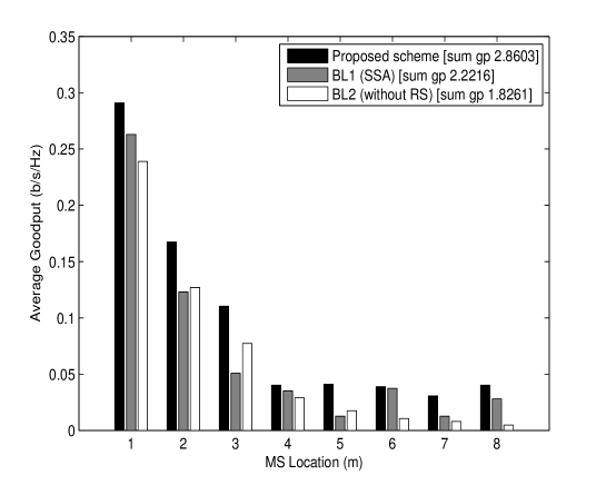
Figure 5: Histogram of the average goodput of MSs (average data rate successfully received at the MSs) at various distance from the BS. $q_{p0}=p_{pm}=0.3$, $q_{f}=0.2$, $q_{d}=0.8$, $M$=6, $N$=4, $K_{0}$=10, $K_{m}$=5, $I$=0 dB, receive $SNR=10$ dB, $\sigma_{e}^{2}=0.01$.

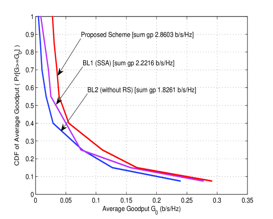
Figure 6: CDF of the average goodput of MSs (average data rate successfully received at the MSs) at various distance from the BS. $q_{p0}=p_{pm}=0.3$, $q_{f}=0.2$, $q_{d}=0.8$, $M$=6, $N$=4, $K_{0}$=10, $K_{m}$=5, $I$=0 dB, receive $SNR=10$ dB, $\sigma_{e}^{2}=0.01$.

Figure 5 illustrates histogram of the average goodput of MSs (average data rate successfully received by the MSs) at various distance from the BS at receive $SNR=10$ dB and $\sigma_{e}^{2}=0.01$. It can be observed that baseline 2 can deliver large system goodput only for those MSs close to the BS. It has very low access probability and average goodput for those far-away mobiles, causing severe fairness issues. However, there is a significant gains in the system goodput of far-away MSs in the proposed system and baseline 1, illustrating both the throughput and fairness advantage of the system with RSs. Furthermore, the proposed scheme outperforms SSA scheme in baseline 1. Figure 6 illustrates the corresponding CDF of average goodput of MSs at various distance. The low average goodput regime ($x$-axis) demonstrates the performance of cell-edge users: the larger probability ($y$-axis) in low average goodput regime the larger average goodput of the cell-edge users. It can be observed that our proposed scheme brings better performance (larger average goodput to the cell-edge users and sum average goodput of all users ) compared with the baselines.

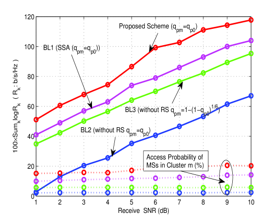
Figure 7: $\sum_{k}\log{R_{k}}$ and access probability of MSs in Cluster m ($m=1,\cdots,M$) versus receive $SNR$. $q_{p0}=0.3$,$q_{f}=0.2$, $q_{d}=0.8$, $M$=6, $N$=4, $K_{0}$=10, $K_{m}$=5, $I$=0 dB, $\sigma_{e}^{2}=0.01$.

System Performance versus Receive SNR: Figure 7 illustrates the PFS objective $\sum_{k}\log{R_{k}}$ (average sum-log-rate successfully received by each MS) and access probability of MSs in Cluster m ($m=1,\cdots,M$) versus receive $SNR$. It can be observed that our proposed design has significant gain over the baseline 1, 2 and 3 systems. The gain is more prominent at low SNR region because the conventional RS reduce the path loss greatly and utilizes the limited power more efficiently.

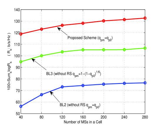
Figure 8: $\sum_{k}\log{R_{k}}$ versus the number of MSs in a cell. $q_{p0}=0.3$, $q_{f}=0.2$, $q_{d}=0.8$, $M$=6, $N$=4, $I$=0 dB, receive $SNR=10$ dB, $\sigma_{e}^{2}=0.01$.

System Performance versus the Number of MSs: Figure 8 illustrates $\sum_{k}\log{R_{k}}$ (average sum-log-rate successfully received by each MS) versus the number of MSs in a cell at receive $SNR=10$ dB and $\sigma_{e}^{2}=0.01$. The ratio between $K_{0}$ and $K_{m}$ is kept constant. While the proposed scheme has the best performance over baseline 2 and 3, the performance of all the three schemes increases with K, which demonstrated the multi-user diversity gain in the system.

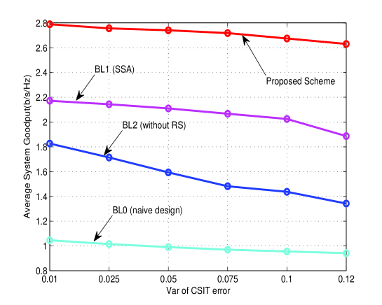
Figure 9: Average system goodput (average data rate successfully received at the MSs) versus CSIT quality. $q_{p0}=p_{pm}=0.3$, $q_{f}=0.2$, $q_{d}=0.8$, $M$=6, $N$=4, $K_{0}$=10, $K_{m}$=5, $I$=0 dB, receive $SNR=10$ dB.

System Performance versus CSIT quality: Figure 9 illustrates the average system goodput (average data rate successfully received by the MS) versus CSIT quality. The performance gain of the proposed scheme versus baseline 1 illustrates the robustness of the proposed scheme w.r.t. CSIT errors. On the other hand, comparison between baseline 2 and baseline 0 illustrated that it is very important to take CSIT errors into the design. Baseline 0 has very poor performance because there are a lot of error packets due to channel outage.

VII Conclusion

In this paper, we have proposed the design of downlink two-hop relay-assisted cognitive OFDMA system, which has the cluster-based architecture and dynamically shares the spectrum of PU systems. Optimal decentralized algorithms have been derived for joint rate and power control, and subchannel allocation at the RS and the BS respectively. These algorithms maximize the weighted system goodput where proportional fair is included as a special case. The solution processed local system state measurement at the BS and the RS to compute (locally) the power, rate and subchannel allocations of the BS and RS. Imperfect system state measurement has been taking into consideration to maintain robust performance of the SU and the PU systems. Significant throughput gains have been observed from simulation results. We have also derived a simple (asymptotically optimal) control algorithm as well as the closed-form performance for PFS for sufficiently large number of users.

Appendix A: Solution of Subproblem 1 and Subproblem 2

The gradient of $L_{m}$ in subproblem 1 vanishes at the maximum, so we have

$$\frac{\partial{L_{m}}}{\partial{p_{m,n,k}}}=0\Rightarrow p_{m,n,k} = \alpha_{m,n,k}\bigg{(}\frac{\frac{1}{4}\big{(}(1-\epsilon)\beta_{m,n}w_{m,k}-\mu_{k}\big{)}}{ln2\big{(}\nu+\eta_{n}\tau^{2}_{m,n}(1-\beta_{m,n})\big{)}}-\frac{1}{\varphi_{m,n,k}}\bigg{)}^{+}$$

$$\frac{\partial{L_{m}}}{\partial{\alpha_{m,n,k}}}=0\Rightarrow X_{m,n,k} \triangleq \frac{1}{4}\big{(}(1-\epsilon)\beta_{m,n}w_{m,k}-\mu_{k}\big{)}\bigg{(}log_{2}(1+\frac{p_{m,n,k}\varphi_{m,n,k}}{\alpha_{m,n,k}})$$ (17)

$$-\frac{p_{m,n,k}\varphi_{m,n,k}}{ln2\left(\alpha_{m,n,k}+p_{m,n,k}\varphi_{m,n,k}\right)}\bigg{)}=\lambda_{n}$$

and $X_{m,n,k}$ can be interpreted as marginal benefit of extra bandwidth. For a particular $\nu$, if there is a unique $k^{*}=\arg\max\{X_{m,n,k}\}$ for some $n$, time-sharing will not happen in this subchannel.

$$\alpha_{m,n,k} = \left\{\begin{array}[]{ll}1,&X_{m,n,k}=\max_{k}\big{\{}X_{m,n,k}\big{\}}>0\\ 0,&\textrm{otherwise}\end{array}\right.$$ (20)

Since for each given $\mu$, $X_{m,n,k}$ is a function of the CSI $\varphi_{m,n,k}$, they are independent random variable. As a result, there is probability 1 that one subchannel is assigned to a single user.

We use the subgradient method to update the multipliers as follows

$$\lambda_{n}(i+1) = \bigg{[}\lambda_{n}(i)-\delta(i)\big{(}1-\sum_{k=1}^{K_{m}}\alpha_{m,n,k}\big{)}\bigg{]}_{\chi}\forall n$$

$$\nu(i+1) = \bigg{[}\nu(i)-\delta(i)\big{(}P_{m}-\sum_{n=1}^{N}\sum_{k=1}^{K_{m}}p_{m,n,k}\big{)}\bigg{]}_{\chi}$$

$$\eta_{n}(i+1) = \bigg{[}\eta_{n}(i)-\delta(i)\big{(}I_{m,n}-\sum_{k=1}^{K_{m}}(1-\beta_{m,n})\tau^{2}_{m,n}p_{m,n,k}\big{)}\bigg{]}_{\chi}\forall n$$

$$\mu_{k}(i+1) = \bigg{[}\mu_{k}(i)-\delta(i)\big{(}R_{m,k}-\sum_{n=1}^{N}\frac{\alpha_{m,n,k}}{4}log(1+\frac{p_{m,n,k}\varphi_{m,n,k}}{\alpha_{m,n,k}})\big{)}\bigg{]}_{\chi}\forall k$$

where $\{\delta(i)\}$ is a sequence of scalar step size and $\chi$ denotes the projection onto the feasible set, which contains all non-negative real numbers. The iterative algorithm terminates when the difference of two consecutive multipliers is less than a terminating threshold. The subgradient update is guaranteed to converge to the optimal multipliers $\lambda_{n}^{*},\nu^{*},\eta_{n}^{*},\mu_{k}^{*}$.

We form the Lagrangian of Subproblem 2 as follows

$$L_{0} = \widetilde{G}_{0}+\sum_{m=1}^{M}\sum_{n=1}^{N}(1-\epsilon)\beta_{0,n}\widetilde{G}_{n,m}^{*}-\sum_{n=1}^{N}\lambda_{n}\left(\sum_{k=1}^{K_{0}}\alpha_{0,n,k}-1\right)$$ (21)

$$-\nu\left(\sum_{n=1}^{N}\sum_{k=1}^{K_{0}}p_{0,n,k}-P_{0}\right)-\sum_{n=1}^{N}\eta_{n}\left(\sum_{k=1}^{K_{0}}(1-\beta_{0,n})\tau^{2}_{0,n}p_{0,n,k}-I_{0,n}\right)$$

$$\frac{\partial{L_{0}}}{\partial{p_{0,n,k}}}=0 \Rightarrow p_{0,n,k}=\alpha_{0,n,k}(\frac{\frac{1}{2}(1-\epsilon)\beta_{0,n}w_{0,k}}{ln2\big{(}\nu+\eta_{n}\tau^{2}_{0,n}(1-\beta_{0,n})\big{)}}-\frac{1}{\varphi_{0,n,k}})^{+}$$

$$\frac{\partial{L_{0}}}{\partial{\alpha_{0,n,k}}}=0 \Rightarrow X_{0,n,k}\triangleq\frac{1}{2}(1-\epsilon)\beta_{0,n}w_{0,k}\bigg{(}log_{2}(1+\frac{p_{0,n,k}\varphi_{0,n,k}}{\alpha_{0,n,k}})-\frac{p_{0,n,k}\varphi_{0,n,k}}{ln2\big{(}\alpha_{0,n,k}+p_{0,n,k}\varphi_{0,n,k}\big{)}}\bigg{)}=\lambda_{n}$$

$$\alpha_{0,n,k} = \left\{\begin{array}[]{ll}1,&X_{0,n,k}=\max_{k}\big{\{}X_{0,n,k}\big{\}}>0\\ 0,&\textrm{otherwise}\end{array}\right.$$ (24)

where $w_{0,k}(k=1,\cdots,M)$ is the derivative on $\widetilde{G}_{m}^{*}$ w.r.t. $r_{0,n,m}$ which can be interpreted as the equivalent weight of the $m$-th RS. As a result, we can use similar subgradient update procedure as in (Appendix A: Solution of Subproblem 1 and Subproblem) to obtain the multipliers $\lambda_{n}(i),\nu(i),\eta_{n}(i)$. Furthermore, when the data rates for the relay stations are determined, the packet partition factors $\{d_{m,n,k}\}$ can be determined according to the structure of $\tilde{G}_{m}^{**}(\cdot)$. Thus, select the best packet partition factors which can achieve the curve of $\tilde{G}_{m}^{**}(\cdot)$.

Appendix B: Proof of Lemma 1

According to Appendix A, it with probability $1$ that one subchannel is allocated to only one user or relay station in phase one. Moreover, since channel between the base station and relay station is good enough, one subchannel is sufficient to carry the data for the phase two transmission. Therefore, it with probability $1$ that one relay is allocated at most one subchannel. Thus, for any relay station, there is only one positive value in the set of rate allocation $\{r_{0,n,m}|\forall n\}$. Notice that $\tilde{G}_{m}^{**}(0)=0,$ we have

$$\tilde{G}_{m}^{**}(\sum_{n}r_{0,n,m}t_{n,m}|\hat{\mathbf{S}}_{m},\hat{\mathbf{H}}_{m}) = \sum_{n=1}^{N}\tilde{G}_{m}^{**}(r_{0,n,m}t_{n,m}|\hat{\mathbf{S}}_{m},\hat{\mathbf{H}}_{m})$$

$$= \sum_{n=1}^{N}t_{n,m}\tilde{G}_{m}^{**}(r_{0,n,m}|\hat{\mathbf{S}}_{m},\hat{\mathbf{H}}_{m})\quad\forall m.$$

Hence,

$$\mathbf{E}_{\mathbf{T}_{m}}\tilde{G}_{m}^{**}(\sum_{n}r_{0,n,m}t_{n,m}|\hat{\mathbf{S}}_{m},\hat{\mathbf{H}}_{m}) = \sum_{n=1}^{N}\mathbf{E}_{t_{n,m}}t_{n,m}\tilde{G}_{m}^{**}(r_{0,n,m}|\hat{\mathbf{S}}_{m},\hat{\mathbf{H}}_{m})$$ (25)

$$= \sum_{n=1}^{N}(1-\epsilon)\beta_{0,n}\tilde{G}_{m}^{**}(r_{0,n,m}|\hat{\mathbf{S}}_{m},\hat{\mathbf{H}}_{m})$$

This complete the proof.

Appendix C: Proof of Lemma 2

Without loss of generality, we consider the $m$-th cluster. Suppose there are $L$ QoS classes and denote $w_{l}$ as the weight of the $l$-th QoS class. Since there is sufficiently large number of users in each cluster, the receiving SNR of the selected users will be sufficiently large, therefore, equal power allocation is asymptotically optimal. Moreover, since the relay station is only likely to pick up the best users (with the largest) from each QoS class, and the channel fading of the best user tends to be a constant (e.g. $\ln K$) when the number of users is sufficiently large, which subchannel is allocated to which QoS class become independent of the channel fading. Hence, the optimal resource allocation is to do time-sharing among the $L$ class.

Let $g_{m,l}$ denote the maximum average weighted throughput of the $m$-th cluster if there are sufficient information bits at the relay and only the users of the $l$-th QoS class are scheduled, and $\{r_{m,n,k}^{l}\}$ be the rate allocation leading to the maximum average weighted throughput $g_{m,l}$. We define $r_{m,l}=\sum_{n,k}r_{m,n,k}^{l}$ denoting the corresponding total transmit data rate. These two parameters can be evaluated by each relay locally. We first construct a function of $\mathcal{G}_{m}(r)$ ($\mathcal{G}_{m}:\mathcal{R}\rightarrow\mathcal{R}$) below (An example of $\mathcal{G}_{m}(r)$ is shown in Figure 3):

• Plot points $\{(r_{m,l},g_{m,l})|\forall l\}$ on a plane. This refers to the points B and C in Figure 3.

• Let $\mathcal{H}$ be the convex hull of the points $\{(r_{m,l},g_{m,l})|\forall l\}$ and $(0,0)$. This refers to the triangle ABC in Figure 3.

• Define a region $\widetilde{\mathcal{H}}$ as $\widetilde{\mathcal{H}}=\{(r,g)|\exists(r,g_{e})\in\mathcal{H},\ g_{e}\leq g\}$. This refers to the area bounded by line ABCD and x-axis in Figure 3. Therefore, for any given $r$, all the average weighted throughput in the set $\{g|(r,g)\in\widetilde{\mathcal{H}}\}$ can is achievable by the cluster $m$ using TDMA in each frame.

• $\mathcal{G}_{m}(r)=\max\{g|(r,g)\in\widetilde{\mathcal{H}}\}$. This refers to the line ABCD in Figure 3.

An example of Therefore, $\widetilde{G}_{m}^{**}(r)\geq\mathcal{G}_{m}(r)$. Moreover, since $\frac{\widetilde{G}_{m}^{**}(r)-\mathcal{G}_{m}(r)}{\mathcal{G}_{m}(r)}\rightarrow 0$ for sufficiently large number of users in each QoS class, it’s asymptotically optimal to have $\widetilde{G}_{m}^{**}(r)=\mathcal{G}_{m}(r)$.

Appendix D: Proof of Lemma 3

Without loss of generality, we consider the $m$-th cluster. Since the number of MSs in the $m$-th cluster $K_{m}$ is sufficiently large, the sensing measure $\beta_{m,n}\rightarrow S_{m,n}$ and the system is working on the high SNR regime. Therefore, the throughput gain of power allocation across the subchannels is negligible and we can simply assign equal power to each available subchannel, thus $p_{m,n}=\frac{\beta_{m,n}}{\sum_{n=1}^{N}\beta_{m,n}}P_{0}$.

We first consider the case where $r\geq R_{m}=\sum_{m=1}^{M}\log_{2}\left(1+p_{m,n}l_{m,n,k}\varphi_{m,n,k}\right)$. In this case, there are sufficient information bits at the relay for phase two transmission. Then the selected MS of the $n$-th subchannel and the $m$-th cluster is given by $A_{m,n}=\arg\max_{k}w_{m,k}\log_{2}\left(1+p_{m,n}l_{m,n,k}\varphi_{m,n,k}\right)$, and $\widetilde{G}_{m}^{**}(r)=\sum_{n=1}^{N}\frac{w_{m,A_{m,n}}\beta_{m,n}(1-\epsilon)}{4}\log_{2}(1+p_{m,n}l_{m,n,A_{m,n}}\varphi_{m,n,A_{m,n}})$.

For the case where $r<R_{m}$, it’s easy to see by linear interpolation that $\widetilde{G}_{m}^{**}(r)\geq\\ \sum_{n=1}^{N}\frac{rw_{m,A_{m,n}}\beta_{m,n}(1-\epsilon)}{4R_{m}}\log_{2}(1+p_{m,n}l_{m,n,A_{m,n}}\varphi_{m,n,A_{m,n}})$. However, since the BS-RS link is sufficiently good, the BS always delivers $R_{m}$ bits to the $m$-th relay. Hence, we can simply let $\widetilde{G}_{m}^{**}(r)=\\ \sum_{n=1}^{N}\frac{rw_{m,A_{m,n}}\beta_{m,n}(1-\epsilon)}{4R_{m}}\log_{2}(1+p_{m,n}l_{m,n,A_{m,n}}\varphi_{m,n,A_{m,n}})$, which does not affect the scheduling results at the BS.

Appendix E: Proof of Theorem 1

Due to page limitation, we provide a sketch of proof. When the RS-BS link is sufficiently good due to the existence of line-of-sight path, the relay will always receive sufficiently information bits as long as there is one available subchannel in cluster $0$, and the PFS algorithm in each relay cluster works as that in single cell systems with infinite backlog. Hence, we can follow the similar approach as in [27] to prove that when $K_{c}$ is sufficiently large, the user selection is based on the small-scale channel fading, which leads to (15).

Since there are $N$ subchannels in the system, the probability the BS can not deliver packets to the relays is $q_{p}^{N}$. Hence, in each cluster the probability one subchannel is used to deliver packet is $(1-q_{p})(1-q_{p}^{N})$. Again, by following the similar approach as in [27], the $\overline{T}_{m,k}$ can be derived after some algebra.

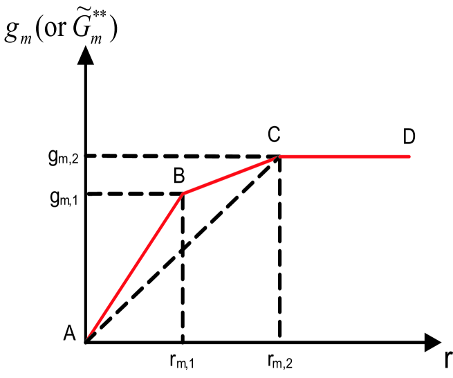
Figure 3: An example of function $\widetilde{G}_{m}^{**}$ where there are two QoS classes with weights $w_{1}$, $w_{2}$ and maximum achievable data rate $r_{m,1}$ ,$r_{m,2}$. The x-axis is the number of information bits the RS decoded in phase one, and the y-axis is the maximum average weighted goodput achieved by this RS. When the number of information bits is less than $r_{m,1}$, only the first QoS class is scheduled; when it’s larger than $r_{m,1}$ but less than $r_{m,2}$, both two classes are scheduled by TDMA; and when it’s larger than $r_{m,2}$, only the second QoS class is scheduled.

References

- [1] I. F. Akyildiz, W. Lee, M. C. Vuran, and S. Mohanty, “Next generation/dynamic spectrum access/cognitive radio wireless networks: a survey,” Computer Networks, vol. 50, no. 13, pp. 2127–2159, 2006.
- [2] J. Huang, R. Berry, and M. L. Honig, “Auction-based spectrum sharing,” ACM Mobile Networks and Applications Journal (MONET), vol. 11, pp. 405–418, June 2006.
- [3] S. Sharma and D. Teneketzis, “An externality-based decentralized optimal power allocation scheme for wireless mesh networks,” 4th Annual IEEE Communications Society Conference on Sensor, Mesh and Ad Hoc Communications and Networks, 2007 (SECON ’07), pp. 284–293, 18-21 June 2007.
- [4] Q. Zhao, S. Geirhofer, L. Tong, and B. Sadler, “Opportunistic spectrum access via periodic channel sensing,” IEEE Transactions on Signal Processing, vol. 56, no. 2, pp. 785–796, Feb. 2008.
- [5] H. Islam, Y. chang Liang, and A. Hoang, “Joint power control and beamforming for cognitive radio networks,” IEEE Transactions on Wireless Communications, vol. 7, pp. 2415–2419, July 2008.
- [6] W. Nam, W. Chang, S.-Y. Chung, and Y. Lee, “Transmit optimization for relay-based cellular ofdma systems,” IEEE International Conference on Communications, 2007 (ICC ’07), pp. 5714–5719, June 2007.
- [7] O. Oyman, “Opportunistic scheduling and spectrum reuse in relay-based cellular ofdma networks,” IEEE Global Telecommunications Conference, 2007 (GLOBECOM ’07), pp. 3699–3703, Nov. 2007.
- [8] G. Li and H. Liu, “Resource allocation for ofdma relay networks with fairness constraints,” IEEE Journal on Selected Areas in Communications, vol. 24, pp. 2061–2069, Nov. 2006.
- [9] T. C.-Y. Ng and W. Yu, “Joint optimization of relay strategies and resource allocations in cooperative cellular networks,” IEEE Journal on Selected Areas in Communications, vol. 25, no. 2, pp. 328–339, February 2007.
- [10] M. Awad and X. Shen, “Ofdma based two-hop cooperative relay network resources allocation,” IEEE International Conference on Communications, 2008 (ICC ’08), pp. 4414 –4418, may 2008.
- [11] B. Can, H. Yanikomeroglu, F. Onat, E. De Carvalho, and H. Yomo, “Efficient cooperative diversity schemes and radio resource allocation for ieee 802.16j,” IEEE Wireless Communications and Networking Conference, 2008 (WCNC ’08), pp. 36 –41, 31 2008-april 3 2008.
- [12] Z. Tang and G. Wei, “Resource allocation with fairness consideration in ofdma-based relay networks,” IEEE Wireless Communications and Networking Conference, 2009 (WCNC ’09), pp. 1 –5, april 2009.
- [13] G. Calcev and J. Bonta, “Ofdma cellular networks with opportunistic two-hop relays,” EURASIP Journal on Wireless Communications and Networking, vol. 2009, 2009.
- [14] H. Li, H. Luo, X. Wang, C. Lin, and C. Li, “Fairness-aware resource allocation in ofdma cooperative relaying network,” IEEE International Conference on Communications, 2009 (ICC ’09), pp. 1 –5, june 2009.
- [15] K. Park, H. S. Ryu, C. G. Kang, D. Chang, S. Song, J. Ahn, and J. Ihm, “The performance of relay-enhanced cellular ofdma-tdd network for mobile broadband wireless services,” EURASIP J. Wirel. Commun. Netw., vol. 2009, pp. 1–10, 2009.
- [16] M. K. Kim and H. S. Lee, “Radio resource management for a two-hop OFDMA relay system in downlink,” IEEE Symposium on Computers and Communications, pp. 25 – 31, 2007.
- [17] A. Goldsmith, Wireless Communications. Cambridge University Press, 2005.
- [18] T. L. Marzetta and B. M. Hochwald, “Fast transfer of channel state information in wireless systems,” IEEE Transactions on Signal Processing, vol. 54, pp. 1268–78, Apr. 2006.
- [19] S. Lim, S. Kim, C. Park, and M. Song, “The detection and classification of the wireless microphone signal in the ieee 802.22 wran system,” Asia-Pacific Microwave Conference, 2007. APMC 2007., pp. 1 –4, dec. 2007.
- [20] Q. Zhao and B. M. Sadler, “A survey of dynamic spectrum access,” IEEE Signal Processing Magazine, vol. 24, pp. 79–89, May 2007.
- [21] S. Y. Chung, R. Urbanke, and T. J. Richardson, “Gaussian approximation for sum-product decoding of low-density parity-check codes,” Proceedings of International Symposium in Information Theory, pp. 318–319, Jun. 2000.
- [22] D. Palomar and M. Chiang, “Alternative distributed algorithms for network utility maximization: Framework and applications,” Automatic Control, IEEE Transactions on, vol. 52, no. 12, pp. 2254–2269, Dec. 2007.
- [23] S. Boyd and L. Vandenberghe, Convex Optimization. Cambridge, UK: Cambridge, 2004.
- [24] W. Yu and R. Lui, “Dual methods for nonconvex spectrum optimization of multicarrier systems,” IEEE Transactions on Communications, vol. 54, no. 7, pp. 1310–1322, July 2006.
- [25] “Requirement for evolved UTRA (E-UTRA) and evolved UTRAN (E-URTAN),” 3GPP TR 25.913, Dec. 2009.
- [26] “IEEE 802.16m evaluation methodology document.” IEEE 802.16m-08/004r5.
- [27] G. Caire, R. Muller, and R. Knopp, “Hard fairness versus proportional fairness in wireless communications: The single-cell case,” Information Theory, IEEE Transactions on, vol. 53, pp. 1366–1385, April 2007.