Gaussian Z-Interference Channel with a Relay Link: Achievability Region and Asymptotic Sum Capacity

Abstract

This paper studies a Gaussian Z-interference channel with a rate-limited digital relay link from one receiver to another. Achievable rate regions are derived based on a combination of Han-Kobayashi common-private power splitting technique and either a compress-and-forward relay strategy or a decode-and-forward strategy for interference subtraction at the other end. For the Gaussian Z-interference channel with a digital link from the interference-free receiver to the interfered receiver, the capacity region is established in the strong interference regime; an achievable rate region is established in the weak interference regime. In the weak interference regime, the decode-and-forward strategy is shown to be asymptotically sum-capacity achieving in the high signal-to-noise ratio and high interference-to-noise ratio limit. In this case, each relay bit asymptotically improves the sum capacity by one bit. For the Gaussian Z-interference channel with a digital link from the interfered receiver to the interference-free receiver, the capacity region is established in the strong interference regime; achievable rate regions are established in the moderately strong and weak interference regimes. In addition, the asymptotic sum capacity is established in the limit of large relay link rate. In this case, the sum capacity improvement due to the digital link is bounded by half a bit when the interference link is weaker than a certain threshold, but the sum capacity improvement becomes unbounded when the interference link is strong.

I Introduction

The classic interference channel models a communication situation in which two transmitters communicate with their respective intended receivers while mutually interfering with each other. The interference channel is of fundamental importance for communication system design, because many practical systems are designed to operate in the interference-limited regime. The largest known achievability region for the interference channel is due to Han and Kobayashi [1], where a common-private power splitting technique is used to partially decode and subtract the interfering signal. The Han-Kobayashi scheme has been shown to be capacity achieving in a very weak interference regime [2, 3, 4] and to be within one bit of the capacity region in general [5].

This paper considers a communication model in which the classic interference channel is augmented by a noiseless relay link between the two receivers. We are motivated to study such a relay-interference channel because in practical wireless cellular systems, the uplink receivers at the base-stations are connected via backhaul links and the downlink receivers may also be capable of establishing an independent communication link for the purpose of interference mitigation.

\psfrag{X1}{$X_{1}$}\psfrag{X2}{$X_{2}$}\psfrag{Z1}{$Z_{1}$}\psfrag{Z2}{$Z_{2}$}\psfrag{Y1}{$Y_{1}$}\psfrag{Y2}{$Y_{2}$}\psfrag{h11}{$h_{11}$}\psfrag{h22}{$h_{22}$}\psfrag{h21}{$h_{21}$}\psfrag{h12}{$h_{12}$}\psfrag{R21}{$R_{21}$}\psfrag{R12}{$R_{12}$}\psfrag{R0}{$R_{0}$}\psfrag{(a) Type I}{(a) Type I}\psfrag{(b) Type II}{(b) Type II}\includegraphics[width=140.92627pt]{./figures/relay_ic_type_i}

\psfrag{X1}{$X_{1}$}\psfrag{X2}{$X_{2}$}\psfrag{Z1}{$Z_{1}$}\psfrag{Z2}{$Z_{2}$}\psfrag{Y1}{$Y_{1}$}\psfrag{Y2}{$Y_{2}$}\psfrag{h11}{$h_{11}$}\psfrag{h22}{$h_{22}$}\psfrag{h21}{$h_{21}$}\psfrag{h12}{$h_{12}$}\psfrag{R21}{$R_{21}$}\psfrag{R12}{$R_{12}$}\psfrag{R0}{$R_{0}$}\psfrag{(a) Type I}{(a) Type I}\psfrag{(b) Type II}{(b) Type II}\includegraphics[width=140.92627pt]{./figures/relay_ic_type_ii}

Figure 1: Gaussian Z-interference channel with a relay link: (a) Type I; (b) Type II.

This paper explores the use of relay techniques for interference mitigation. We focus on the simplest interference channel model, the Gaussian Z-interference channel (also known as the one-sided interference channel), in which one of the receivers gets an interference-free signal, the other receiver gets a combination of the intended and the interfering signals, and the channel is equipped with a noiseless link of fixed capacity from one receiver to the other. The Z-interference channel is of practical interest because it models a two-cell cellular network with one user located at the cell edge and another user at the cell center. (The cell-edge user is sometimes referred to as in a soft-handoff mode [6].) Depending on the direction of the noiseless link, the proposed model is named the Type I or the Type II Gaussian Z-relay-interference channel in this paper as shown in Fig. 1.

The Type I Gaussian Z-relay-interference channel has a digital relay link of finite capacity from the interference-free receiver to the interfered receiver. Our main coding strategy for the Type I channel is a decode-and-forward strategy, in which the relay link forwards part of the interference to the interfered receiver using a binning technique for interference subtraction. This paper shows that decode-and-forward is capacity achieving for the Type I channel in the strong interference regime, and is asymptotically sum-capacity achieving in the weak interference regime. In addition, in the weak interference regime, every bit of relay link rate increases the sum rate by one bit in the high signal-to-noise ratio (SNR) and high interference-to-noise ratio (INR) limit.

The Type II Gaussian Z-relay-interference channel differs from the Type I channel in that the direction of the digital link goes from the interfered receiver to the interference-free receiver. Our main coding strategy for the Type II channel is based on a combination of two relaying strategies: decode-and-forward and compress-and-forward. In the proposed scheme, the interfered receiver, which decodes the common message and observes a noisy version of the neighbor’s private message, describes the common message with a bin index and describes the neighbor’s private message using a quantization scheme. It is shown that, in the strong interference regime, a special form of the proposed relaying scheme, which uses decode-and-forward only, is capacity achieving. In the weak interference regime, the proposed scheme reduces to pure compress-and-forward. Further, when the interference link is weaker than a certain threshold, the sum-capacity gain due to the digital link for the Type II channel is upper bounded by half a bit. This is in contrast to the Type I channel, in which each relay bit can be worth up to one bit in sum capacity.

I-A Related Work

The Gaussian Z-interference channel has been extensively studied in the literature. It is one of the few examples of an interference channel (besides the strong interference case [1, 7, 8] and the very weak interference case [2, 3, 4]) for which the sum capacity has been established. The sum capacity of the Gaussian Z-interference channel in the weak interference regime is achieved with both transmitters using Gaussian codebooks and with the interfered receiver treating the interference as noise [5, 9].

The fundamental decode-and-forward and compress-and-forward strategies for the relay channel are due to the classic work of Cover and El Gamal [10]. Our study of the interference channel with a relay link is motivated by the more recent capacity results for a class of deterministic relay channels investigated by Kim [11] and a class of modulo-sum relay channels investigated by Aleksic et al. [12], where the relay observes the noise in the direct channel. The situation investigated in [11, 12] is similar to the Type I Gaussian Z-relay-interference channel, where the interference-free receiver observes a noisy version of the interference at the interfered receiver and helps the interfered receiver by describing the interference through a noiseless relay link.

The channel model studied in the paper is related to the work of Sahin et al. [13, 14, 15], Marić et al. [16], Dabora et al. [17], and Tian and Yener [18], where the achievable rate regions and the relay strategies are studied for an interference channel with an additional relay node, and where the relay observes the transmitted signals from the inputs and contributes to the outputs of both channels. In particular, [16], [17] propose an interference-forwarding strategy which is similar to the one used for the Type I channel in this paper. In a similar setup, the works of Ng et al. [19] and Høst-Madsen [20] study the interference channel with analog relay links at the receiver, and use the compress-and-forward relay strategy to obtain capacity bounds and asymptotic results.

This paper is closely related to the work of Wang and Tse [21], Prabhakaran and Viswanath [22], and Simeone et al. [23], where the interference channel with limited receiver cooperation is studied. In [23], the achievable rates of a Wyner-type cellular model with either uni- or bidirectional finite-capacity backhaul links are characterized. In [21], a more general channel model in which a two-user Gaussian interference channel is augmented with bidirectional digital relay links is considered, and a conferencing protocol based on the quantize-map-and-forward strategy of [24] is proposed.

The present paper considers a special case of the channel model in [21], i.e., a simplified Gaussian Z-interference channel model with a unidirectional digital relay link. By focusing on this special case, we are able to derive concrete achievability results and upper bounds and obtain insights on the rate improvement due to the relay link. For example, while [21] adopts a universal power splitting ratio of [5] at the transmitter to achieve the capacity region to within 2 bits, this paper adapts the power splitting ratio to channel parameters, and shows that in the weak interference regime a relay link from the interference-free receiver to the interfered receiver is much more beneficial than a relay link in the opposite direction for a Z-interference channel.

I-B Outline of the Paper

The rest of this paper is organized as follows. Section II presents achievability results for the Type I Gaussian Z-relay-interference channel using the decode-and-forward strategy. Capacity results are established for the strong interference regime; asymptotic sum-capacity result is established for the weak interference regime in the high SNR/INR limit. Section III presents achievability results for the Type II Gaussian Z-relay-interference channel using a combination of the decode-and-forward scheme and the compress-and-forward scheme. Capacity results are derived in the strong interference regimes; asymptotic sum-capacity result is established for all channel parameters in the limit of large relay link rate. Section IV contains concluding remarks.

II Gaussian Z-Interference Channel with
a Relay Link: Type I

II-A Channel Model and Notations

The Gaussian Z-interference channel is modeled as follows (see Fig. 1(a)):

$$\left\{\begin{array}[]{l}Y_{1}=h_{11}X_{1}+h_{21}X_{2}+Z_{1}\\ Y_{2}=h_{22}X_{2}+Z_{2}\end{array}\right.$$ (1)

where $X_{1}$ and $X_{2}$ are the transmit signals with power constraints $P_{1}$ and $P_{2}$ respectively, $h_{ij}$ represents the real-valued channel gain from transmitter $i$ to receiver $j$, and $Z_{1}$, $Z_{2}$ are the independent additive white Gaussian noises (AWGN) with power $N$. In addition, the Type I Gaussian Z-relay-interference channel is equipped with a digital noiseless link of fixed capacity $R_{0}$ from receiver 2 to receiver $1$.

Each transmitter $i$ independently encodes a message $m_{i}$ into a codeword $X_{i}^{n}(m_{i})$ using a codebook $\mathcal{C}_{i}^{n}$ of $2^{nR_{i}}$ length-$n$ codewords satisfying an average power constraint $P_{i}$. Let $V^{n}$ be the output of the digital link from receiver $2$ to receiver $1$ taken from a relay codebook $\mathcal{C}_{R}^{n}$, where $|\mathcal{C}_{R}^{n}|\leq 2^{nR_{0}}$. Receiver $1$ uses a decoding function $\hat{m}_{1}=f_{1}^{n}(Y_{1}^{n},V^{n})$. Receiver $2$ uses a decoding function $\hat{m}_{2}=f_{2}^{n}(Y_{2}^{n})$. The average probability of error for user $i$ is defined as $P_{e,i}^{n}=\mathbb{E}\left[\textrm{Pr}(\hat{m}_{i}\neq m_{i})\right]$. A rate pair $(R_{1},R_{2})$ is said to be achievable if for every $\epsilon>0$ and for all sufficiently large $n$, there exists a family of codebooks $(\mathcal{C}_{i}^{n},\mathcal{C}_{R}^{n})$, and decoding functions $f_{i}^{n}$, $i=1,2$, such that $\max_{i}\{P_{e,i}^{n}\}<\epsilon$. The capacity region is defined as the set of all achievable rate pairs.

To simplify the notation, the following definitions are used throughout this paper:

$$\mathsf{SNR_{1}}=\frac{|h_{11}|^{2}P_{1}}{N} \mathsf{SNR_{2}}=\frac{|h_{22}|^{2}P_{2}}{N}$$

$$\mathsf{INR_{2}}=\frac{|h_{21}|^{2}P_{2}}{N} \gamma(x)=\frac{1}{2}\log(1+x)$$

where $\log(\cdot)$ is base 2. In addition, denote $\overline{\beta}=1-\beta$, and let $(x)^{+}=\max\{x,0\}$.

II-B Achievable Rate Region

This paper uses a combination of the Han-Kobayashi common-private power splitting technique and a decode-and-forward strategy for the Gaussian Z-relay-interference channel, in which a common information stream is decoded at receiver $2$, then binned and forwarded to receiver $1$ for subtraction. The main result of this section is the following achievability theorem.

Theorem 1

For the Type I Gaussian Z-interference channel with a digital relay link of limited rate $R_{0}$ from the interference-free receiver to the interfered receiver as shown in Fig. 1(a), in the weak interference regime defined by $0\leq\mathsf{INR_{2}}<\min\{\mathsf{SNR_{2},INR_{2}^{*}}\}$, the following rate region is achievable:

$$\bigcup_{0\leq\beta\leq 1}\left\{(R_{1},R_{2})\left|R_{1}\leq\gamma\left(\frac{\mathsf{SNR}_{1}}{1+\beta\mathsf{INR}_{2}}\right),\right.\right.\\ R_{2}\leq\min\left\{\gamma(\mathsf{SNR}_{2}),\gamma(\beta\mathsf{SNR}_{2})+\right.\\ \left.\left.\gamma\left(\frac{\overline{\beta}\mathsf{INR}_{2}}{1+\mathsf{SNR}_{1}+\beta\mathsf{INR}_{2}}\right)+R_{0}\right\}\right\},$$ (2)

where

$$\mathsf{INR_{2}^{*}}=\left((1+\mathsf{SNR}_{1})(2^{-2R_{0}}\mathsf{(1+SNR_{2})}-1)\right)^{+}.$$ (3)

In the strong interference regime defined by $\min\{\mathsf{SNR_{2},INR_{2}^{*}}\}\leq\mathsf{INR_{2}}<\mathsf{INR}_{2}^{*}$, the capacity region is given by

$$\left\{(R_{1},R_{2})\left|\begin{array}[]{rll}R_{1}&\leq&\gamma(\mathsf{SNR_{1}})\\ R_{2}&\leq&\gamma(\mathsf{SNR_{2}})\\ R_{1}+R_{2}&\leq&\gamma(\mathsf{SNR_{1}+INR_{2}})+R_{0}\end{array}\right.\right\}.$$ (4)

In the very strong interference regime defined by $\mathsf{INR_{2}\geq INR_{2}^{*}}$, the capacity region is given by

$$\left\{(R_{1},R_{2})\left|\begin{array}[]{l}R_{1}\leq\gamma(\mathsf{SNR_{1}})\\ R_{2}\leq\gamma(\mathsf{SNR_{2}})\\ \end{array}\right.\right\}.$$ (5)

\psfrag{X1}{$X_{1}$}\psfrag{X2}{$X_{2}$}\psfrag{Y1}{$Y_{1}$}\psfrag{Y2}{$Y_{2}$}\psfrag{U2}{$U_{2}$}\psfrag{W2}{$W_{2}$}\psfrag{Z1}{$Z_{1}$}\psfrag{Z2}{$Z_{2}$}\psfrag{R0}{$R_{0}$}\psfrag{S1}{$S_{1}$}\psfrag{T2}{$T_{2}$}\psfrag{S2}{$S_{2}$}\psfrag{P1}{$P_{1}$}\psfrag{b_P2}{$\overline{\beta}P_{2}$}\psfrag{bP2}{$\beta P_{2}$}\psfrag{h11}{$h_{11}$}\psfrag{h22}{$h_{22}$}\psfrag{h21}{$h_{21}$}\includegraphics[width=238.49121pt]{./figures/hk_relay_ic_type_i}

Figure 2: Common-private power splitting for Type I channel.

Proof:

We use the Han-Kobayashi [1] common-private power splitting scheme with Gaussian inputs to prove the achievability of the rate regions (2), (4) and (5). As depicted in Fig. 2, user $1$’s signal $X_{1}$ is intended for decoding at $Y_{1}$ only. User $2$’s signal $X_{2}$ is the superposition of the private message $U_{2}$ and the common message $W_{2}$, i.e., $X_{2}=U_{2}+W_{2}$. The private message can only be decoded by the intended receiver $Y_{2}$, while the common message can be decoded by both receivers. Independent Gaussian codebooks of sizes $2^{nS_{1}}$, $2^{nS_{2}}$ and $2^{nT_{2}}$ are generated according to i.i.d. Gaussian distributions $X_{1}\sim\mathcal{N}(0,P_{1})$, $U_{2}\sim\mathcal{N}(0,\beta P_{2})$, and $W_{2}\sim\mathcal{N}(0,\overline{\beta}P_{2})$, respectively, where $0\leq\beta\leq 1$. The encoded sequences $X_{1}^{n}$ and $X_{2}^{n}=U_{2}^{n}+W_{2}^{n}$ are then transmitted over a block of $n$ time instances.

Decoding takes place in two steps. First, $(W_{2}^{n},U_{2}^{n})$ are decoded at receiver $2$. The set of achievable rates $(T_{2},S_{2})$ is the capacity region of a Gaussian multiple-access channel, denoted here by $\mathcal{C}_{2}$, where

$$\left\{\begin{array}[]{rll}T_{2}&\leq&\gamma(\overline{\beta}\mathsf{SNR_{2}})\\ S_{2}&\leq&\gamma(\beta\mathsf{SNR_{2}})\\ S_{2}+T_{2}&\leq&\gamma(\mathsf{SNR_{2}}).\end{array}\right.$$ (6)

After $(W_{2}^{n},U_{2}^{n})$ are decoded at receiver $2$, $(X_{1}^{n},W_{2}^{n})$ are then decoded at receiver $1$ with $U_{2}^{n}$ treated as noise, but with the help of the relay link. This is a multiple-access channel with a rate-limited relay $Y_{2}^{n}$, who has complete knowledge of $W_{2}^{n}$. This channel is a special case of the multiple-access relay channel studied in [25] and [26]. It is straightforward to show that a decode-and-forward relay strategy is capacity achieving in this special case and its capacity region $\mathcal{C}_{1}$ is the set of $(S_{1},T_{2})$ for which

$$\left\{\begin{array}[]{rll}S_{1}&\leq&\gamma\left(\displaystyle\frac{\mathsf{SNR_{1}}}{1+\beta\mathsf{INR_{2}}}\right)\\ T_{2}&\leq&\gamma\left(\displaystyle\frac{\overline{\beta}\mathsf{INR_{2}}}{1+\beta\mathsf{INR_{2}}}\right)+R_{0}\\ S_{1}+T_{2}&\leq&\gamma\left(\displaystyle\frac{\mathsf{SNR_{1}}+\overline{\beta}\mathsf{INR_{2}}}{1+\beta\mathsf{INR_{2}}}\right)+R_{0}.\end{array}\right.$$ (7)

An achievable rate region of the Gaussian Z-interference channel with a relay link is then the set of all $(R_{1},R_{2})$ such that $R_{1}=S_{1}$ and $R_{2}=S_{2}+T_{2}$ for some $(S_{1},T_{2})\in\mathcal{C}_{1}$ and $(S_{2},T_{2})\in\mathcal{C}_{2}$. Further, since $\mathcal{C}_{1}$ and $\mathcal{C}_{2}$ depend on the common-private power splitting ratio $\beta$, the convex hull of the union of all such $(R_{1},R_{2})$ sets over all choices of $\beta$ is achievable.

A Fourier-Motzkin elimination method (see e.g. [27]) can be used to show that for each fixed $\beta$, the achievable $(R_{1},R_{2})$’s form a pentagon region characterized by

$$\mathcal{R}_{\beta}=\left\{(R_{1},R_{2})\left|\begin{array}[]{l}\displaystyle R_{1}\leq\gamma\left(\mathsf{\frac{SNR_{1}}{1+\beta INR_{2}}}\right)\\ \displaystyle R_{2}\leq\min\{\gamma(\mathsf{SNR_{2}}),\gamma(\mathsf{\beta SNR_{2}})+\\ \displaystyle\qquad\qquad\quad\gamma\left(\mathsf{\frac{\overline{\beta}INR_{2}}{1+\beta INR_{2}}}\right)+R_{0}\}\\ \displaystyle R_{1}+R_{2}\leq\gamma(\mathsf{\beta SNR_{2}})+\\ \qquad\qquad\quad\gamma\displaystyle\left(\mathsf{\frac{SNR_{1}+\overline{\beta}INR_{2}}{1+\beta INR_{2}}}\right)+R_{0}\\ \end{array}\right.\right\}.$$ (8)

The convex hull of the union of these pentagons over $\beta$ gives the complete achievability region. It happens that the union of the pentagons, i.e. $\bigcup_{0\leq\beta\leq 1}\mathcal{R}_{\beta}$, is already convex. Therefore, convex hull is not needed. In the following, we give an explicit expression for $\bigcup_{0\leq\beta\leq 1}\mathcal{R}_{\beta}$.

Figure 3: The union of rate region pentagons when $\mathsf{INR_{2}\leq SNR_{2}}$.

Consider first the regime where $\mathsf{INR_{2}}\leq\mathsf{SNR_{2}}$. Ignore for now the constraint $R_{2}\leq\gamma(\mathsf{SNR_{2}})$ and focus on an expanded pentagon defined by $\{(R_{1},R_{2})\left|R_{1}\leq f_{1}(\beta),R_{2}\leq f_{2}(\beta),R_{1}+R_{2}\leq f_{3}(\beta)\right.\}$, where $f_{1}(\beta)$ is the $R_{1}$ constraint in (8), $f_{2}(\beta)$ is the second term of the min expression in the $R_{2}$ constraint in (8), and $f_{3}(\beta)$ is the $R_{1}+R_{2}$ constraint in (8).

It is easy to verify that when $\beta=1$, the expanded pentagon reduces to a rectangular region, as shown in Fig. 3. Further, as $\beta$ decreases from 1 to 0, $f_{1}(\beta)$ monotonically increases and both $f_{2}(\beta)$ and $f_{3}(\beta)$ monotonically decrease, while $f_{2}(\beta)-f_{3}(\beta)$ remains a constant in the regime where $\mathsf{INR_{2}\leq SNR_{2}}$. Since $f_{1}(\beta)$, $f_{2}(\beta)$ and $f_{3}(\beta)$ are all continuous functions of $\beta$, as $\beta$ decreases from $1$ to $0$, the upper-right corner point of the expanded pentagon moves vertically downward in the $R_{2}-R_{1}$ plane, while the lower-right corner point moves downward and to the right in a continuous fashion. Consequently, the union of these expanded pentagons is defined by $R_{1}\leq\gamma(\mathsf{SNR_{1}})$, $R_{2}\leq\gamma(\mathsf{SNR_{2}})+R_{0}$, and lower-right corner points of the pentagons $(R_{1},R_{2})$ with

$$\left\{\begin{array}[]{lll}R_{1}&=&\gamma\left(\displaystyle\frac{\mathsf{SNR}_{1}}{1+\beta\mathsf{INR}_{2}}\right)\\ R_{2}&=&\gamma(\beta\mathsf{SNR}_{2})+\gamma\left(\displaystyle\frac{\overline{\beta}\mathsf{INR}_{2}}{1+\mathsf{SNR}_{1}+\beta\mathsf{INR}_{2}}\right)+R_{0}\end{array}\right.$$ (9)

where $0\leq\beta\leq 1$. We prove in Appendix -A that such a region is convex when $\mathsf{INR_{2}\leq SNR_{2}}$. Thus, convex hull is not needed. Finally, incorporating the constraint $R_{2}\leq\gamma(\mathsf{SNR_{2}})$ gives the achievable region (2).

Figure 4: The union of rate region pentagons when $\mathsf{INR_{2}\geq SNR_{2}}$.

Now, consider the regime where $\mathsf{INR_{2}\geq SNR_{2}}$. In this regime, $f_{1}(\beta)$, $f_{2}(\beta)$ and $f_{3}(\beta)$ are all increasing functions as $\beta$ goes from 1 to 0. Consequently, $\bigcup_{0\leq\beta\leq 1}\mathcal{R}_{\beta}=\mathcal{R}_{0}$, as illustrated in Fig. 4. Therefore, convex hull is not needed. Thus, the achievable rate region simplifies to

$$\left\{(R_{1},R_{2})\left|\begin{array}[]{l}R_{1}\leq\gamma(\mathsf{SNR_{1}})\\ R_{2}\leq\min\{\gamma(\mathsf{SNR_{2}}),\mathsf{\gamma(INR_{2})}+R_{0}\}\\ R_{1}+R_{2}\leq\gamma(\mathsf{SNR_{1}+INR_{2}})+R_{0}\end{array}\right.\right\},$$ (10)

which is equivalent to (4) by noting that

$$\mathsf{\gamma(INR_{2})}+R_{0}\geq\gamma(\mathsf{SNR_{2}})$$ (11)

when $\mathsf{INR_{2}\geq SNR_{2}}$.

We have so far obtained the achievable rate regions for the regimes $\mathsf{INR_{2}\leq SNR_{2}}$ and $\mathsf{INR_{2}\geq SNR_{2}}$ as in (2) and (4) respectively. Both expressions can be further simplified in some specific cases. Inspecting Figs. 3 and 4, it is easy to see that when $\mathsf{INR_{2}\geq INR_{2}^{*}}$, where $\mathsf{INR_{2}^{*}}$ is as defined in (3), the horizontal line $R_{2}=\gamma(\mathsf{SNR_{2}})$ is below the lower-right corner point corresponding to $\beta=0$, i.e.,

$$\gamma(\mathsf{SNR_{2}})\leq\gamma\displaystyle\left(\mathsf{\frac{INR_{2}}{1+SNR_{1}}}\right)+R_{0}.$$ (12)

Therefore, in both the $\mathsf{INR_{2}\leq SNR_{2}}$ (Fig. 3) and the $\mathsf{INR_{2}\geq SNR_{2}}$ (Fig. 4) regimes, whenever $\mathsf{INR_{2}}\geq\mathsf{INR_{2}^{*}}$, the achievable rate region reduces to a rectangle as in (5). This is the very strong interference regime.

Noting the fact that $\mathsf{INR_{2}^{*}}$ can be greater or less than $\mathsf{SNR_{2}}$ depending on $R_{0}$, we see that the achievability result for the Type I channel is divided into the weak, strong, and very strong interference regimes as in (2), (4) and (5) respectively.

Finally, it is possible to prove a converse in the strong and very strong interference regimes. The converse proof is presented in Appendix -B. ∎

It is important to note that the achievable region of Theorem 1 is derived assuming fixed powers $P_{1}$ and $P_{2}$ at the transmitters. It is possible that time-sharing among different transmit powers may enlarge the achievable rate region. For simplicity in the presentation of closed-form expressions for achievable rates, time-sharing is not explicitly incorporated in the achievability theorems in this paper.

II-C Numerical Examples

It is instructive to numerically compare the achievable regions of the Gaussian Z-interference channel with and without the relay link. First, observe that when $R_{0}=0$, the achievable rate region (2) and the capacity region results (4) (5) reduce to previous results obtained in [1] and [8].

In the strong and very strong interference regimes, the capacity region of a Type I Gaussian Z-relay-interference channel is achieved by transmitting common information only at $X_{2}$. In the very strong interference regime, the relay link does not increase capacity, because the interference is already completely decoded and subtracted, even without the help of the relay. In the strong interference regime, the relay link increases the capacity by helping the common information decoding at $Y_{1}$. In fact, a relay link of rate $R_{0}$ increases the sum capacity by exactly $R_{0}$ bits. As a numerical example, Fig. 5 shows the capacity region of a Gaussian Z-interference channel in the strong interference regime with and without the relay link. The channel parameters are set to be $\mathsf{SNR}_{1}=\mathsf{SNR}_{2}=25$dB, $\mathsf{INR}_{2}=30$dB. The capacity region without the relay is the dash-dotted pentagon. With $R_{0}=2$ bits, the capacity region expands to the dashed pentagon region, which represents an increase in sum rate of exactly 2 bits. As $R_{0}$ increases to $4$ bits, the channel falls into the very strong interference regime. The capacity region becomes the solid rectangular region.

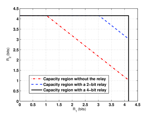
Figure 5: Capacity region of the Gaussian Z-interference channel in the strong interference regime with and without a digital relay link of Type I.

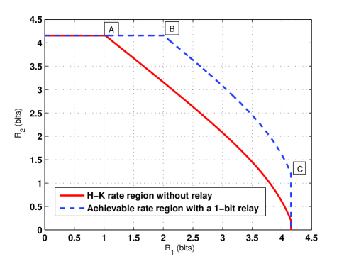
Figure 6: Achievable rate region of the Gaussian Z-interference channel in the weak interference regime with and without a digital relay link of Type I.

In the weak interference regime, the achievable rate region in Theorem 1 is obtained by a Han-Kobayashi common-private power splitting scheme. By inspection, the effect of a relay link is to shift the rate region curve upward by $R_{0}$ bits while limiting $R_{2}$ by its single-user bound $\gamma(\mathsf{SNR}_{2})$. Interestingly, although the relay link of rate $R_{0}$ is provided from receiver $2$ to receiver $1$, it can help $R_{2}$ by exactly $R_{0}$ bits, while it can only help $R_{1}$ by strictly less than $R_{0}$ bits. As a numerical example, Fig. 6 shows the achievable rate region of a Gaussian Z-interference channel with $\mathsf{SNR}_{1}=\mathsf{SNR}_{2}=25$dB and $\mathsf{INR}_{2}=20$dB. The solid curve represents the rate region achieved without the relay link. The dashed rate region is with a relay of rate $R_{0}=1$ bit. For most part of the curve, $R_{0}$ provides a 1-bit increase in $R_{2}$, but a less than 1-bit increase in $R_{1}$.

It is illustrative to identify the correspondence between the various points in the rate region and the different common-private splittings in the weak interference regime. Point $A$ corresponds to $\beta=1$. This is where the entire $X_{2}$ is private message. In this case, it is easy to verify that the first term of $R_{2}$ in (2) is less than the second term:

$$\gamma(\mathsf{SNR}_{2})<\gamma(\beta\mathsf{SNR}_{2})+\gamma\left(\frac{\overline{\beta}\mathsf{INR}_{2}}{1+\mathsf{SNR}_{1}+\beta\mathsf{INR}_{2}}\right)+R_{0}$$ (13)

As $\beta$ decreases, more private message is converted into common message, which means that less interference is seen at receiver $1$. As a result, $R_{1}$ increases, $R_{2}$ is kept at a constant (since (13) continues to hold). Graphically, as $\beta$ decreases from $1$, the achievable rate pair moves horizontally from point $A$ to the right until it reaches point $B$, corresponding to some $\beta^{*}$, after which the second term of $R_{2}$ in (2) becomes less than the first term $\gamma(\mathsf{SNR}_{2})$. The value of $\beta^{*}$ can be computed as

$$\beta^{*}=\frac{(1+\mathsf{SNR}_{1})(1+\mathsf{SNR}_{2})-2^{2R_{0}}(1+\mathsf{SNR}_{1}+\mathsf{INR}_{2})}{2^{2R_{0}}\mathsf{SNR}_{2}(1+\mathsf{SNR}_{1}+\mathsf{INR}_{2})-\mathsf{INR}_{2}(1+\mathsf{SNR}_{2})}.$$ (14)

As $\beta$ decreases further from $\beta^{*}$, more private message is converted into common message, which makes $R_{1}$ even larger. However, when $\beta<\beta^{*}$, the amount of common message can be transmitted is restricted by the interference link $h_{21}$ and the digital link rather than the direct link $h_{22}$. Therefore, user $2$’s data rate cannot be kept as a constant; $R_{2}$ goes down as user $1$’s rate goes up. As shown in Fig. 6, the achievable rate pair moves from point $B$ to point $C$ as $\beta$ decreases from $\beta^{*}$ to $0$. Point $C$ corresponds to where the entire $X_{2}$ is common message.

II-D Asymptotic Sum Capacity

Practical communication systems often operate in the interference-limited regime, where both the signal and the interference are much stronger than noise. In this section, we investigate the asymptotic sum capacity of the Type I Gaussian Z-relay-interference channel in the weak interference regime where noise power $N\rightarrow 0$, while power constraints $P_{1}$, $P_{2}$, channel gains $h_{ij}$, and the digital relay link rate $R_{0}$ are kept fixed. In other words, $\mathsf{SNR}_{1},\mathsf{SNR}_{2},\mathsf{INR_{2}}\rightarrow\infty$, while their ratios are kept constant.

Denote the sum capacity of a Type I Gaussian Z-interference channel with a relay link of rate $R_{0}$ by $C_{sum}(R_{0})$. Without the digital relay link, or equivalently $R_{0}=0$, the sum capacity of the classic Gaussian Z-interference channel in the weak interference regime (i.e. $\mathsf{INR_{2}\leq SNR_{2}}$) is given by [9, 5]:

$$C_{sum}(0)=\gamma(\mathsf{SNR}_{2})+\gamma\left(\frac{\mathsf{SNR}_{1}}{1+\mathsf{INR}_{2}}\right),$$ (15)

which is achieved by independent Gaussian codebooks and treating the interference as noise at the receiver. In the high SNR/INR limit, the above sum capacity becomes

$$C_{sum}(0)\approx\frac{1}{2}\log\left(\frac{\mathsf{SNR_{2}}(\mathsf{SNR_{1}+INR_{2}})}{\mathsf{INR}_{2}}\right),$$ (16)

where the notation $f(x)\approx g(x)$ is used to denote $\lim f(x)-g(x)=0$. In the above expression, the limit is taken as $N\rightarrow 0$.

Intuitively, with a digital relay link of finite capacity $R_{0}$, the sum-rate increase due to the relay must be bounded by $R_{0}$. The following theorem shows that in the high SNR/INR limit, the asymptotic sum-capacity increase is in fact $R_{0}$ in the weak-interference regime.

Theorem 2

For the Type I Gaussian Z-interference channel with a digital relay link of limited rate $R_{0}$ from the interference-free receiver to the interfered receiver as shown in Fig. 1(a), when $\mathsf{INR_{2}}\leq\mathsf{\min\{SNR_{2},INR_{2}^{*}\}}$, the asymptotic sum capacity is given by

$$C_{sum}(R_{0})\approx C_{sum}(0)+R_{0}.$$ (17)

Proof:

We first prove the achievability. As illustrated in Fig. 3 the sum rate of the Type I Gaussian Z-relay-interference channel is achieved with $\beta=\beta^{*}$, where $\beta^{*}$ is as derived in (14). In the high SNR/INR limit, we have

$$\lim_{N\rightarrow 0}\beta^{*}=\frac{2^{-2R_{0}}}{1+(1-2^{-2R_{0}})\frac{\mathsf{INR_{2}}}{\mathsf{SNR_{1}}}}.$$ (18)

Substituting this $\beta^{*}$ into the achievable rate pair in (2), we obtain the asymptotic rate pair as

$$\left\{\begin{array}[]{l}\displaystyle R_{1}\approx\frac{1}{2}\log\left(1+\frac{\mathsf{SNR_{1}}}{\mathsf{INR_{2}}}\right)+R_{0}\\ \displaystyle R_{2}\approx\frac{1}{2}\log(\mathsf{SNR_{2}})\end{array}\right.$$ (19)

which gives the following asymptotic sum rate:

$$R_{sum} \approx \frac{1}{2}\log\left(\frac{\mathsf{SNR_{2}}(\mathsf{SNR_{1}+INR_{2}})}{\mathsf{INR}_{2}}\right)+R_{0}$$ (20)

$$\approx C_{sum}(0)+R_{0}.$$

The converse proof starts with Fano’s inequality. Denote the output of the digital relay link over the $n$-block by $V^{n}$. Since the digital link has a capacity limit $R_{0}$, $V^{n}$ is a discrete random variable with $H(V^{n})\leq nR_{0}$. For a codebook of block length $n$, we have

$$n(R_{1}+R_{2})$$ (21)

$$\leq I(X_{1}^{n};Y_{1}^{n},V^{n})+I(X_{2}^{n};Y_{2}^{n})+n\epsilon_{n}$$

$$= I(X_{1}^{n};Y_{1}^{n})+I(X_{1}^{n};V^{n}|Y_{1}^{n})+I(X_{2}^{n};Y_{2}^{n})+n\epsilon_{n}$$

$${\leq} I(X_{1}^{n};Y_{1}^{n})+H(V^{n}|Y_{1}^{n})+I(X_{2}^{n};Y_{2}^{n})+n\epsilon_{n}$$

$${\leq} I(X_{1}^{n};Y_{1}^{n})+I(X_{2}^{n};Y_{2}^{n})+nR_{0}+n\epsilon_{n}$$

$${\leq} nC_{sum}(0)+nR_{0}+n\epsilon_{n},$$

where $\epsilon_{n}\rightarrow 0$ as $n$ goes to infinity. Note that this upper bound holds for all ranges of $\mathsf{SNR_{1}}$, $\mathsf{SNR_{2}}$, and $\mathsf{INR_{2}}$. This, when combined with the asymptotic achievability result proved earlier, gives the asymptotic sum capacity $C_{sum}(R_{0})\approx C_{sum}(0)+R_{0}$. ∎

The above proof focuses on the sum-capacity achieving power splitting ratio $\beta^{*}$. As $\beta\leq\beta^{*}$, the achievable rate pair goes from point $B$ to point $C$ along the dashed curve as shown in Fig. 6. It turns out that for any fixed $0<\beta\leq\beta^{*}$, the sum rate also asymptotically approaches the upper bound, thus providing an alternative proof for Theorem 2.

To see this, fix some arbitrary $0<\beta\leq\beta^{*}$, the sum rate corresponding to this $\beta$ is given in Theorem 1 as

$$R_{sum} = \gamma\left(\frac{\mathsf{SNR}_{1}}{1+\beta\mathsf{INR}_{2}}\right)+\gamma(\beta\mathsf{SNR}_{2})+$$ (22)

$$\qquad\gamma\left(\frac{\overline{\beta}\mathsf{INR}_{2}}{1+\mathsf{SNR}_{1}+\beta\mathsf{INR}_{2}}\right)+R_{0}$$

$$= \frac{1}{2}\log\left(\mathsf{\frac{1+\beta SNR_{2}}{1+\beta INR_{2}}}\right)+\gamma(\mathsf{SNR_{1}+INR_{2}})+R_{0}$$

$$\approx \frac{1}{2}\log\left(\frac{\mathsf{SNR_{2}}(\mathsf{SNR_{1}+INR_{2}})}{\mathsf{INR}_{2}}\right)+R_{0},$$

which is the asymptotic sum capacity. This calculation implies that in the high SNR/INR regime, the dashed curve in Fig. 6 has an initial slope of -1 as $\beta$ goes from $\beta^{*}$ to $0$.

Interestingly, decode-and-forward is not the only way to asymptotically achieve the sum capacity of the Type I channel. The following shows that a compress-and-forward relaying scheme, although strictly suboptimal in finite SNR/INR, becomes asymptotically sum-capacity achieving in the high SNR/INR limit in the weak interference regime, thus giving yet another proof of Theorem 2.

In the compress-and-forward scheme, no common-private power splitting is performed. Each receiver only decodes the message intended for it. Specifically, receiver $2$ compresses its received signal $Y_{2}$ into $\hat{Y}_{2}$, then forwards it to receiver $1$ through the digital link $R_{0}$.

Clearly, the rate of user $2$ is given by

$$R_{2}=\max_{p(x_{2})}I(X_{2};Y_{2}).$$ (23)

Using the Wyner-Ziv coding strategy [28, 10], for a fixed $p(x_{2})$, the following rate for user $1$ is achievable:

$$R_{1}=\max_{p(x_{1})p(\hat{y}_{2}|y_{2})}I(X_{1};Y_{1},\hat{Y}_{2})$$ (24)

under the constraint

$$I(Y_{2};\hat{Y}_{2}|Y_{1})\leq R_{0}.$$ (25)

The optimization in (24) is in general hard. Here, we adopt independent Gaussian codebooks with $X_{1}\sim\mathcal{N}(0,P_{1})$ and $X_{2}\sim\mathcal{N}(0,P_{2})$, and a Gaussian quantization scheme for the compression of $Y_{2}$:

$$\hat{Y}_{2}=Y_{2}+e$$ (26)

where $e$ is a Gaussian random variable independent of $Y_{2}$, with a distribution $\mathcal{N}(0,\sigma^{2})$. We show in Appendix -C that this choice of $p(x_{1})p(x_{2})p(\hat{y}_{2}|y_{2})$ gives the following achievable rate pair:

$$\left\{\begin{array}[]{l}\displaystyle R_{1}=\gamma\left(\frac{\mathsf{SNR_{1}}}{1+\mathsf{INR_{2}}}\right)+R_{0}-\delta_{0}(R_{0})\\ \displaystyle R_{2}=\gamma(\mathsf{SNR_{2}})\end{array}\right.$$ (27)

where

$$\delta_{0}(R_{0})=$$

$$\gamma\left(\frac{(2^{2R_{0}}-1)(1+\mathsf{SNR_{2}}+\mathsf{INR_{2}})(1+\mathsf{SNR_{1}}+\mathsf{INR_{2}})}{(\mathsf{1+INR_{2}})(\mathsf{(1+SNR_{1})(1+SNR_{2})+INR_{2}})}\right).$$

Let $N\rightarrow 0$, the above rate pair asymptotically goes to

$$\left\{\begin{array}[]{l}\displaystyle R_{1}\approx\frac{1}{2}\log\left(1+\frac{\mathsf{SNR_{1}}}{\mathsf{INR_{2}}}\right)+R_{0}\\ R_{2}\approx\frac{1}{2}\log(\mathsf{SNR_{2}})\end{array}\right.$$ (28)

which again achieves the asymptotic sum capacity (17). We remark that this is akin to the capacity result for a class deterministic relay channel [11], where both decode-and-forward and compress-and-forward are shown to be capacity achieving.

Although we have demonstrated the asymptotic sum-rate optimality of the point $B$ and all points between $B$ and $C$ in the weak interference regime as $N\rightarrow 0$ (while the ratios of SNRs and INRs are kept fixed), we remark that the achievable region (2) may not be asymptotically optimal in other regimes. For example, in the regime where $\mathsf{SNR}_{2}\gg\mathsf{INR}_{2}$, both the $R_{1}+R_{2}$ and $2R_{1}+R_{2}$ values at point $C$ ($\beta=0$) are unbounded away from their corresponding upper bounds as shown by Wang and Tse [21, Lemma 5.1] (Eq. (22) and Eq. (26)). To close this gap, one can use Wang and Tse’s quantize-map-and-forward approach [21], which in fact achieves the capacity region of the general Gaussian interference channel with bidirectional links to within a constant number of bits.

III Gaussian Z-Interference Channel with
a Relay Link: Type II

III-A Achievable Rate Region

As a counterpart of the Type I channel considered in the previous section, this section studies the Type II channel, where the relay link goes from the interfered receiver to the interference-free receiver as shown in Fig. 1(b). Intuitively, when the interference link is weak, the digital link would not be as efficient as in the Type I channel, because receiver $1$’s knowledge of $X_{2}$ is inferior to that of the receiver $2$. However, when the interference link is very strong, receiver $1$ becomes a better receiver for $X_{2}$ than receiver $2$, in which case the digital link is capable of increasing user $2$’s rate by as much as $R_{0}$.

The main difference between the Type I and the Type II channels is that in the Type I channel, the relay ($Y_{2}$) observes a noisy version of the interference at the relay destination ($Y_{1}$). In addition, the interference consists of messages intended for $Y_{2}$. Thus, the decoding and the forwarding of the interference is a natural strategy. In the Type II channel, the relay ($Y_{1}$) observes a noisy version of the intended signal at the relay destination ($Y_{2}$). Thus, decode-and-forward and compress-and-forward can both be used. The following achievability theorem is based on a combination of the Han-Kobayashi scheme (with $\beta$ being the common-private splitting ratio) and two relay strategies, where the relay decodes then forwards the common information using a rate $R_{a}$ and compresses then forwards the private information using a rate $R_{b}$, with $R_{a}+R_{b}=R_{0}$, as shown in Fig. 7. In addition, the presence of common information gives rise to the possibility of compressing a combination of private and common messages. A parameter $\alpha$ accounts for the combination of private and common message compression.

Unlike the Type I channel, the achievable rate region for the Type II Gaussian Z-relay-interference channel has a more complicated structure. In addition to the weak, strong and very strong interference regimes, there is a new moderately strong regime, where a combination of the decode-and-forward and the compress-and-forward strategies is proposed. The proposed scheme reduces to pure compress-and-forward in the weak interference regime, and pure decode-and-forward in the strong interference regime.

\psfrag{X1}{$X_{1}$}\psfrag{X2}{$X_{2}$}\psfrag{Y1}{$Y_{1}$}\psfrag{Y2}{$Y_{2}$}\psfrag{U2}{$U_{2}$}\psfrag{W2}{$W_{2}$}\psfrag{Z1}{$Z_{1}$}\psfrag{Z2}{$Z_{2}$}\psfrag{R0}{$R_{0}$}\psfrag{S1}{$S_{1}$}\psfrag{T2}{$T_{2}$}\psfrag{S2}{$S_{2}$}\psfrag{P1}{$P_{1}$}\psfrag{b_P2}{$\overline{\beta}P_{2}$}\psfrag{bP2}{$\beta P_{2}$}\psfrag{h11}{$h_{11}$}\psfrag{h22}{$h_{22}$}\psfrag{h21}{$h_{21}$}\includegraphics[width=238.49121pt]{./figures/hk_relay_ic_type_ii}

Figure 7: Common-private power splitting for Type II channel with $R_{0}=R_{a}+R_{b}$, where $R_{a}$ is used to decode-and-forward $W_{2}$, and $R_{b}$ is used to compress-and-forward $U_{2}$.

Theorem 3

For the Type II Gaussian Z-interference channel with a digital relay link of limited rate $R_{0}$ from the interfered receiver to the interference-free receiver as shown in Fig. 1(b), in the weak interference regime defined by $\mathsf{INR_{2}\leq SNR_{2}}$, the following rate region is achievable:

$$\bigcup_{0\leq\beta\leq 1}\left\{(R_{1},R_{2})\left|R_{1}\leq\gamma\left(\frac{\mathsf{SNR}_{1}}{1+\beta\mathsf{INR}_{2}}\right),\right.\right.\\ R_{2}\leq\gamma(\mathsf{\beta SNR_{2}})+\left.\gamma\left(\mathsf{\frac{\overline{\beta}INR_{2}}{1+SNR_{1}+\beta INR_{2}}}\right)+\delta(\beta,R_{0})\right\},$$ (29)

where

$$\delta(\beta,R_{0})=\gamma\left(\frac{\beta(2^{2R_{0}}-1)\mathsf{INR_{2}}}{2^{2R_{0}}(\mathsf{1+\beta SNR_{2}})+\mathsf{\beta INR_{2}}}\right).$$ (30)

In the moderately strong interference regime, defined by

$$\mathsf{SNR_{2}\leq INR_{2}}\leq 2^{2R_{0}}(1+\mathsf{SNR_{2}})-1\stackrel{{\scriptstyle\bigtriangleup}}{{=}}\mathsf{INR}_{2}^{\dagger},$$ (31)

the following rate region is achievable:

$$\mathrm{co}\left\{\bigcup_{\alpha\in\mathbb{R},0\leq\beta\leq 1,\;R_{a}+R_{b}\leq R_{0}}\mathcal{R}_{\alpha,\beta}(R_{a},R_{b})\right\},$$ (32)

where “co” denotes convex hull and $\mathcal{R}_{\alpha,\beta}(R_{a},R_{b})$ is a pentagon region given by

$$\left\{(R_{1},R_{2})\left|\begin{array}[]{l}R_{1}\leq\gamma(\mathsf{\frac{SNR_{1}}{1+\beta INR_{2}}})\\ R_{2}\leq\min\left\{\gamma(\mathsf{SNR_{2}})+R_{b}+\eta(\alpha,\beta,R_{a}),\right.\\ \qquad\qquad\quad\gamma(\mathsf{\beta SNR_{2}})+\gamma\left(\mathsf{\frac{\overline{\beta}INR_{2}}{1+\beta INR_{2}}}\right)\\ \qquad\qquad\quad\left.+\zeta(\alpha,\beta,R_{a})\right\}\\ R_{1}+R_{2}\leq\gamma(\beta\mathsf{SNR_{2}})+\gamma\left(\mathsf{\frac{SNR_{1}+\overline{\beta}INR_{2}}{1+\beta INR_{2}}}\right)\\ \qquad\qquad\quad+\zeta(\alpha,\beta,R_{a})\end{array}\right.\right\},$$ (33)

where

$$\zeta(\alpha,\beta,R_{a})=\gamma\left(\frac{\beta\mathsf{INR_{2}}}{(1+\beta\mathsf{SNR_{2}})(1+\frac{\sigma^{2}}{N})}\right),$$ (34)

and

$$\eta(\alpha,\beta,R_{a})=\\ \gamma\left(\frac{(1+2\alpha\overline{\beta}+\alpha^{2}\overline{\beta})\mathsf{INR_{2}}+\beta\overline{\beta}\alpha^{2}\mathsf{INR_{2}}\mathsf{SNR_{2}}}{(1+\mathsf{SNR_{2}})(1+\frac{\sigma^{2}}{N})}\right)$$ (35)

with

$$\frac{\sigma^{2}}{N}=\frac{1+\mathsf{SNR_{2}}+(1+2\alpha\overline{\beta}+\alpha^{2}\overline{\beta})\mathsf{INR_{2}}+\beta\overline{\beta}\alpha^{2}\mathsf{INR_{2}}\mathsf{SNR_{2}}}{(2^{2R_{a}}-1)(1+\mathsf{SNR_{2}})}.$$ (36)

In the strong interference regime defined by

$$\mathsf{INR}_{2}^{\dagger}\leq\mathsf{INR_{2}}\leq\mathsf{(1+SNR_{1})}\mathsf{INR}_{2}^{\dagger}\stackrel{{\scriptstyle\bigtriangleup}}{{=}}\mathsf{INR}_{2}^{{\ddagger}},$$ (37)

the capacity region is given by

$$\left\{(R_{1},R_{2})\left|\begin{array}[]{rll}R_{1}&\leq&\gamma(\mathsf{SNR_{1}})\\ R_{2}&\leq&\gamma(\mathsf{SNR_{2}})+R_{0}\\ R_{1}+R_{2}&\leq&\gamma(\mathsf{SNR_{1}+INR_{2}})\end{array}\right.\right\}.$$ (38)

In the very strong interference regime defined by

$$\mathsf{INR_{2}}\geq\mathsf{INR}_{2}^{{\ddagger}},$$ (39)

the capacity region is given by

$$\left\{(R_{1},R_{2})\left|\begin{array}[]{l}R_{1}\leq\gamma(\mathsf{SNR_{1}})\\ R_{2}\leq\gamma(\mathsf{SNR_{2}})+R_{0}\end{array}\right.\right\}.$$ (40)

Proof:

See Appendix -D. ∎

III-B Numerical Examples

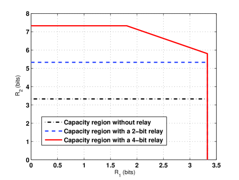
Figure 8: Achievable region of the Gaussian Z-interference channel in the strong interference regime with and without a digital relay link of Type II.

In the strong and very strong interference regimes, the entire $X_{2}$ is common information. The relay expands the capacity region by decoding $X_{2}^{n}$ at receiver $1$ and forwarding its bin index to receiver $2$. The boundaries of the strong and very strong regimes depend on the relay link rate. As a numerical example, Fig. 8 shows how the capacity region of a Type II channel is expanded by the relay link in the strong and very strong interference regimes. Here, $\mathsf{SNR_{1}=SNR_{2}=20}$ dB and $\mathsf{INR_{2}=55}$ dB. Without the digital link, this is a Gaussian Z-interference channel in the very strong interference regime [8], where $\mathsf{INR_{2}\geq SNR_{2}(1+SNR_{1})}$ and the capacity region is a rectangle as depicted by the dash-dotted region in Fig. 8. With a 2-bit digital link, $R_{2}$ is expanded by exactly 2 bits. The Z-interference channel remains in the very strong interference regime, where the capacity region is given by (40) and depicted by the dashed rectangular region in Fig. 8. When $R_{0}=4$ bits, the Z-interference channel now falls into the strong interference regime. The capacity region as given by (38) now becomes a solid pentagon region. Further increase in the rate of the digital link can increase the maximum $R_{2}$ but not the sum rate.

In the weak interference regime where $\mathsf{INR_{2}\leq SNR_{2}}$, Theorem 3 shows that a pure compress-and-forward for the private message should be used for relaying. Intuitively, this is because when the interference link is weak the common message rate is limited by the interference link, which cannot be helped by relaying. Thus, the digital link needs to focus on helping the decoding of private message at $Y_{2}$ by compress-and-forward. As a numerical example, Fig. 9 shows the achievable rate region of a Gaussian Z-interference channel with $\mathsf{SNR_{1}=SNR_{2}=20}$ dB and $\mathsf{INR_{2}=15}$ dB with and without the relay link. The dashed region denoted by points $A^{\prime}$ and $B$ represents the rate region achieved without the digital link. The solid rate region denoted by points $A$ and $B$ is with a 2-bit digital link. From the rate pair expression (29), the effect of the digital link is to shift the rate region of the channel without the relay upward by $\delta(\beta,R_{0})$ bits. Since $\delta(\beta,R_{0})$ is monotonically decreasing as $\beta$ decreases from 1 to 0, for fixed $R_{1}$, the largest increase in $R_{2}$ corresponds to $\delta(1,R_{0})$, i.e. the increase from point $A^{\prime}$ to $A$. Note that $A$ and $A^{\prime}$ are the maximum sum-rate points of the Type II Gaussian Z-interference channel with and without the relay respectively. They correspond to all-private message transmission, which is in contrast to the Type I case where the maximum sum rate is achieved with some $\beta^{*}\neq 1$. Finally, we note that the relay does not affect point $B$, which corresponds to $\beta=0$, because $\delta(0,R_{0})=0$.

\begin{overpic}[scale={0.6}]{./figures/Z_weak_qtz_typeII.eps} \centering\put(35.0,63.0){\small$A$} \put(33.0,55.0){\small$A^{\prime}$} \put(87.0,11.0){\small$B$} \@add@centering\end{overpic}

Figure 9: Capacity region of the Gaussian Z-interference channel in the weak interference regime with and without a digital relay link of Type II.

III-C Sum-Capacity Upper Bound

By Theorem 3, an achievable sum rate of the Type II Gaussian Z-interference channel with a relay link of rate $R_{0}$ in the weak interference regime is

$$R_{sum}=\gamma\left(\frac{\mathsf{SNR}_{1}}{1+\mathsf{INR}_{2}}\right)+\gamma(\mathsf{SNR_{2}})+\delta(1,R_{0}),$$ (41)

which is obtained by setting $\beta=1$ in (29). Comparing with the sum capacity of the Gaussian Z-interference channel without the relay in the weak interference regime (15), the sum-rate increase using the relay scheme of Theorem 3 is upper bounded by

$$\delta(1,R_{0}) = \frac{1}{2}\log\left(\frac{\mathsf{1+SNR_{2}+INR_{2}}}{\mathsf{1+SNR_{2}}+2^{-2R_{0}}\mathsf{INR_{2}}}\right)$$ (42)

$$\leq \gamma\left(\frac{\mathsf{INR_{2}}}{\mathsf{1+SNR_{2}}}\right)$$

$$\leq \frac{1}{2},$$

where $\mathsf{INR_{2}\leq SNR_{2}}$ is used in the last step. As illustrated in the example in Fig. 9, the rate increase from point $A^{\prime}$ to point $A$ is about 0.2 bits, which is less than 1/2 bits and is a fraction of the 2-bit relay link rate. This is in contrast to the Type I channel, where each relay bit can increase the sum rate by up to one bit. The following theorem provides an asymptotic sum-capacity result for the Type II channel and a proof of the 1/2-bit upper bound when $\mathsf{INR_{2}}$ is not very strong.

Theorem 4

For the Type II Gaussian Z-interference channel with a digital relay link of rate $R_{0}$ from the interfered receiver to the interference-free receiver as shown in Fig. 1(b), when $R_{0}\rightarrow\infty$, the asymptotic sum capacity is

$$C_{sum}(\infty)=\gamma(\mathsf{SNR_{1}+INR_{2}})+\gamma\left(\mathsf{\frac{SNR_{2}}{1+INR_{2}}}\right).$$ (43)

Further, when $\mathsf{INR_{2}\leq INR_{2}^{\S}}$, where $\mathsf{INR_{2}^{\S}}$ is defined by $\mathsf{INR_{2}^{\S}=SNR_{2}(1+SINR_{1})}$, we have

$$C_{sum}(\infty)-C_{sum}(0)\leq\frac{1}{2}.$$ (44)

Proof:

When $R_{0}=\infty$, receiver $2$ has complete knowledge of $Y_{1}^{n}$. Starting from Fano’s inequality:

$$n(R_{1}+R_{2})$$ (45)

$$\leq I(X_{1}^{n};Y_{1}^{n})+I(X_{2}^{n};Y_{1}^{n},Y_{2}^{n})+n\epsilon_{n}$$

$$\stackrel{{\scriptstyle(a)}}{{\leq}} I(X_{1}^{n};Y_{1}^{n})+I(X_{2}^{n};Y_{1}^{n},Y_{2}^{n}|X_{1}^{n})+n\epsilon_{n}$$

$$= I(X_{1}^{n},X_{2}^{n};Y_{1}^{n})+I(X_{2}^{n};Y_{2}^{n}|Y_{1}^{n},X_{1}^{n})+n\epsilon_{n},$$

where (a) follows from the fact that $X_{1}^{n}$ is independent of $X_{2}^{n}$. The first term in (45) is bounded by the sum capacity of the multiple-access channel $(X_{1}^{n},X_{2}^{n},Y_{1}^{n})$:

$$I(X_{1}^{n},X_{2}^{n};Y_{1}^{n})\leq n\gamma(\mathsf{SNR_{1}+INR_{2}})$$ (46)

The second term in (45) is bounded by

$$I(X_{2}^{n};Y_{2}^{n}|Y_{1}^{n},X_{1}^{n})$$ (47)

$$= h(Y_{2}^{n}|Y_{1}^{n},X_{1}^{n})-h(Y_{2}^{n}|Y_{1}^{n},X_{1}^{n},X_{2}^{n})$$

$$\stackrel{{\scriptstyle(a)}}{{\leq}} \sum_{i=1}^{n}\left\{h(Y_{2,i}|Y_{1,i},X_{1,i})-h(Z_{2,i})\right\}$$

$$= \sum_{i=1}^{n}\left\{h(h_{22}X_{2,i}+Z_{2,i}|h_{21}X_{2,i}+Z_{1,i})-h(Z_{2,i})\right\}$$

$$\stackrel{{\scriptstyle(b)}}{{\leq}} n\gamma\left(\mathsf{\frac{SNR_{2}}{1+INR_{2}}}\right),$$

where (a) follows from the chain rule and the fact that conditioning does not increase entropy, and (b) follows from the fact that Gaussian distribution maximizes the conditional entropy under a covariance constraint. Combining (46) and (47) gives the sum rate upper bound:

$$C_{sum}(\infty)\leq\gamma(\mathsf{SNR_{1}+INR_{2}})+\gamma\left(\mathsf{\frac{SNR_{2}}{1+INR_{2}}}\right).$$ (48)

It can be easily verified that the above sum-rate upper bound is also asymptotically achievable. By Theorem 3, with $R_{0}=\infty$, there are only two interference regimes: weak interference regime and moderately strong interference regime. In the weak interference regime, a pure compress-and-forward scheme, i.e., setting $\beta=1$ in (29) achieves (48). In the moderately strong interference regime, setting $\beta=1$ and $R_{b}=0$ in (33) achieves

$$\gamma(\mathsf{SNR_{2}})+\gamma\left(\mathsf{\frac{SNR_{1}}{1+INR_{2}}}\right)+\gamma\left(\mathsf{\frac{INR_{2}}{1+SNR_{2}}}\right)$$ (49)

which is equivalent to (48). This proves the asymptotic sum-capacity result.

Now, without the relay link, the sum capacity for the Gaussian Z-interference channel is ([7, 8, 1, 9, 5]):

$$C_{sum}(0)=$$

$$\left\{\begin{array}[]{ll}\gamma(\mathsf{SNR_{2}})+\displaystyle\gamma\left(\mathsf{\frac{SNR_{1}}{1+INR_{2}}}\right)&\mathrm{if\ \ }\mathsf{INR_{2}\leq SNR_{2}}\\ \gamma(\mathsf{SNR_{1}+INR_{2}})&\mathrm{if\ \ }\mathsf{SNR_{2}\leq INR_{2}\leq INR_{2}^{\S}}\\ \gamma(\mathsf{SNR_{1}})+\gamma(\mathsf{SNR_{2}})&\mathrm{if\ \ }\mathsf{INR_{2}\geq INR_{2}^{\S}}\end{array}\right.$$

Comparing $C_{sum}(0)$ with the asymptotic sum capacity in the limit of large relay rate (43), we have

$$C_{sum}(\infty)-C(0)=\gamma\left(\mathsf{\frac{INR_{2}}{1+SNR_{2}}}\right)\leq\frac{1}{2}$$ (51)

when $\mathsf{INR_{2}\leq SNR_{2}}$ and

$$C_{sum}(\infty)-C(0)=\gamma\left(\mathsf{\frac{SNR_{2}}{1+INR_{2}}}\right)\leq\frac{1}{2}$$ (52)

when $\mathsf{SNR_{2}\leq INR_{2}\leq INR_{2}^{\S}}$. Therefore, the sum-capacity gain is upper bounded by half a bit when $\mathsf{INR_{2}\leq INR_{2}^{\S}}$. ∎

Note that when $\mathsf{INR_{2}\geq INR_{2}^{\S}}$, the sum-capacity gain can be larger than half a bit. In fact, in the regime where $\mathsf{INR_{2}\gg SNR_{1},INR_{2}\gg SNR_{2}}$ and $\mathsf{SNR_{1},SNR_{2}}\gg 1$, we have

$$C_{sum}(\infty)-C_{sum}(0)\approx\frac{1}{2}\log\left(\mathsf{\frac{INR_{2}}{SNR_{1}SNR_{2}}}\right),$$ (53)

which can be unbounded.

The asymptotic sum capacity (43) is essentially the sum capacity of a degraded Gaussian interference channel where the inputs are $X_{1}$ and $X_{2}$, and outputs are $Y_{1}$ and $(Y_{1},Y_{2})$ of a Gaussian Z-interference channel. The capacity region for the general degraded interference channel is still open.

IV Summary

This paper studies a Gaussian Z-interference channel with unidirectional relay link at the receiver. When the relay link goes from the interference-free receiver to the interfered receiver, a suitable relay strategy is to let the interference-free receiver decode-and-forward a part of the interference for subtraction. Interference decode-and-forward is capacity achieving in the strong interference regime. In the weak interference regime, the asymptotic sum capacity can be achieved with either a decode-and-forward or a compress-and-forward strategy in the high SNR/INR limit.

When the relay link goes from the interfered receiver to the interference-free receiver, a suitable relay strategy is a combination of decode- and compress-and-forward of the intended message. In the strong interference regime, decode-and-forward alone is capacity achieving. In the weak interference regime, the combination scheme reduces to pure compress-and-forward. In the moderately strong interference regime, a combination of both need to be used.

The direction of the relay link is crucial. In the weak interference regime, a relay link from the interference-free receiver to the interfered receiver can significantly increase the achievable sum rate by up to one bit for every relay bit, while in the reversed direction, the sum rate increase is upper bounded by half a bit regardless of the relay link rate. In contrast, in the strong interference regime, the sum-capacity gain due to a relay from the interference-free receiver to the interfered receiver eventually saturates, while a relay link in the reverse direction provides unbounded sum-capacity gain.

-A Convexity of Achievable Rate Region (9)

This appendix shows that the region defined by $R_{1}\leq\mathsf{\gamma(SNR_{1})}$, $R_{2}\leq\mathsf{\gamma(SNR_{2})}+R_{0}$, and the curve

$$\left\{\begin{array}[]{lll}R_{1}&=&\gamma\left(\displaystyle\frac{\mathsf{SNR}_{1}}{1+\beta\mathsf{INR}_{2}}\right)\\ R_{2}&=&\gamma(\beta\mathsf{SNR}_{2})+\gamma\left(\displaystyle\frac{\overline{\beta}\mathsf{INR}_{2}}{1+\mathsf{SNR}_{1}+\beta\mathsf{INR}_{2}}\right)+R_{0}\end{array}\right.$$ (54)

where $0\leq\beta\leq 1$, is convex when $\mathsf{INR_{2}\leq SNR_{2}}$.

Note that, when $\beta=1$ and $\beta=0$, the curve defined by (54) meets $R_{2}=\mathsf{\gamma(SNR_{2})}+R_{0}$ and $R_{1}=\mathsf{\gamma(SNR_{1})}$ at points $A$ and $B$, respectively, as shown in Fig. 10. Therefore, to prove the convexity of the region, we only need to prove that the curve (54) parameterized by $\beta$ is concave.

Figure 10: The region defined by lines $R_{1}=\mathsf{\gamma(SNR_{1})}$, $R_{2}=\mathsf{\gamma(SNR_{2})}+R_{0}$ and the curve (54).

First, we express $\beta$ in terms of $R_{1}$:

$$\beta=\frac{1}{\mathsf{INR_{2}}}\left(\frac{\mathsf{SNR_{1}}}{2^{2R_{1}}-1}-1\right).$$ (55)

Substituting this expression for $\beta$ into the expression for $R_{2}$ in (54), we obtain $R_{2}$ as a function of $R_{1}$:

$$R_{2}=\frac{1}{2}\log\left(-\nu 2^{2R_{1}}+\lambda\right)+\mu$$ (56)

where $\nu=\mathsf{\frac{SNR_{2}}{INR_{2}}}-1$, $\lambda=\mathsf{\frac{SNR_{2}}{INR_{2}}(1+SNR_{1})}-1$ and $\mu=\gamma\left(\mathsf{\frac{1+INR_{2}}{SNR_{1}}}\right)+R_{0}$. Note that when $\mathsf{INR_{2}\leq SNR_{2}}$, $\nu\geq 0$ and $\lambda>0$.

Observe that $R_{1}$ is a monotonic decreasing function of $\beta$. So, in the range $0\leq\beta\leq 1$, we have

$$\gamma\left(\mathsf{\frac{SNR_{1}}{1+INR_{2}}}\right)\leq R_{1}\leq\gamma(\mathsf{SNR_{1}}).$$ (57)

In this range of $R_{1}$, it is easy to verify that $-\nu 2^{2R_{1}}+\lambda>0$.

Now, taking the first and second order derivatives of $R_{2}$ with respect to $R_{1}$ in (56), we have

$$R_{2}^{\prime}=\frac{-\nu 2^{2R_{1}}}{-\nu 2^{2R_{1}}+\lambda},\;\;\;\;R_{2}^{\prime\prime}=\frac{-2\lambda\nu 2^{2R_{1}}}{(-\nu 2^{2R_{1}}+\lambda)^{2}}\ln 2.$$ (58)

Since $\nu\geq 0$, $\lambda>0$, and $-\nu 2^{2R_{1}}+\lambda>0$, we have $R_{2}^{\prime}\leq 0$ and $R_{2}^{\prime\prime}\leq 0$. As a result, the curve (54) parameterized by $\beta$ is concave.

-B Converse Proof for the Strong and Very Strong Interference Regimes in Theorem 1

In this appendix, we prove a converse in the strong and very strong interference regimes for the Type I channel. The converse is based on a technique used in [1] and [8] for proving the converse for the strong interference channel without the relay link. The idea is to show that when $\mathsf{INR_{2}\geq\min\{SNR_{2},INR_{2}^{*}\}}$, if a rate pair $(R_{1},R_{2})$ is achievable for the Gaussian Z-interference channel with a relay link, i.e., $X_{1}^{n}$ can be reliably decoded at receiver $1$ at rate $R_{1}$, and $X_{2}^{n}$ can be reliably decoded at receiver $2$ at rate $R_{2}$, then $X_{2}^{n}$ must also be decodable at the receiver $1$.

First, the reliable decoding of $X_{2}^{n}$ at receiver $2$ requires

$$R_{2}\leq\mathsf{\gamma(SNR_{2})}.$$ (59)

To show that $X_{2}^{n}$ is also decodable at receiver $1$ when $\mathsf{INR_{2}\geq\min\{SNR_{2},INR_{2}^{*}\}}$, consider the two cases $\mathsf{SNR_{2}\leq INR_{2}^{*}}$ and $\mathsf{SNR_{2}\geq INR_{2}^{*}}$ separately.

First, when $\mathsf{SNR_{2}\leq INR_{2}^{*}}$, we have $\mathsf{INR_{2}\geq SNR_{2}}$, or $h_{21}\geq h_{22}$. In this case, after $X_{1}^{n}$ is decoded at receiver $1$ (possibly with the help of the relay link), receiver $1$ may subtract $X_{1}^{n}$ from $Y_{1}^{n}$ then scale the resulting signal to obtain

$$Y_{1}^{{}^{\prime}n}=\frac{h_{22}}{h_{21}}(Y_{1}^{n}-h_{11}X_{1}^{n})=h_{22}X_{2}^{n}+\frac{h_{22}}{h_{21}}Z_{1}^{n}.$$ (60)

When $h_{21}\geq h_{22}$, the Gaussian noise $\frac{h_{22}}{h_{21}}Z_{1}^{n}$ in this effective channel has a smaller variance than the noise in $Y_{2}^{n}=h_{22}X_{2}^{n}+Z_{2}^{n}$. Since $X_{2}^{n}$ is reliably decodable at receiver $2$, $X_{2}^{n}$ must also be reliably decodable at receiver $1$.

When $\mathsf{SNR_{2}\geq INR_{2}^{*}}$, we have $\mathsf{INR_{2}\geq INR_{2}^{*}}$. In this case, since $X_{2}^{n}$ is reliably decoded at $Y_{2}$, with the perfect knowledge of $X_{2}^{n}$ at receiver $2$, $(X_{2}^{n},Y_{1}^{n},Y_{2}^{n})$ forms a deterministic relay channel [11] with $X_{2}^{n}$ as the input, $Y_{1}^{n}$ as the output and $Y_{2}^{n}$ as the deterministic relay. As a result, the following rate for $X_{2}^{n}$ can be supported:

$$R_{2}=\gamma\left(\mathsf{\frac{INR_{2}}{1+SNR_{1}}}\right)+R_{0}$$ (61)

Since $\mathsf{INR_{2}\geq INR_{2}^{*}}$, it is easy to verify that the above rate is always greater than the rate supported at the receiver $2$, i.e.,

$$\gamma\left(\mathsf{\frac{INR_{2}}{1+SNR_{1}}}\right)+R_{0}\geq\gamma(\mathsf{SNR_{2}}),$$ (62)

which implies that whenever $X_{2}^{n}$ is reliably decodable at $Y_{2}$, it is also reliably decodable at $Y_{1}$ with the help of the relay.

Now, because both $X_{1}^{n}$ and $X_{2}^{n}$ are always decodable at receiver $1$ in the strong interference regime, the achievable rate region of the Gaussian Z-interference channel with a digital relay link is included in the capacity region of the same channel in which both $X_{1}^{n}$ and $X_{2}^{n}$ are required at $Y_{1}^{n}$, and $X_{2}^{n}$ is required at $Y_{2}^{n}$. Further, the capacity region of such a channel can only be enlarged if $X_{2}^{n}$ is provided to $Y_{2}^{n}$ by a genie. In such a case, the channel reduces to a Gaussian multiple-access channel with $(X_{1}^{n},X_{2}^{n})$ as inputs, $Y_{1}^{n}$ as the output, and with the same relay link from receiver $2$ to receiver $1$, where the relay knows $X_{2}^{n}$ perfectly. The capacity region of such a channel is

$$\left\{(R_{1},R_{2})\left|\begin{array}[]{rll}R_{1}&\leq&\gamma(\mathsf{SNR_{1}})\\ R_{2}&\leq&\gamma(\mathsf{INR_{2}})+R_{0}\\ R_{1}+R_{2}&\leq&\gamma(\mathsf{SNR_{1}+INR_{2}})+R_{0}\end{array}\right.\right\}$$ (63)

Combining (63) and (59), then applying (11) gives us (4). This proves that when $\mathsf{INR_{2}\geq\min\{SNR_{2},INR_{2}^{*}\}}$, the achievable rate region of the Gaussian Z-interference channel with a relay link must be included in (4), which, in the very strong interference regime, reduces to (5).

-C Evaluation of Wyner-Ziv Rate (27)

In this appendix, we show that with independent Gaussian inputs $X_{1}\sim\mathcal{N}(0,P_{1})$ and $X_{2}\sim\mathcal{N}(0,P_{2})$, and the Gaussian quantization scheme (26), the achievable rate described by (23), (24) and (25) is given by (27). The technique is similar to that in [29].

With a Gaussian input $X_{2}\sim\mathcal{N}(0,P_{2})$, $R_{2}$ is given by

$$R_{2} = I(X_{2};Y_{2})=\gamma(\mathsf{SNR_{2}}).$$ (64)

With the knowledge of $X_{2}$ at $Y_{2}$, $X_{1}$, $Y_{1}$ together with $Y_{2}$ become a deterministic relay channel with a digital link. To fully utilize the digital link, we set $\hat{Y}_{2}$ to be such that $I(Y_{2};\hat{Y}_{2}|Y_{1})=R_{0}$. Note that $\hat{Y}_{2}=Y_{2}+e$, where $Y_{2}$ and $e$ are independent and $e\sim\mathcal{N}(0,\sigma^{2})$. To find $\sigma^{2}$, note that

$$R_{0}=h(\hat{Y}_{2}|Y_{1})-h(\hat{Y}_{2}|Y_{1},Y_{2})=\gamma\left(\frac{\sigma_{Y_{2}|Y_{1}}^{2}}{\sigma^{2}}\right)$$ (65)

where $\sigma_{Y_{2}|Y_{1}}^{2}$, the conditional variance of $Y_{2}$ given $Y_{1}$, can be calculated in a standard way. Thus, from (65), we have

$$\sigma^{2}=\frac{N}{2^{2R_{0}}-1}\left(1+\mathsf{\frac{SNR_{2}(1+SNR_{1})}{1+SNR_{1}+INR_{2}}}\right).$$ (66)

Now, we are ready to calculate $R_{1}$. First,

$$h(\hat{Y}_{2}|Y_{1},X_{1})$$ (67)

$$= \frac{1}{2}\log\left(2\pi e\left(\sigma^{2}+N\left(1+\mathsf{\frac{SNR_{2}}{1+INR_{2}}}\right)\right)\right)$$

where $\sigma^{2}$ is given by (66). Now, the rate of user $1$ is given by

$$R_{1} = I(X_{1};Y_{1},\hat{Y}_{2})$$ (68)

$$= I(X_{1};Y_{1})+h(\hat{Y}_{2}|Y_{1})-h(\hat{Y}_{2}|Y_{1},X_{1}).$$

Clearly, with independent Gaussian inputs $X_{1}\sim\mathcal{N}(0,P_{1})$ and $X_{2}\sim\mathcal{N}(0,P_{2})$,

$$I(X_{1};Y_{1})=\gamma\left(\mathsf{\frac{SNR_{1}}{1+INR_{2}}}\right).$$ (69)

Substituting (69), (67) and $h(\hat{Y}_{2}|Y_{1})$ from (65) into (68), after some calculations, we obtain $R_{1}$ in (27).

-D Proof of Theorem 3

We first prove the achievability of the rate region given in (32). We then show that (32) reduces to (29) in the weak interference regime, and reduces to (38) and (40) in the strong and very strong interference regimes, respectively.

A two-step decoding procedure is used to prove the achievability. Consider first the decoding of $(X_{1}^{n},W_{2}^{n})$ at $Y_{1}$. The achievable set of $(S_{1},T_{2})$ is the capacity region of a multiple-access channel, denoted by $\mathcal{C}_{1}$, which is just (7) with $R_{0}$ set to zero. Next, consider the decoding of $(W_{2}^{n},U_{2}^{n})$ at receiver $2$ with the help of a digital relay link of rate $R_{0}$. This is a multiple-access channel with a rate-limited relay, where the relay has complete knowledge of $W_{2}^{n}$ and a noisy observation $h_{21}U_{2}^{n}+Z_{1}^{n}$, obtained by subtracting $X_{1}^{n}$ and $W_{2}^{n}$ from the received signal at receiver $1$. Each of these two pieces of information is useful for decoding $(W_{2}^{n},U_{2}^{n})$ at receiver $2$.

Now, consider a relay scheme which splits the digital link in two parts: $R_{a}$ bits for describing $U_{2}^{n}$, and $R_{b}$ for describing $W_{2}$, where $R_{a}+R_{b}=R_{0}$. However, since only a noisy version of $U_{2}^{n}$ is available at the relay ($Y_{1}$), a compress-and-forward strategy using Wyner-Ziv coding ([28, 10]) may be used for describing $U_{2}^{n}$. One way to do compress-and-forward is to quantize $h_{21}U_{2}^{n}+Z_{1}^{n}$ with $Y_{2}^{n}$ acting as the decoder side information. However, the presence of $W_{2}^{n}$ offers other possibilities. First, receiver $2$ may choose to decode $W_{2}^{n}$ before decoding $U_{2}^{n}$, in which case $W_{2}^{n}$ becomes additional decoder side information for Wyner-Ziv coding. Second, instead of quantizing $h_{21}U_{2}^{n}+Z_{1}^{n}$ with $W_{2}^{n}$ completely subtracted from the relay’s observation, the relay may choose to subtract $W_{2}^{n}$ partially—doing so can benefit the Wyner-Ziv rate. This second approach is is adopted in the rest of the proof. Interestingly, the two approaches turn out to give identical achievable rates.

Specifically, let the relay form the following fictitious signal

$$\bar{Y}_{1}^{n}=h_{21}(U_{2}^{n}+W_{2}^{n})+\alpha h_{21}W_{2}^{n}+Z_{1}^{n}$$ (70)

for some $\alpha\in\mathbb{R}$. The proposed relay scheme, which combines the decode-and-forward technique and the compress-and-forward technique, is illustrated in Fig. 11, where $W_{2}^{n}$ and $U_{2}^{n}$ are the inputs of the multiple-access channel, $(Y_{2}^{n},\hat{Y}_{1}^{n})$ is the output, and $\hat{Y}_{1}^{n}$ is a quantized version of $\bar{Y}_{1}^{n}$. With complete knowledge of $W_{2}^{n}$ at the relay, the capacity of this multiple-access relay channel, denoted by $\mathcal{C}_{2}$, is given by the set of rates $(S_{2},T_{2})$ where

$$\left\{\begin{array}[]{rll}S_{2}&\leq&I(U_{2};Y_{2},\hat{Y}_{1}|W_{2})\\ T_{2}&\leq&I(W_{2};Y_{2},\hat{Y}_{1}|U_{2})+R_{b}\\ S_{2}+T_{2}&\leq&I(U_{2},W_{2};Y_{2},\hat{Y}_{1})+R_{b}\end{array}\right.$$ (71)

Similar to Theorem 1, we adopt $\bar{Y}_{1}$: $\hat{Y}_{1}=\bar{Y}_{1}+e$, where $e$ is a Gaussian random variable independent of $\bar{Y}_{1}$, with a distribution $\mathcal{N}(0,\sigma^{2})$. With the encoder side information $W_{2}$ at the input of the relay link and the decoder side information $Y_{2}$ at the output of the relay link, the Wyner-Ziv coding rate for quantizing $\bar{Y}_{1}$ into $\hat{Y}_{1}$ is given by ([30] [10]) $I(\hat{Y}_{1};W_{2},\bar{Y}_{1})-I(\hat{Y}_{1};Y_{2})\leq R_{a}$. But

$$I(\hat{Y}_{1};W_{2},\bar{Y}_{1})-I(\hat{Y}_{1};Y_{2})$$ (72)

$$= I(\hat{Y}_{1};\bar{Y}_{1})+I(\hat{Y}_{1};W_{2}|\bar{Y}_{1})-I(\hat{Y}_{1};Y_{2})$$

$$\stackrel{{\scriptstyle(a)}}{{=}} I(\hat{Y}_{1};\bar{Y}_{1})-I(\hat{Y}_{1};Y_{2})$$

$$\stackrel{{\scriptstyle(b)}}{{=}} I(\hat{Y}_{1};\bar{Y}_{1}|Y_{2})$$

where both $(a)$ and $(b)$ come from the fact that $\hat{Y}_{1}=\bar{Y}_{1}+e$ and $e$ is independent of $W_{2}$ or $Y_{2}$. Thus, we have $I(\hat{Y}_{1};\bar{Y}_{1}|Y_{2})\leq R_{a}$. To fully utilize the channel, we set $\hat{Y}_{1}$ to be such that $I(\hat{Y}_{1};\bar{Y}_{1}|Y_{2})$ is equal to $R_{a}$. To find $\sigma^{2}$, note that

$$R_{a}=h(\hat{Y}_{1}|Y_{2})-h(\hat{Y}_{1}|\bar{Y}_{1},Y_{2})=\frac{1}{2}\log\left(\frac{\sigma_{\hat{Y}_{1}|Y_{2}}^{2}}{\sigma^{2}}\right)$$ (73)

where $\sigma_{\hat{Y}_{1}|Y_{2}}^{2}$ is the conditional variance of $\hat{Y}_{1}$ given $Y_{2}$. Calculating $\sigma_{\hat{Y}_{1}|Y_{2}}^{2}$ and substituting it into (73), we obtain (36).

Now, define $I(U_{2};\hat{Y}_{1}|Y_{2},W_{2})\stackrel{{\scriptstyle\bigtriangleup}}{{=}}\zeta(\alpha,\beta,R_{a})$, $I(W_{2};\hat{Y}_{1}|Y_{2},U_{2})\stackrel{{\scriptstyle\bigtriangleup}}{{=}}\xi(\alpha,\beta,R_{a})$, and $I(W_{2},U_{2};\hat{Y}_{1}|Y_{2})\stackrel{{\scriptstyle\bigtriangleup}}{{=}}\eta(\alpha,\beta,R_{a})$. Applying Gaussian distributions $W_{2}\sim\mathcal{N}(0,\overline{\beta}P_{2})$ and $U_{2}\sim\mathcal{N}(0,\beta P_{2})$, the multiple-access relay channel capacity region $\mathcal{C}_{2}$ in (71) becomes

$$\left\{\begin{array}[]{rll}S_{2}&\leq&\displaystyle\gamma(\beta\mathsf{SNR_{2}})+\zeta(\alpha,\beta,R_{a})\\ T_{2}&\leq&\gamma(\overline{\beta}\mathsf{SNR_{2}})+\xi(\alpha,\beta,R_{a})+R_{b}\\ S_{2}+T_{2}&\leq&\displaystyle\gamma(\mathsf{SNR_{2}})+\eta(\alpha,\beta,R_{a})+R_{b}.\end{array}\right.$$ (74)

The computations of $\zeta(\alpha,\beta,R_{a})$, $\xi(\alpha,\beta,R_{a})$ and $\eta(\alpha,\beta,R_{a})$ are as follows. First,

$$\eta(\alpha,\beta,R_{a})=\frac{1}{2}\log\left(\frac{\sigma_{\hat{Y}_{1}|Y_{2}}^{2}}{N+\sigma^{2}}\right).$$ (75)

Calculating $\sigma_{\hat{Y}_{1}|Y_{2}}^{2}$, we obtain (35). Likewise,

$$\zeta(\alpha,\beta,R_{a})=\frac{1}{2}\log\left(\frac{\sigma_{\hat{Y}_{1}|Y_{2},W_{2}}^{2}}{N+\sigma^{2}}\right).$$ (76)

A similar computation leads to (34). The expression of $\xi(\alpha,\beta,R_{a})$ does not affect our final result.

\psfrag{U2}{$U_{2}$}\psfrag{W2}{$W_{2}$}\psfrag{Z}{$Z_{2}\sim\mathcal{N}(0,N)$}\psfrag{Y2}{$Y_{2}$}\psfrag{R0}{$R_{0}$}\psfrag{R1}{$R_{a}$}\psfrag{R2}{$R_{b}$}\psfrag{h2}{$h_{2}$}\psfrag{Y1star}{$\bar{Y}_{1}$}\psfrag{Y1h}{$\hat{Y}_{1}$}\includegraphics[width=130.08621pt]{./figures/mac_relay_typeii}

Figure 11: Gaussian multiple-access channel with two digital relay links.

Finally, an achievable rate region for the Gaussian Z-relay-interference channel is a set of $(R_{1},R_{2})$ with $R_{1}=S_{1}$ and $R_{2}=S_{2}+T_{2}$, for which $(S_{1},T_{2})\in\mathcal{C}_{1}$ and $(S_{2},T_{2})\in\mathcal{C}_{2}$. Combining the $\mathcal{C}_{1}$ region and the $\mathcal{C}_{2}$ region (74) using the Fourier-Motzkin elimination procedure, we obtain a pentagon achievable rate region $R_{\alpha,\beta}(R_{a},R_{b})$ for each fixed $\alpha$, $0\leq\beta\leq 1$ and $R_{a}+R_{b}=R_{0}$ as shown in (33). With time-sharing, the overall achievable rate region is given by (32). In the following, we show that (29), (38) and (40) are all included in the above achievable rate region.

First, consider the weak interference regime, where $\mathsf{INR_{2}\leq SNR_{2}}$. For any nonnegative $R_{b}$ and when $\mathsf{INR_{2}\leq SNR_{2}}$, it is easy to verify that

$$\gamma(\mathsf{\beta SNR_{2}})+\gamma\left(\mathsf{\frac{\overline{\beta}INR_{2}}{1+\beta INR_{2}}}\right)\leq\gamma(\mathsf{SNR_{2}})+R_{b}$$ (77)

and $\zeta(\alpha,\beta,R_{a})\leq\eta(\alpha,\beta,R_{a})$. Thus, the second term of the minimization in the expression of $R_{2}$ in (33) is always less than the first term. In this case, $R_{a}$ enters the rate region expression only through $\zeta(\alpha,\beta,R_{a})$. It is easy to verify that $\zeta(\alpha,\beta,R_{a})$ is a monotonically increasing function of $R_{a}$. Thus, the maximum achievability region is obtained for $R_{a}=R_{0}$ and $R_{b}=0$. Therefore a pure quantization scheme is optimal in the weak interference regime.

Further, $\alpha$ enters the rate region expression only through $\zeta(\alpha,\beta,R_{0})$. Thus, we can choose $\alpha$ to maximize $\zeta(\alpha,\beta,R_{0})$, or equivalently, to minimize $\sigma^{2}$ in (36). Taking the derivative of (36) on $\alpha$ and setting it to zero, the optimal $\alpha$ is

$$\alpha^{*}=-\frac{1}{1+\beta\mathsf{SNR_{2}}}.$$ (78)

Substituting $\alpha^{*}$ into (36), we obtain

$$\frac{\sigma^{2}}{N}=\frac{1}{2^{2R_{0}}-1}\left(1+\frac{\beta\mathsf{INR_{2}}}{1+\beta\mathsf{SNR_{2}}}\right),$$ (79)

which gives a derivation of (30):

$$\zeta(\alpha^{*},\beta,R_{0})=\gamma\left(\frac{\beta(2^{2R_{0}}-1)\mathsf{INR_{2}}}{2^{2R_{0}}(\mathsf{1+\beta SNR_{2}})+\mathsf{\beta INR_{2}}}\right)\stackrel{{\scriptstyle\bigtriangleup}}{{=}}\delta(\beta,R_{0}).$$ (80)

Finally, we take the union of all $\mathcal{R}_{\alpha^{*},\beta}(R_{0},0)$. Following the same approach of the proof in Theorem 1, we can show that the union of achievable pentagons, $\bigcup_{0\leq\beta\leq 1}\mathcal{R}_{\alpha^{*},\beta}(R_{0},0)$ is defined by $R_{1}\leq\gamma(\mathsf{SNR_{1}})$, $R_{2}\leq\gamma(\mathsf{SNR_{2}})+\delta(\beta,R_{0})$, and lower-right corner points of the pentagons

$$\left\{\begin{array}[]{l}R_{1}=\gamma\left(\displaystyle\frac{\mathsf{SNR}_{1}}{1+\beta\mathsf{INR}_{2}}\right)\\ R_{2}=\displaystyle\gamma(\beta\mathsf{SNR}_{2})+\gamma\left(\frac{\overline{\beta}\mathsf{INR}_{2}}{1+\mathsf{SNR_{1}}+\beta\mathsf{INR}_{2}}\right)+\delta(\beta,R_{0}).\end{array}\right.$$ (81)

We prove in Appendix -E that this region is convex when $\mathsf{INR_{2}\leq SNR_{2}}$. Thus, the convex hull is not needed. This establishes the region (29) for the weak interference regime.

In the moderately strong interference regime, the achievability of (32) follows directly from the general achievability region. In this regime, the rate region is achieved by a mixed scheme, which includes both the decode-and-forward and the compress-and-forward strategies.

Finally, consider the strong interference regime, where $\mathsf{INR_{2}\geq INR_{2}^{\dagger}}$ and the very strong interference regime, where $\mathsf{INR_{2}\geq INR_{2}^{{\ddagger}}}$. We show that (38) and (40) are the capacity regions, respectively.

First, by setting $R_{b}=R_{0}$, $R_{a}=0$ and $\beta=0$, the achievable rate region $\mathcal{R}_{\alpha,\beta}(R_{a},R_{b})$ in (33) reduces to

$$\left\{(R_{1},R_{2})\left|\begin{array}[]{rll}R_{1}&\leq&\gamma(\mathsf{SNR_{1}})\\ R_{2}&\leq&\min\left\{\gamma(\mathsf{SNR_{2}})+R_{0},\gamma(\mathsf{INR_{2}})\right\}\\ R_{1}+R_{2}&\leq&\gamma(\mathsf{SNR_{1}+INR_{2}})\end{array}\right.\right\}.$$ (82)

This rate region reduces to (38) in the strong interference regime, because $\gamma(\mathsf{SNR_{2}})+R_{0}\leq\gamma(\mathsf{INR_{2}})$ when $\mathsf{INR_{2}\geq INR_{2}^{\dagger}}$. Thus, (38) is achievable.

Further, in the very strong interference regime, where $\mathsf{INR_{2}\geq INR_{2}^{{\ddagger}}}$, the constraint on $R_{1}+R_{2}$ in (38) becomes redundant. Thus, the rate region reduces to (40).

Next, we give a converse proof to show that (38) and (40) are indeed the capacity regions in the strong and very strong interference regimes, respectively. Following the same idea as in the converse proof of Theorem 1, we show that if $(R_{1},R_{2})$ is in the achievable rate region for the Type II channel, i.e., $X_{1}^{n}$ can be reliably decoded at receiver $1$ at rate $R_{1}$, and $X_{2}^{n}$ can be reliably decoded at receiver $2$ at rate $R_{2}$, then $X_{2}^{n}$ must also be decodable at the receiver $1$.

First, observe that by the cut-set upper bound [31], reliable decoding of $X_{2}^{n}$ at receiver $2$ requires

$$R_{2}\leq\gamma(\mathsf{SNR_{2}})+R_{0}.$$ (83)

To show that $X_{2}^{n}$ must be decodable at receiver $1$, note that after the decoding of $X_{1}^{n}$ at receiver $1$, $X_{1}^{n}$ can be subtracted from the received signal to form

$$\tilde{Y}_{1}^{n}=h_{21}X_{2}^{n}+Z_{1}^{n}.$$ (84)

The capacity of this channel is $\mathsf{\gamma(INR_{2})}$. On the other hand, $R_{2}$ is bounded by $\gamma(\mathsf{SNR_{2}})+R_{0}$, which is less than $\mathsf{\gamma(INR_{2})}$ when $\mathsf{INR_{2}\geq INR_{2}^{\dagger}}$. So, $X_{2}^{n}$ is always decodable based on $\tilde{Y}_{1}^{n}$.

Now, since both $X_{1}^{n}$ and $X_{2}^{n}$ are decodable at receiver $1$ in the strong interference regime, the achievable rate region of the Gaussian Z-relay-interference channel in the strong interference regime must be a subset of the capacity region of a Gaussian multiple-access channel with $X_{1}^{n}$, $X_{2}^{n}$ as inputs and $Y_{1}^{n}$ as output, which is

$$\left\{(R_{1},R_{2})\left|\begin{array}[]{rll}R_{1}&\leq&\mathsf{\gamma(SNR_{1})}\\ R_{2}&\leq&\mathsf{\gamma(INR_{2})}\\ R_{1}+R_{2}&\leq&\mathsf{\gamma(SNR_{1}+INR_{2})}\end{array}\right.\right\}.$$ (85)

Combining (83), (85), and observing that $\gamma(\mathsf{SNR_{2}})+R_{0}\leq\gamma(\mathsf{INR_{2}})$ when $\mathsf{INR_{2}\geq INR_{2}^{\dagger}}$, we proved that the achievable rate region of the Gaussian Z-relay-interference channel must be bounded by (38) when $\mathsf{INR_{2}\geq INR_{2}^{\dagger}}$, which reduces to (40) when $\mathsf{INR_{2}\geq INR_{2}^{{\ddagger}}}$.

-E Convexity of Achievable Rate Region (81)

This appendix proves that the region defined by $R_{1}\leq\mathsf{\gamma(SNR_{1})}$, $R_{2}\leq\mathsf{\gamma(SNR_{2})}+\delta(\beta,R_{0})$, and the curve

$$\left\{\begin{array}[]{lll}R_{1}&\leq&\gamma\left(\displaystyle\frac{\mathsf{SNR}_{1}}{1+\beta\mathsf{INR}_{2}}\right)\\ R_{2}&\leq&\displaystyle\gamma(\beta\mathsf{SNR}_{2})+\gamma\left(\frac{\overline{\beta}\mathsf{INR}_{2}}{1+\mathsf{SNR}_{1}+\beta\mathsf{INR}_{2}}\right)+\delta(\beta,R_{0})\end{array}\right.$$ (86)

where $0\leq\beta\leq 1$, is convex when $\mathsf{INR_{2}\leq SNR_{2}}$.

We follow the same idea used in Appendix -A to prove the convexity of the above region. By Appendix -A, we can rewrite $R_{2}$ as

$$R_{2}=\frac{1}{2}\log\left(-\nu 2^{2R_{1}}+\lambda\right)+\tilde{\mu}+\delta(\beta,R_{0})$$ (87)

where $\tilde{\mu}=\mu-R_{0}$ is a constant, and $\nu,\lambda,\mu$ are as defined in Appendix -A.

It is easy to verify that in the weak interference regime, $\delta(\beta,R_{0})$ is concave in $\beta$, and $\beta(R_{1})$, as denoted in (55), is convex in $R_{1}$. Combining this with the fact that $\delta(\beta,R_{0})$ is a nondecreasing function of $\beta$ shows that $\delta(\beta,R_{0})$ is a concave function of $R_{1}$. Adding $\delta(\beta,R_{0})$ with another concave (proved in Appendix -A) term $\frac{1}{2}\log\left(-\nu 2^{2R_{1}}+\lambda\right)+\tilde{\mu}$ gives us the desired result that $R_{2}$ is a concave function of $R_{1}$.

Therefore, the region defined by $R_{1}\leq\mathsf{\gamma(SNR_{1})}$, $R_{2}\leq\mathsf{\gamma(SNR_{2})}+\delta(\beta,R_{0})$ and (86) is convex.

Lei Zhou (S’05) received the B.E. degree in electronics engineering from Tsinghua University, Beijing, China, in 2003 and M.A.Sc. degree in electrical and computer engineering from the University of Toronto, ON, Canada, in 2008. During 2008-2009, he was with Nortel Networks, Ottawa, ON, Canada. He is currently pursuing the Ph.D. degree with the Department of Electrical and Computer Engineering, University of Toronto, Canada. His research interests include multiterminal information theory, wireless communications, and signal processing. He is a recipient of the Shahid U.H. Qureshi Memorial Scholarship in 2011, and the Alexander Graham Bell Canada Graduate Scholarship for 2011-2013.

Wei Yu (S’97-M’02-SM’08) received the B.A.Sc. degree in Computer Engineering and Mathematics from the University of Waterloo, Waterloo, Ontario, Canada in 1997 and M.S. and Ph.D. degrees in Electrical Engineering from Stanford University, Stanford, CA, in 1998 and 2002, respectively. Since 2002, he has been with the Electrical and Computer Engineering Department at the University of Toronto, Toronto, Ontario, Canada, where he is now an Associate Professor and holds a Canada Research Chair in Information Theory and Digital Communications. His main research interests include multiuser information theory, optimization, wireless communications and broadband access networks. Prof. Wei Yu currently serves as an Associate Editor for IEEE Transactions on Information Theory and an Editor for IEEE Transactions on Communications. He was an Editor for IEEE Transactions on Wireless Communications from 2004 to 2007, and a Guest Editor for a number of special issues for the IEEE Journal on Selected Areas in Communications and the EURASIP Journal on Applied Signal Processing. He is member of the Signal Processing for Communications and Networking Technical Committee of the IEEE Signal Processing Society. He received the IEEE Signal Processing Society Best Paper Award in 2008, the McCharles Prize for Early Career Research Distinction in 2008, the Early Career Teaching Award from the Faculty of Applied Science and Engineering, University of Toronto in 2007, and the Early Researcher Award from Ontario in 2006.

References

- [1] T. S. Han and K. Kobayashi, “A new achievable rate region for the interference channel,” IEEE Trans. Inf. Theory, vol. 27, no. 1, pp. 49–60, Jan. 1981.
- [2] V. S. Annapureddy and V. Veeravalli, “Gaussian interference networks: sum capacity in the low interference regime and new outer bounds on the capacity region,” IEEE Trans. Inf. Theory, vol. 55, no. 7, pp. 3032–3035, July 2009.
- [3] A. S. Motahari and A. K. Khandani, “Capacity bounds for the Gaussian interference channel,” IEEE Trans. Inf. Theory, vol. 55, no. 2, pp. 620–643, Feb. 2009.
- [4] X. Shang, G. Kramer, and B. Chen, “A new outer bound and the noisy-interference sum-rate capacity for Gaussian interference channels,” IEEE Trans. Inf. Theory, vol. 55, no. 2, pp. 689–699, Feb. 2009.
- [5] R. Etkin, D. Tse, and H. Wang, “Gaussian interference channel capacity to within one bit,” IEEE Trans. Inf. Theory, vol. 54, no. 12, pp. 5534–5562, Dec. 2008.
- [6] O. Somekh, B. M. Zaidel, and S. Shamai, “Sum rate characterization of joint multiple cell-site processing,” IEEE Trans. Inf. Theory, vol. 53, no. 12, pp. 4473–4497, Dec. 2007.
- [7] A. B. Carleial, “A case where interference does not reduce capacity,” IEEE Trans. Inf. Theory, vol. 21, no. 1, pp. 569–570, Sep. 1975.
- [8] H. Sato, “The capacity of the Gaussian interference channel under strong interference,” IEEE Trans. Inf. Theory, vol. 27, no. 6, pp. 786–788, Nov. 1981.
- [9] I. Sason, “On achievable rate regions for the Gaussian interference channel,” IEEE Trans. Inf. Theory, vol. 50, no. 6, pp. 1345–1356, June 2004.
- [10] T. M. Cover and A. El Gamal, “Capacity theorems for the relay channel,” IEEE Trans. Inf. Theory, vol. 25, no. 5, pp. 572–584, Sep. 1979.
- [11] Y.-H. Kim, “Capacity of a class of deterministic relay channels,” IEEE Trans. Inf. Theory, vol. 53, no. 3, pp. 1328–1329, Mar. 2008.
- [12] M. Aleksic, P. Razaghi, and W. Yu, “Capacity of a class of modulo-sum relay channels,” IEEE Trans. Inf. Theory, vol. 55, no. 3, pp. 921–930, Mar. 2009.
- [13] O. Sahin and E. Erkip, “Achievable rates for the Gaussian interference relay channel,” in Proc. Global Telecommun. Conf. (Globecom), Nov. 2007, pp. 1627–1631.
- [14] ——, “On achievable rates for interference relay channel with interference cancelation,” in Conf. Record Forty-First Asilomar Conf. Signals, Systems and Computers, Nov. 2007, pp. 805–809.
- [15] O. Sahin, O. Simeone, and E. Erkip, “Interference channel with an out-of-band relay,” IEEE Trans. Inf. Theory, vol. 57, no. 5, pp. 2746–2764, May 2011.
- [16] I. Marić, R. Dabora, and A. Goldsmith, “On the capacity of the interference channel with a relay,” in Proc. IEEE Int. Symp. Inf. Theory (ISIT), Jul. 2008, pp. 554–558.
- [17] R. Dabora, I. Marić, and A. Goldsmith, “Relay strategies for interference-forwarding,” in Proc. IEEE Inf. Theory Workshop (ITW), May 2008, pp. 46–50.
- [18] Y. Tian and A. Yener, “Symmetric capacity of the Gaussian interference channel with an out-of-band relay to within bits,” Submitted to IEEE Trans. Inf. Theory, 2010.
- [19] C. T. K. Ng, N. Jindal, A. J. Goldsmith, and U. Mitra, “Capacity gain from two-transmitter and two-receiver cooperation,” IEEE Trans. Inf. Theory, vol. 53, no. 10, pp. 3822–3827, Oct. 2007.
- [20] A. Høst-Madsen, “Capacity bounds for cooperative diversity,” IEEE Trans. Inf. Theory, vol. 52, no. 4, pp. 1522–1544, Apr. 2006.
- [21] I.-H. Wang and D. N. C. Tse, “Interference mitigation through limited receiver cooperation,” IEEE Trans. Inf. Theory, vol. 57, no. 5, pp. 2913–2940, May 2011.
- [22] V. M. Prabhakaran and P. Viswanath, “Interference channels with destination cooperation,” IEEE Trans. Inf. Theory, vol. 57, no. 1, pp. 187–209, Jan. 2011.
- [23] O. Simeone, O. Somekh, H. V. Poor, and S. Shamai, “Local base station cooperation via finite-capacity links for the uplink of simple cellular networks,” IEEE Trans. Inf. Theory, vol. 55, no. 1, pp. 190–204, Jan. 2009.
- [24] S. Avestimehr, S. Diggavi, and D. Tse, “Wireless network information flow: a deterministic approach,” IEEE Trans. Inf. Theory, vol. 57, no. 4, pp. 1872–1905, Apr. 2011.
- [25] L. Sankaranarayanan, G. Kramer, and N. B. Mandayam, “Capacity theorems for the multiple-access relay channel,” in Proc. Forty-Second Annual Allerton Conf. Commun, Control and Computing, Sep. 2004, pp. 1782–1791.
- [26] ——, “Cooperation vs. hierarchy: an information-theoretic comparison,” in Proc. IEEE Int. Symp. Inf. Theory (ISIT), Sep. 2005, pp. 411–415.
- [27] H. Chong, M. Motani, H. Garg, and H. El Gamal, “On the Han-Kobayashi region for the interference channel,” IEEE Trans. Inf. Theory, vol. 54, no. 7, pp. 3188–3195, July 2008.
- [28] A. D. Wyner and J. Ziv, “The rate-distortion function for source coding with side information at the decoder,” IEEE Trans. Inf. Theory, vol. 22, no. 1, pp. 1–10, Jan. 1976.
- [29] C. T. K. Ng, I. Maric, A. J. Goldsmith, S. Shamai, and R. D. Yates, “Iterative and one-shot conferencing in relay channels,” in Proceedings of Information Theory Workshop, Mar 2006, pp. 193–197.
- [30] T. M. Cover and M. Chiang, “Duality between channel capacity and rate distortion with two-sided state information,” IEEE Trans. Inf. Theory, vol. 48, no. 6, pp. 1629–1638, June 2002.
- [31] T. M. Cover and J. A. Thomas, Elements of Information Theory, 1st ed. Wiley, 1991.