A new tool for the performance analysis of massively parallel computer systems

Abstract

We present a new tool, GPA, that can generate key performance measures for very large systems. Based on solving systems of ordinary differential equations (ODEs), this method of performance analysis is far more scalable than stochastic simulation. The GPA tool is the first to produce higher moment analysis from differential equation approximation, which is essential, in many cases, to obtain an accurate performance prediction. We identify so-called switch points as the source of error in the ODE approximation. We investigate the switch point behaviour in several large models and observe that as the scale of the model is increased, in general the ODE performance prediction improves in accuracy. In the case of the variance measure, we are able to justify theoretically that in the limit of model scale, the ODE approximation can be expected to tend to the actual variance of the model.

1 Introduction

Quantitative analysis of systems by means of differential equation (ODE) approximation [1, 2] or fluid techniques [3, 4] produce transient performance measures for massive state-space process models of $10^{100}$ states and beyond. Previous explicit state-space performance techniques which analysed the underlying continuous-time Markov chain directly (for example, [5, 6]) were limited to $10^{11}$ states in the very best cases and then only for the simplest steady-state style of analysis.

In physical and biological processes, deterministic approximation of system evolution via systems of differential equations have existed for some time [7, 8, 9]. However, differential equation-based techniques have only recently been brought to bear on process models of computer systems. A major difference between the two lies in the model of interaction assumed in the two distinct fields. The model of synchronisation used in computer and communication systems differs from that typically used in physical and biological processes, where for example mass-action dynamics govern the system evolution. This difference significantly changes the nature of the differential equation approximation of computer systems, thus results from mass-action-based systems cannot be translated to systems based on, for example, process algebras, queueing networks or stochastic Petri nets.

In particular, there is not as yet a detailed understanding of how good the differential equation approximation is to the underlying discrete Markov process as generated from process models of computer systems. For instance [3] produced a first order approximation to large scale Markov models, but there is no discussion of accuracy of the approximation or higher moment generation. The issue focuses around so-called switch points in a model. In the case of PEPA, and other computer performance modelling formalisms, these were identified as the source of the error in the differential equation approximations in [1]. We use our new GPA tool, to explore these switch points and the error associated with them.

We aim to show that in many cases the existence and location of an approximation error in the fluid model can be predicted. Our tool will be able to warn the modeller about the presence of error for certain initial parameter regimes or in particular time-intervals for a given model execution. We examine not only first moment predictions for several simple performance models but also variances and higher moment solutions of the ODE approximation. In all cases it is essential to know when the analysis is accurate. Higher moments, in particular, can be used to create passage-time analysis bounds [10] and accurate moment approximations will make for precise bounds.

1.1 Motivating Example

We will first look at a simple motivating example. Consider the ubiquitous situation of $m$ identical processors running in parallel, each in need of one of $n$ identical resources. Each processor repeatedly has to acquire an available resource, after which it is ready to perform a required task and return to the initial state. Each resource has to be reset after it is acquired. The actions the system takes (e.g. a processor acquiring a resource or a resource resetting) are stochastic in nature and do not have a fixed duration. Formally, this model is defined in Section 1.3.

We are interested in how the system evolves over time: that is, in the counts of the four different states within the system (available and acquired resources and waiting and ready processors) at time, $t$. One way to do this is to simulate the system repeatedly and take the mean of counts of each state at each point of time. An efficient alternative is to deterministically approximate the evolution of the model by a system of coupled ordinary differential equations using techniques from, for example [1, 2, 3, 4]. Figure 1 shows a plot for each of these methods for our example, for $m=50$ and $n=20$.

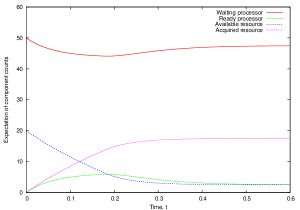
(a) ODE approximation: mean

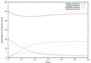
(b) Simulation: mean

Figure 1: Comparison of the simulation averages and numerical solution to the corresponding approximating ODEs for the processor/resource model.

It can be useful to know not just the average counts of states at each time but also the variability of these counts. For the stochastic simulation, this can be achieved by calculating the variance instead of just the mean. For the ODE approximation, it has been shown in [1] how to adapt the existing techniques to produce systems of ODEs approximating higher moments of state counts. Figure 2 compares a numerical solution to these ODEs with the variance obtained from the stochastic simulation.

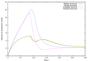
(a) ODE approximation: variance

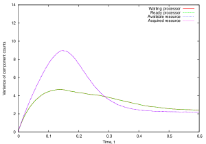
(b) Simulation: variance

Figure 2: Comparison of the variance for the processor/resource model obtained from the stochastic simulation with their ODE approximation.

It is apparent that the ODE approximation is not equally accurate for the whole observed time. Figure 1 and even more so Figure 2 shows that the error of the approximation starts just before the time $t=0.2$.

The main focus of our work is to investigate, with the help of an efficient software tool, why this error appears and to provide practical means of detecting it without running the computationally expensive simulation. We will explain, using results from [1], that it occurs due to models passing through so-called switch points, when the total rate of cooperating actions between groups of components becomes equal.

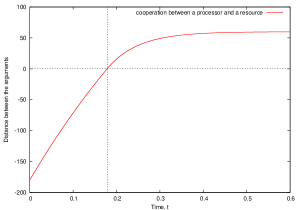
Figure 3: Switch point plot showing the difference between total rate of processors and resources component groups. The switch point occurs when the plot goes through zero.

We present a tool that will visualise the distance that an evolving model is from a switch point. Figure 3 shows this for the processor and resource model and confirms that the error in the variance approximation coincides with the switch point in total rate between processors and resources just before $t=0.2$.

In this work, we will consider models described in an extension of the stochastic process algebra PEPA. Section 1.3 provides a brief introduction to Grouped PEPA. In Section 1.3.1 we will overview the method of deriving ODE approximations to higher moments of PEPA models.

It was shown in [10] that the error of this approximation for the mean decreases as we increase the initial populations (e.g. $m$ and $n$ in this example). Section 1.5 gives a theoretical justification that a similar convergence can be expected to hold in the case of the variance ODE approximation.

It is important to note that although we are studying switch points in the context of PEPA models, switch points also occur in other performance modelling settings. Specifically, they occur whenever there is a contention for a finite pool of resources which may be saturated by demand. The most obvious example of this is an $M/M/n$ queue which has $n$ servers, and a service rate of $\mu$ at each server; the total service rate when $k$ jobs are in the system is given by $\min(n\mu,k\mu)$, where $k=n$ defines the switch point of this queue.

Section 2 introduces a tool that for the first time implements higher order moment approximation for a stochastic process algebra. This tool is used for our investigations in Section 3, where we present cases studies of different switch point behaviour and also demonstrate instances of the results from Section 1.5.

1.2 Related Tools

There are many tools that support analysis of very large state spaces in performance modelling. Two such popular tools which have good support for explicit state-space analysis are Möbius and PRISM.

The Möbius [11] framework has perhaps the widest user base with implementations of many formalisms, including stochastic process algebras (SPAs), stochastic automata networks (SANs) and generalised stochastic Petri nets (GSPNs). Möbius supports a distributed simulation environment and numerical solvers for models of up to tens of millions of states.

PRISM [6] is a probabilistic model checker which supports low level formalisms such as DTMCs, CTMCs and Markov Decision Processes (MDPs) with an analysis engine based on Binary Decision Diagrams (BDDs) and Multi-Terminal Binary Decision Diagrams (MTBDDs). PRISM can analyse models of up to $10^{11}$ states, however this can depend heavily on the model being studied and on detailed considerations such as the exact variable ordering in the underlying MTBDD.

Performance tools that support differential-equation based analysis have been primarily designed around stochastic process algebras such as stochastic $\pi$-calculus and PEPA. For $\pi$-calculus SPiM [12, 13] has long been the standard tool for simulating stochastic $\pi$ calculus models, but being a simulator it suffers from scalability issues for models with very large populations of components. A recent tool, JSPiM [14], allows for the chemical ground form subset of stochastic $\pi$-calculus to be analysed via differential equations. For the stochastic process algebra PEPA, the tools ipc [15, 16] and the Eclipse PEPA plug-in [17] implement the so-called fluid translation [3] to produce sets of differential equations for PEPA.

In the field of biological modelling, tools such as Dizzy [18] and SPiM have been used to capture first order approximations to system dynamics using a combination of stochastic simulation [19] and differential equation approximation. A recent tool from [20] generates ODEs approximating higher moments of models using the mass-action kinetics and described in the Systems Biology mark-up language. However for the reasons discussed, these techniques do not extend to computer and communication system modelling.

The tool presented here provides a framework implementation for a variant of PEPA known as Grouped PEPA or GPEPA [21]. Using the established relationship between the underlying discrete Markov process and the fluid model [1], we can for the first time produce higher moments through differential equation analysis of massive models. The relationship with the underlying discrete model also allows us to identify areas of possible inaccuracy where the fluid model is known to be least accurate. Finally the GPEPA analyser (GPA) allows comparison by stochastic simulation, where this is feasible.

1.3 Grouped PEPA models

Grouped PEPA or GPEPA [1] is a simple syntactic extension of PEPA. A brief summary of PEPA is given in Appendix A. GPEPA is defined to provide a more elegant treatment of the ODE moment approximation (and also allowing a more elegant implementation). Formally, the extension introduces a further level in the syntax of PEPA, the Grouped PEPA models, defined as:

$$M::=M\raisebox{-4.30554pt}{$\;\stackrel{{\scriptstyle\mbox{\large$\rhd\lhd$}}}{{\scriptscriptstyle L}}\,$}M~{}\mid{\mathbf{Y}}\{P\parallel\cdots\parallel P\}$$

This defines a GPEPA model to be either a PEPA cooperation between two GPEPA models (over the set of actions $L$) or alternatively a labelled grouping of PEPA components, $P$, in parallel with each other. ${\mathbf{Y}}$ is the group label. The Grouped PEPA model is nothing more than the standard PEPA model with, additionally, a label to define the components involved in parallel grouping. These labels will be later used to define the level at which the ODE approximation to the system is made.

The example from Section 1.1 can be represented by the following GPEPA definition:

$${\mathit{Processor}}_{0} \stackrel{{\scriptstyle\mbox{\em{\tiny def}}}}{{=}}({\mathit{acquire}},\,r_{1}).{\mathit{Processor}}_{1} {\mathit{Resource}}_{0} \stackrel{{\scriptstyle\mbox{\em{\tiny def}}}}{{=}}({\mathit{acquire}},\,r_{2}).{\mathit{Resource}}_{1}$$

$${\mathit{Processor}}_{1} \stackrel{{\scriptstyle\mbox{\em{\tiny def}}}}{{=}}({\mathit{task}},\,q).{\mathit{Processor}}_{0} {\mathit{Resource}}_{1} \stackrel{{\scriptstyle\mbox{\em{\tiny def}}}}{{=}}({\mathit{reset}},\,s).{\mathit{Resource}}_{0}$$

$${\mathit{System}}\stackrel{{\scriptstyle\mbox{\em{\tiny def}}}}{{=}}{\mathbf{Processors}}\{{\mathit{Processor}}_{0}[m]\}\raisebox{-4.30554pt}{$\;\stackrel{{\scriptstyle\mbox{\large$\rhd\lhd$}}}{{\scriptscriptstyle\{{\mathit{acquire}}\}}}\,$}{\mathbf{Resources}}\{{\mathit{Resource}}_{0}[n]\}$$

The choice of labels (${\mathbf{Processors}}$ and ${\mathbf{Resources}}$) was arbitrary and will serve to identify each state of the system by counting the occurrences of ${\mathit{Processor}}_{0}$ and ${\mathit{Processor}}_{1}$ processes in the group ${\mathbf{Processors}}$ and occurrences of ${\mathit{Resource}}_{0}$ and ${\mathit{Resource}}_{1}$ in the group ${\mathbf{Resources}}$.

1.3.1 ODE analysis

The states in PEPA models originally keep track of the state of each individual sequential component. This can lead to state space explosion, which makes the model not amenable to traditional analysis methods other than the computationally expensive stochastic simulation. The state space explosion is especially severe (with respect to the syntactical size of the model) in the case of models with groups consisting of many components acting in parallel. An established way to tackle this in the case of groups consisting of many identical components is by aggregating the state space by keeping track of counts of the individual components [3]. In the context of Grouped PEPA models, it is sufficient to represent each state of the underlying CTMC by a numerical vector $\mathbf{N}(t)$ consisting of counts $N_{G,P}(t)$ for each possible pair of group label $G$ and component $P$ (as in [1]).

Allowing this to be a real-valued vector $\mathbf{v}(t)$ (with components accordingly named $v_{G,P}(t)$), a system of ordinary differential equations, $\dot{\mathbf{v}}(t)=\mathbf{f}(\mathbf{v}(t))$ with initial conditions $\mathbf{v}(0)=\mathbf{N}(0)$ can be intuitively derived from the corresponding PEPA description. These ODEs deterministically approximate the PEPA model’s evolution over time. This has been formally shown in [1] (by comparison with the Chapman–Kolmogorov equations for the underlying CTMC) to be an approximation to the expectation of the individual group/component counts, i.e. $\mathbf{v}(t)\approx\mathbb{E}[\mathbf{N}(t)]$.

The authors of [1] further extended this method to derive ODE approximations to higher and joint moments of the counts, such as variances, covariances and others. The number of differential equations generated by this method, when calculating all the moments of order up to $p$, is proportional to $n^{p}$ where $n$ is the number of component derivatives.

The method generalises the vectors $\mathbf{N}$ and $\mathbf{v}$ to include components for values (integers and reals respectively) of each possible moment of the group/component pair counting processes. For example $\mathbf{N}(t)$ can include the squared count of component $P$ within a group $G$, $N_{(P,G)}^{2}(t)$ and $\mathbf{v}(t)$ an approximation to its expectation, i.e. $v_{(P,G)^{2}}(t)\approx\mathbb{E}[N_{(P,G)}^{2}(t)]$.

A general advantage of this approximation to the moments (including the mean) is that the resulting system of ODEs can be numerically integrated by standard methods. This usually requires less computation than running sufficiently many replications of the respective stochastic simulation over the same model.

1.3.2 Two-stage Client/Server Example

We will look at a more complicated example that will be used in the following investigations. Consider a client/server model, where communication occurs in two stages. Clients first request a server to communicate with. After admitting a request from a server, a client moves to a waiting state and the corresponding server to a ready state. Then, any ready server can serve a waiting client, after which the client can perform a required task and the server returns to the idle state. Additionally, an idle server can break, requiring a reset. This can be represented by the following PEPA components:

$${\mathit{Client}} \stackrel{{\scriptstyle\mbox{\em{\tiny def}}}}{{=}} ({\mathit{request}},{r\!}_{{\mathit{req}}}).{\mathit{Client}}\_{\mathit{waiting}}$$

$${\mathit{Client}}\_{\mathit{waiting}} \stackrel{{\scriptstyle\mbox{\em{\tiny def}}}}{{=}} ({\mathit{data}},{r\!}_{{\mathit{data}}}).{\mathit{Client}}\_{\mathit{think}}$$

$${\mathit{Client}}\_{\mathit{think}} \stackrel{{\scriptstyle\mbox{\em{\tiny def}}}}{{=}} ({\mathit{think}},{r\!}_{{\mathit{think}}}).{\mathit{Client}}$$

$${\mathit{Server}} \stackrel{{\scriptstyle\mbox{\em{\tiny def}}}}{{=}} ({\mathit{request}},{r\!}_{{\mathit{req}}}).{\mathit{Server}}\_{\mathit{get}}+({\mathit{break}},{r\!}_{{\mathit{break}}}).{\mathit{Server}}\_{\mathit{broken}}$$

$${\mathit{Server}}\_{\mathit{get}} \stackrel{{\scriptstyle\mbox{\em{\tiny def}}}}{{=}} ({\mathit{data}},{r\!}_{{\mathit{data}}}).{\mathit{Server}}$$

$${\mathit{Server}}\_{\mathit{broken}} \stackrel{{\scriptstyle\mbox{\em{\tiny def}}}}{{=}} ({\mathit{reset}},{r\!}_{{\mathit{{\mathit{reset}}}}}).{\mathit{Server}}$$

composed into the GPEPA system equation defined by $CS(c,s)$ over the set of actions $L=\{{\mathit{request}},{\mathit{data}}\}$:

$$CS(c,s)={\mathbf{Clients}}\{{\mathit{Client}}[c]\}\raisebox{-4.30554pt}{$\;\stackrel{{\scriptstyle\mbox{\large$\rhd\lhd$}}}{{\scriptscriptstyle L}}\,$}{\mathbf{Servers}}\{{\mathit{Server}}[s]\}$$

The aggregation described above represents each derivative state of the model at each time $t$ as a vector $\mathbf{N}(t)$, i.e. the underlying CTMC can be treated as a vector valued stochastic process, with components $N_{{\mathbf{Clients}},P}(t)$, where $P$ can be ${\mathit{Client}}$, ${\mathit{Client}}\_{\mathit{waiting}}$ or ${\mathit{Client}}\_{\mathit{think}}$ and $N_{{\mathbf{Servers}},Q}(t)$ where $Q$ can be ${\mathit{Server}}$, ${\mathit{Server}}\_{\mathit{get}}$ or ${\mathit{Server}}\_{\mathit{broken}}$. The ODE approximation generates a system of ODEs, $\dot{\mathbf{v}}(t)=\mathbf{f}(\mathbf{v}(t))$ with a real-valued vector solution $\mathbf{v}(t)$ with the same components as the vector $\mathbf{N}(t)$ and initial conditions $v_{{\mathbf{Clients}},{\mathit{Client}}}(0)=N_{{\mathbf{Clients}},{\mathit{Client}}}(0)=c$, $v_{{\mathbf{Servers}},{\mathit{Server}}}(0)=N_{{\mathbf{Servers}},{\mathit{Server}}}(0)=s$ and $v_{G,P}(0)=0$ otherwise. See Section 1.5 for the exact formulation of $\mathbf{f}(\mathbf{v}(t))$.

1.4 Nature of the approximations

The nature of the approximation of the system of ODEs to the CTMC evolution boils down to the approximation of the rate at which two components evolve in cooperation (as discussed originally in [1]).

This is trivial in the unsurprising case of purely concurrent models, where no cooperation takes part. For these, the approximation is exact and can directly replace moment calculation via stochastic simulation.

In general, the rate of cooperation can be of the form $\mathbf{r}(\mathbf{N}(t))\cdot\min(\mathbf{f}(\mathbf{N}(t)),\mathbf{g}(\mathbf{N}(t)))$ where $\mathbf{r}(\cdot)$ is a rational function of piecewise linear functions and $\mathbf{f}(\cdot)$ and $\mathbf{g}(\cdot)$ are piecewise linear functions all of the components of $\mathbf{N}(t)$. The functions $\mathbf{f}(\mathbf{N}(t))$ and $\mathbf{g}(\mathbf{N}(t))$ are a calculation of the total rates of cooperating actions being enabled in cooperating component groups.

For a certain class of models called the split-free models, introduced in [1], it can be shown that the function $\mathbf{r}$ is constant and $\mathbf{f},\mathbf{g}$ are piecewise linear. It then turns out that the nature of the deterministic approximation of $\mathbf{N}(t)$ by $\mathbf{v}(t)$ depends on the approximation

$$\mathbb{E}[\min(\mathbf{f}(\mathbf{N}(t)),\mathbf{g}(\mathbf{N}(t))]\approx\min(\mathbf{f}(\mathbb{E}[\mathbf{N}(t)]),\mathbf{g}(\mathbb{E}[\mathbf{N}(t)]))$$ (1.1)

where the right hand side is approximated by $\min(\mathbf{f}(\mathbf{v}(t)),\mathbf{g}(\mathbf{v}(t)))$. Note that the functions $\mathbf{f}$ and $\mathbf{g}$ may also include further minimum terms themselves and thus induce multiple further applications of the approximation not shown explicitly above. It is argued in [1] that the error of this approximation is at its highest around so-called switch points. These occur when the total rate of cooperating action between component groups becomes equal and hence $\mathbf{f}(\mathbf{N}(t))=\mathbf{g}(\mathbf{N}(t))$ causing the $\min$ function to switch.

One of the main contributions of this paper is to verify and further investigate this claim empirically. We will be able to use our GPEPA tool to identify the switch points and to display the error in the ODE approximation around the switch points of a given GPEPA model. We will focus on first order switch points: those coming from a $\min$ term involving no higher orders than means of component counts.

The switch points are also defined for general GPEPA models. However, for those, the nature of the ODE moment approximation also depends on the approximation of terms, $\mathbb{E}[\mathbf{r}(\mathbf{N}(t))]$ for a rational function $\mathbf{r}(\cdot)$. Our GPEPA tool allows analysis of these models, by using the approximation $\mathbf{r}(\mathbb{E}[\mathbf{N}(t)])$. However, in our first investigation we concentrate on the split-free models. We will be using the client/server model $CS(c,s)$ from the above section, as it can be easily shown to be split-free.

1.5 Theoretical considerations

In this section, we aim to provide justification for the convergence of the suitably-scaled mean and variance ODE approximations as the component population sizes are increased.

In order to do this, we will more formally set up some notation to allow us to consider general GPEPA models and their associated systems of ODEs in a compact manner. For a general GPEPA model, assume that we have a vector-valued stochastic process $\mathbf{N}(t)$, defined on $\mathbb{R}_{+}$ taking values in $\mathbb{Z}_{+}^{N}\subset\mathbb{R}_{+}^{N}$, for some $N\in\mathbb{Z}_{+}$. In line with Section 1.3.1, each component of this process counts the number of a particular derivative state currently active in a parallel group of the model, of which there are $N$ derivative states in total, across all parallel groups.

Analogously, we define the vector-valued deterministic function $\mathbf{v}(t)$, also defined on $\mathbb{R}_{+}$ and taking values in $\mathbb{R}_{+}^{N}$ to be the ODE approximation to the expectation of this model. We assume that it is defined uniquely by the system of differential equations $\dot{\mathbf{v}}(t)=\mathbf{f}(\mathbf{v}(t))$ and the initial condition $\mathbf{v}(0)=\mathbf{N}(0)$. As discussed above, the exact form of the deterministic function $\mathbf{f}:\mathbb{R}_{+}^{N}\rightarrow\mathbb{R}^{N}$ is given in [1] and corresponds component-wise to the rate at which each derivative state is incremented, minus that at which it is decremented, in a given state of the model. It helps now to consider the system of ODEs explicitly for an example model. Indeed, in the case of the client/server example of Section 1.3.2, we have a total of six derivative states, giving $N=6$,

$$\begin{split}\mathbf{N}(t)&\equiv(N_{C}(t),\,N_{C_{w}}(t),\,N_{C_{t}}(t),\,N_{S}(t),\,N_{S_{g}}(t),\,N_{S_{b}}(t))^{\text{T}}\\ \mathbf{v}(t)&\equiv(v_{C}(t),\,v_{C_{w}}(t),\,v_{C_{t}}(t),\,v_{S}(t),\,v_{S_{g}}(t),\,v_{S_{b}}(t))^{\text{T}}\end{split}$$

and:

$$\mathbf{f}(\mathbf{v}(t))\equiv\begin{pmatrix}-\min(v_{S}(t),\,v_{C}(t)){r\!}_{{\mathit{req}}}+v_{C_{t}}(t){r\!}_{{\mathit{think}}}\\ -\min(v_{C_{w}}(t),\,v_{S_{g}}(t)){r\!}_{{\mathit{data}}}+\min(v_{S}(t),\,v_{C}(t)){r\!}_{{\mathit{req}}}\\ -v_{C_{t}}(t){r\!}_{{\mathit{think}}}+\min(v_{C_{w}}(t),\,v_{S_{g}}(t)){r\!}_{{\mathit{data}}}\\ -\min(v_{S}(t),\,v_{C}(t)){r\!}_{{\mathit{req}}}-v_{S}(t){r\!}_{{\mathit{break}}}+\min(v_{C_{w}}(t),\,v_{S_{g}}(t)){r\!}_{{\mathit{data}}}+v_{S_{b}}(t){r\!}_{{\mathit{{\mathit{reset}}}}}\\ -\min(v_{C_{w}}(t),\,v_{S_{g}}(t)){r\!}_{{\mathit{data}}}+\min(v_{S}(t),\,v_{C}(t)){r\!}_{{\mathit{req}}}\\ -v_{S_{b}}(t){r\!}_{{\mathit{{\mathit{reset}}}}}+v_{S}(t){r\!}_{{\mathit{break}}}\end{pmatrix}$$

where we have used an appropriate shorthand notation for the components of $\mathbf{N}(t)$ and $\mathbf{v}(t)$. In order to make the desired theoretical considerations in this section, it is necessary to consider a structurally equivalent sequence of GPEPA models which have the same structure of parallel component groups and differ only in terms of the size of the component populations within these groups. Furthermore, we require that they all have the same initial proportion of each component type in each case. For such a sequence of GPEPA models, let $\{\mathbf{N}^{i}(t)\}_{i=1}^{\mathchar 561\relax}$ be their associated stochastic counting processes in the notation above, and for each $i$, write $S_{i}:=N^{i}_{1}(t)+\cdots+N^{i}_{n}(t)$ for the total component population of model $i$. So our requirement of constant initial component type proportions is stated formally as:

$$\frac{N^{i}_{k}(0)}{S_{i}}=\frac{N^{j}_{k}(0)}{S_{j}}\text{ for all $i,\,j>0$ and $k\in\{1,\,\ldots,\,n\}$}$$

In the case of (G)PEPA, it is relatively straightforward to see that for any $\mathbf{x}\in\mathbb{R}_{+}^{N}$, $\mathbf{f}(k\mathbf{x})=k\mathbf{f}(\mathbf{x})$ for all $k\in\mathbb{R}_{+}$. Furthermore, since the GPEPA models in our sequence differ only in terms of their initial component counts, it is easy to see that the function $\mathbf{f}(\cdot)$ is the same for any $i$. These two facts together mean that we need only define the fluid approximation to $\mathbf{N}^{i}(t)$, say, $\mathbf{v}^{i}(t)$ for a particular value of $i$, and the fluid approximation for any other $i$ can be defined in terms of it. Indeed, for any $i,\,j>0$, if $\dot{\mathbf{v}}^{i}(t)=\mathbf{f}(\mathbf{v}^{i}(t))$ and $\dot{\mathbf{v}}^{j}(t)=\mathbf{f}(\mathbf{v}^{j}(t))$ with initial conditions, $\mathbf{v}^{i}(0)=\mathbf{N}^{i}(0)$ and $\mathbf{v}^{j}(0)=\mathbf{N}^{j}(0)$, respectively, we have:

$$\mathbf{v}^{i}(0)=\mathbf{v}^{j}(0)\times\frac{S_{i}}{S_{j}}\text{ and }\mathbf{v}^{i}(t)=\mathbf{v}^{j}(t)\times\frac{S_{i}}{S_{j}}\text{ for all $t>0$ }$$

Thus for the rest of this section, we consider the quantity $\mathbf{\bar{v}}(t):=\mathbf{v}^{i}(t)/S_{i}$, for all $t>0$, which we have just seen is independent of $i$.

1.5.1 Convergence of mean approximation

It is shown in [10], based on a result by Kurtz [22], that, in the above notation for any sequence of structurally equivalent GPEPA models, the following holds:

Theorem 1.1

If $S_{i}\rightarrow\mathchar 561\relax$ as $i\rightarrow\mathchar 561\relax$ then:

$$\frac{1}{S_{i}}\mathbb{E}[\mathbf{N}^{i}(t)]\rightarrow\mathbf{\bar{v}}(t)$$

as $i\rightarrow\mathchar 561\relax$, uniformly over bounded intervals $t\in[0,\,T)$.

This demonstrates that, in the limit of component population size, the mean number of components at time $t$ does indeed tend towards the ODE solution. An example of this convergence is shown in Figure 6(a), Section 3.

1.5.2 Convergence of variance approximation

In this section, we provide theoretical support for our hypothesis that in the limit of large populations and under an appropriate scaling, the variance of component counts converges to the approximation given by the ODEs for split-free GPEPA models.

We will start by approximating the GPEPA model’s underlying CTMC, $\mathbf{N}^{i}(t)$, as the sum of a deterministic process, $\mathbf{\bar{v}}(t)$, given by the first order ODEs, and a Gaussian process, $\mathbf{E}(t)$ defined below. From this description, we will derive a set of ODEs describing the evolution of the covariances of the Gaussian process. These can be formally shown (Theorem 1.2) to agree with the covariances of the CTMC in the limit of a sequence of GPEPA models of increasing size. We will argue that the second moment ODEs from the CTMC (Section 1.3.1) capture the dynamics of the system more accurately than the ODEs generated from the Gaussian process. This provides the basis for our hypothesis that the variances of the CTMC do indeed converge to the solution to the second moment ODEs from Section 1.3.1 as the population size increases.

The decomposition described above gives the following approximation to the underlying CTMC of a GPEPA model:

$$\mathbf{N}^{i}(t)\approx S_{i}\mathbf{\bar{v}}(t)+\sqrt{S_{i}}\mathbf{E}(t)$$ (1.2)

where $\mathbf{E}(t)$ is the Gaussian process mentioned above. In order to proceed with defining $\mathbf{E}(t)$, it is necessary to enumerate explicitly the transitions in the aggregated state space of the GPEPA model. Assume that there are $K$ such transitions and, following [23], let $\{\mathbf{l}^{k}\in\mathbb{Z}^{N}\}_{k=1}^{K}$ be the sequence of jump vectors, specifying that if the $k$th such transition occurs at time $t$, $\mathbf{N}(t)=\mathbf{N}(t-)+\mathbf{l}^{k}$, where $t-$ is the instant immediately preceding $t$. Then define rate functions, $\{f^{k}:\mathbb{R}_{+}^{N}\rightarrow\mathbb{R}_{+}\}_{k=1}^{K}$, specifying the aggregate rate of each transition. In the case of the client/server example, we have $K=5$ (for the $5$ possible activities) and:

$$\begin{array}[]{lll}\mathbf{l}^{1}=(-1,\,1,\,0,\,-1,\,1,\,0)&&f^{1}(\mathbf{x})=\min(x_{1},\,x_{4})\,{r\!}_{{\mathit{req}}}\\ \mathbf{l}^{2}=(0,\,-1,\,1,\,1,\,-1,\,0)&&f^{2}(\mathbf{x})=\min(x_{2},\,x_{5})\,{r\!}_{{\mathit{data}}}\\ \mathbf{l}^{3}=(1,\,0,\,-1,\,0,\,0,\,0)&&f^{3}(\mathbf{x})=x_{3}\,{r\!}_{{\mathit{think}}}\\ \mathbf{l}^{4}=(0,\,0,\,0,\,-1,\,0,\,1)&&f^{4}(\mathbf{x})=x_{4}\,{r\!}_{{\mathit{break}}}\\ \mathbf{l}^{5}=(0,\,0,\,0,\,1,\,0,\,-1)&&f^{5}(\mathbf{x})=x_{6}\,{r\!}_{{\mathit{{\mathit{reset}}}}}\end{array}$$

The stochastic process $\mathbf{E}(t)$ is now given in the following theorem [23], which applies to any sequence of structurally equivalent split-free GPEPA models with underlying CTMCs $\{\mathbf{N}_{i}(t)\}_{i=1}^{\mathchar 561\relax}$, corresponding model sizes $\{S_{i}\}_{i=1}^{\mathchar 561\relax}$ and rescaled ODE approximation $\mathbf{\bar{v}}(t)$.

Theorem 1.2 below defines the Gaussian process $\mathbf{E}(t)$ in terms of time-scaled Wiener processes, $W^{k}(t)$. Readers unfamiliar with Wiener processes and weak convergence of stochastic processes can consult for instance Rogers and Williams [24] or Klebaner [25]. The set $\hat{\mathbf{T}}$ defined in the theorem can be given more intuitively as the set of all times at which two arguments of a minimum function in the right-hand side, $\mathbf{f}(\mathbf{\bar{v}}(t))$, of the first moment ODEs are equal.

Theorem 1.2

Let $T>0$ and let $\hat{\mathbf{T}}$ be the subset of $\{t\in[0,\,T)\}$ for which $\mathbf{f}(\cdot)$ is not totally differentiable at the point $\mathbf{\bar{v}}(t)$. We require that $\hat{\mathbf{T}}$ has Lebesgue measure zero. Then on all of $[0,\,T)\setminus\hat{\mathbf{T}}$, $\mathbf{f}(\cdot)$ has a well-defined Jacobian at the point $\mathbf{\bar{v}}(t)$, say $D\,\mathbf{f}(\mathbf{\bar{v}}(t))$. Extend this to all points $\{\mathbf{\bar{v}}(t)\,:\,t\in[0,\,T)\}$, say by defining it to be the matrix of zeros at times in $\hat{\mathbf{T}}$.

Then if $S_{i}\rightarrow\mathchar 561\relax$ as $i\rightarrow\mathchar 561\relax$, $\frac{\mathbf{N}^{i}(t)}{\sqrt{S_{i}}}-\sqrt{S_{i}}\mathbf{\bar{v}}(t)\Rightarrow\mathbf{E}(t)$ also as $i\rightarrow\mathchar 561\relax$, where:

$$\mathbf{E}(t):=\int_{0}^{t}D\,\mathbf{f}(\mathbf{\bar{v}}(s))\cdot\mathbf{E}(s)\,{\rm d}s+\sum_{k\in K}W^{k}\left(\int_{0}^{t}f^{k}(\mathbf{\bar{v}}(s))\,{\rm d}s\right)\mathbf{l}^{k}$$

and $\{W^{k}(t)\}_{k=1}^{K}$ is a sequence of $K$ mutually independent standard Wiener processes (aka Brownian motions). The convergence ($\Rightarrow$) is weak convergence in $D_{\mathbb{R}_{+}^{N}}[0,\,T)$, the space of $\mathbb{R}_{+}^{N}$-valued càdlàg functions.

This is essentially a generalisation of a result of Kurtz [26] to cope with the case of non-smooth rate functions as introduced in the case of PEPA models, or other formalisms for modelling synchronisation in computer systems, by the minimum functions. It can be shown that the process $\mathbf{E}(t)$ is the unique solution of the following (Itō) stochastic differential equation (SDE):

$${\rm d}\mathbf{E}(t)=\mathbf{\mu}(\mathbf{E}(t),\,t)\,{\rm d}t+\mathbf{\sigma}(t)\,{\rm d}\mathbf{W}(t)$$

where $\mathbf{\mu}(\mathbf{x},\,t):\mathbb{R}^{N}\times\mathbb{R}_{+}\rightarrow\mathbb{R}^{N}$ and $\mathbf{\sigma}(t):\mathbb{R}_{+}\rightarrow\mathbb{R}^{N\times K}$ are defined by:

$$\mathbf{\mu}(\mathbf{x},\,t):=D\,\mathbf{f}(\mathbf{\bar{v}}(t))\cdot\mathbf{x},\qquad\mathbf{\sigma}(t):=\left(l^{j}_{i}\times\sqrt{f^{j}(\mathbf{\bar{v}}(t))}\right)_{ij}$$

and $\mathbf{W}(t):=(W^{1}(t),\,\ldots,\,W^{K}(t))^{\text{T}}$ is a $K$-dimensional standard Wiener process. This representation allows us to apply the machinery of Itō’s Lemma, see for example [24, 27], to derive the following system of ODEs, whose unique solution is exactly the covariance matrix of $\mathbf{E}(t)$:

$$\frac{\rm d}{{\rm d}t}\mathbf{Cov}[\mathbf{E}(t),\,\mathbf{E}(t)]={} \mathbf{Cov}[\mathbf{E}(t),\,\mathbf{E}(t)]\,(D\,\mathbf{f}(\mathbf{\bar{v}}(t)))^{\text{T}}+D\,\mathbf{f}(\mathbf{\bar{v}}(t))\,\mathbf{Cov}[\mathbf{E}(t),\,\mathbf{E}(t)]^{\text{T}}+\sum_{k\in K}f^{k}(\mathbf{\bar{v}}(t))\,\mathbf{l}^{k}\,(\mathbf{l}^{k})^{\text{T}}$$ (1.3)

If we apply this to the client/server example for the specific covariance $E_{S}(t)$, corresponding to the ${\mathit{Server}}$ component of $\mathbf{N}(t)$, $N_{S}(t)$, we have:

$$\frac{\rm d}{{\rm d}t}\text{Cov}[E_{S}(t),\,E_{S}(t)]={} -2\,{r\!}_{{\mathit{req}}}\left(\mathbf{1}_{\{\bar{v}_{S}(t)\leq\bar{v}_{C}(t)\}}\text{Cov}[E_{S}(t),\,E_{S}(t)]+\mathbf{1}_{\{\bar{v}_{S}(t)>\bar{v}_{C}(t)\}}\text{Cov}[E_{S}(t),\,E_{C}(t)]\right)$$

$$+2\,{r\!}_{{\mathit{data}}}\left(\mathbf{1}_{\{\bar{v}_{S_{g}}(t)\leq\bar{v}_{C_{w}}(t)\}}\text{Cov}[E_{S}(t),\,E_{S_{g}}(t)]+\mathbf{1}_{\{\bar{v}_{S_{g}}(t)>\bar{v}_{C_{w}}(t)\}}\text{Cov}[E_{S}(t),\,E_{C_{w}}(t)]\right)$$

$$-2\,{r\!}_{{\mathit{break}}}\text{Cov}[E_{S}(t),\,E_{S}(t)]+2\,{r\!}_{{\mathit{{\mathit{reset}}}}}\text{Cov}[E_{S}(t),\,E_{S_{b}}(t)]$$

$$+{r\!}_{{\mathit{req}}}\min(\bar{v}_{C}(t),\,\bar{v}_{S}(t))+{r\!}_{{\mathit{data}}}\min(\bar{v}_{C_{w}}(t),\,\bar{v}_{S_{g}}(t))+{r\!}_{{\mathit{break}}}\bar{v}_{S}(t)+{r\!}_{{\mathit{{\mathit{reset}}}}}\bar{v}_{S_{b}}(t)$$ (1.4)

Note that Theorem 1.2 suggests the approximation:

$$\mathbf{Cov}[N_{S}(t),\,N_{S}(t)]\approx\mathbf{Cov}[S\bar{v}_{S}(t)+\sqrt{S}E_{S}(t),\,S\bar{v}_{S}(t)+\sqrt{S}E_{S}(t)]=S\,\mathbf{Cov}[E_{S}(t),\,E_{S}(t)]$$

where $S$ is taken as the total population of clients and servers. Indeed, in general, Theorem 1.2 implies (assuming its hypothesis), as $i\rightarrow\mathchar 561\relax$, if $S_{i}\rightarrow\mathchar 561\relax$, that:

$$\frac{1}{S_{i}}\,\mathbf{Cov}[\mathbf{N}^{i}(t),\,\mathbf{N}^{i}(t)]\rightarrow\mathbf{Cov}[\mathbf{E}(t),\,\mathbf{E}(t)]$$

So the system of ODEs given in Equation (1.3) yields an approximation to the covariance matrix of the underlying CTMC of a general GPEPA model. Furthermore, as we have just seen, this approximation is guaranteed by Theorem 1.2 to converge in the limit of large populations.

However, the covariance ODE approximation implemented by the GPA tool consists of integrating a slightly different system of ODEs. Our intention now is to show that they are very similar to those of Equation (1.3) and in fact can intuitively be regarded as a better approximation to the actual covariance matrix of the CTMC. This is the basis of our conjecture that a similar convergence result also holds, and furthermore, that the rate of convergence may well be faster for the ODEs implemented in the GPA tool.

In more detail for our example, applying the techniques of [1] for the specific term $\text{Cov}[N_{S}(t),\,N_{S}(t)]$, we obtain the exact differential equation:

$$\frac{\rm d}{{\rm d}t}\text{Cov}[N_{S}(t),\,N_{S}(t)]={} \frac{\rm d}{{\rm d}t}\mathbb{E}[N_{S}^{2}(t)]-2\mathbb{E}[N_{S}(t)]\frac{\rm d}{{\rm d}t}\mathbb{E}[N_{S}(t)]$$

$$={} -2\,{r\!}_{{\mathit{req}}}\biggl{(}\mathbb{E}[\min(N_{C}(t)\,N_{S}(t),\,N_{S}^{2}(t))]-\mathbb{E}[\min(N_{C}(t),\,N_{S}(t))]\mathbb{E}[N_{S}(t)]\biggl{)}$$

$$+2\,{r\!}_{{\mathit{data}}}\biggl{(}\mathbb{E}[\min(N_{C_{w}}(t)\,N_{S}(t),\,N_{S_{g}}\,N_{S}(t))]-\mathbb{E}[\min(N_{C_{w}}(t),\,N_{S_{g}}(t))]\mathbb{E}[N_{S}(t)]\biggl{)}$$

$$-2\,{r\!}_{{\mathit{break}}}\biggl{(}\mathbb{E}[N_{S}^{2}(t)]-\mathbb{E}^{2}[N_{S}(t)]\biggl{)}$$

$$+2\,{r\!}_{{\mathit{{\mathit{reset}}}}}\biggl{(}\mathbb{E}[N_{S_{b}}(t)\,N_{S}(t)]-\mathbb{E}[N_{S_{b}}(t)]\,\mathbb{E}[N_{S}(t)]\biggl{)}$$

$$+{r\!}_{{\mathit{req}}}\,\mathbb{E}[\min(N_{C}(t),\,N_{S}(t))]+{r\!}_{{\mathit{data}}}\,\mathbb{E}[\min(N_{C_{w}}(t),\,N_{S_{g}}(t))]$$

$$+{r\!}_{{\mathit{break}}}\,\mathbb{E}[N_{S}(t)]+{r\!}_{{\mathit{{\mathit{reset}}}}}\,\mathbb{E}[N_{S_{b}}(t)]$$ (1.5)

Since the corresponding system of ODEs cannot be solved analytically or numerically due to the presence of expectations of non-linear functions, the approximation $\mathbb{E}[\min(X,\,Y)]\approx\min(\mathbb{E}[X],\,\mathbb{E}[Y])$ can be applied repeatedly as in [1] and Section 1.4 to deduce approximate ODEs for $\text{Cov}[N_{S}(t),\,N_{S}(t)]$ and the other covariances. This system of ODEs can then be solved numerically as implemented in general by the GPA tool.

There are two kinds of approximations being applied here, those which we might call first-order, such as $\mathbb{E}[\min(N_{C}(t),\,N_{S}(t))]\approx\min(\mathbb{E}[N_{C}(t)],\,\mathbb{E}[N_{S}(t)])$, and those which we might call second-order, such as $\mathbb{E}[\min(N_{C}(t)\,N_{S}(t),\,N_{S}^{2}(t))]\approx\min(\mathbb{E}[N_{C}(t)\,N_{S}(t)],\,\mathbb{E}[N_{S}^{2}(t)])$. The key point to note now is that if we keep the first-order approximations the same but replace the second-order approximations by ones of the form:

$$\mathbb{E}[\min(N_{C}(t)\,N_{S}(t),\,N_{S}^{2}(t))]\approx\mathbf{1}_{\{\mathbb{E}[N_{S}(t)]>\mathbb{E}[N_{C}(t)]\}}\,\mathbb{E}[N_{C}(t)\,N_{S}(t))]+\mathbf{1}_{\{\mathbb{E}[N_{S}(t)]\leq\mathbb{E}[N_{C}(t)]\}}\,\mathbb{E}[N_{S}^{2}(t)]$$

then we recover the system of ODEs of Equation (1.3). This is a reasonable approximation, but we switch second-order minimum terms by making only first-order comparisons. It is thus intuitively clear that it is likely to be a worse approximation than the second moment ODEs derived from the CTMC.

On this basis, we might reasonably expect that the covariance ODE approximations, derived from the CTMC and implemented by the GPA tool, should converge to the actual covariances when scaled by the total component population size. An example of this can be seen in Figure 6(b), Section 3.

2 GPA: The GPEPA Analyser

In this section we introduce a new tool for analysing Grouped PEPA models. The Grouped PEPA analyser (GPA) uses the results from [1], briefly described above, as a basis for producing deterministic approximations of transient behaviour of syntactically specified Grouped PEPA models. It can also use these to provide passage-time approximations from [10].

GPA in addition implements stochastic simulation of the models to allow investigations into the nature of the approximation and the convergence results from Section 1.5. In the next section, we look at some specific examples that empirically demonstrate this. We first give an overview of GPA, giving its syntax and the commands it provides.

2.1 Overview

The syntax of models specified in GPA is very close to the formal language of Grouped PEPA. Each GPA model starts with definitions of parameters used as rates in component definitions and parameters used as initial counts in the grouped model definitions. The definitions of individual PEPA components then follow. Finally, a single Grouped PEPA model is given, using the defined components.

Groups are specified by labels with components enclosed in braces { }. Multiple components of the same type are given by [n] written after the component identifier, where n is a previously-defined parameter. The cooperation operator is represented by the cooperation set enclosed in angled brackets < >.

The GPEPA model corresponding to the example from Section 1.1 can be represented in GPA as:

 r1=2.0; q=14.0;  m=50.0;                r2=14.0; s=2.0;  n=20.0;Processor0 = (acquire,r1).Processor1;   Resource0 = (acquire,r2).Resource1;Processor1 = (task,q).Processor0;       Resource1 = (reset,s).Resource0;      Processors{Processor0[m]}<acquire>Resources{Resource0[n]} 

Appendix C contains the grammar describing the full syntax of GPA.

2.2 ODE Analysis and Comparison with Simulation

On each GPA model, several analyses can be performed. Each analysis is specified with required parameters (for example, the time range we are interested in for the transient behaviour of the model), after the analysis name. Following this is a list of commands that allow visualisation and further manipulation of the resulting data points.

The ODE analysis provides analysis of the given model by a deterministic approximation via a set of ordinary differential equations as described in Section 1.3.1. The enclosed commands determine the maximum order that has to be considered in calculations. For example, if the commands involve only plots of means and variances of component counts, differential equations for approximation of all the possible (joint) moments of order $1$ and $2$ are implicitly generated. These ODEs are then numerically integrated (using a fourth-order Runge–Kutta solver). The parameter stopTime specifies the time over which the numerical solution is given. Parameter stepSize determines the fixed time interval between each successive pair of data points that are taken. The parameter density specifies the accuracy by telling the solver how many sub-intervals should each time interval between the data points be divided into. The following GPA code performs an ODE analysis on the above GPA model, displaying: mean counts of ${\mathit{Processor}}_{0}$ components in group ${\mathbf{Processors}}$ and ${\mathit{Resource}}_{0}$ components in group ${\mathbf{Resources}}$ and model switch points:

 odes(stopTime = 3.0,stepSize = 0.001,density=10){     plot(E[Processors:Processor0],E[Resources:Resource0]);     plotSwitchpoints(1); ...} 

The Simulation analysis provides analysis of models by stochastic simulation of their underlying continuous time Markov chain. GPA generates a representation of the CTMC and uses the Gillespie algorithm [19] to simulate the CTMC at given time intervals until the simulation stop time is reached.

The stochastic simulation is repeated several times (given by the parameter replications) and then averaged to provide the final data set. On the above model, the following code performs a simulation analysis to extract the same mean component counts as before:

 simulation(stopTime = 3.0,stepSize = 0.001,replications=1000){     plot(E[Processors:Processor0],E[Resources:Resource0]); ...} 

To compare results from stochastic simulation and ODE analysis, the Comparison analysis provides a way of calculating the difference between the two analyses. It takes a simulation and ODE analysis as parameters (which are required to have the same stop time and step size) and calculates the difference between their resulting data points. All the enclosed commands then use this difference in the same way as data points for the other analyses. For example, a comparison of the above analyses:

 comparison(    odes(stopTime=3.0,stepSize=0.001,density=1000){...},    simulation(stopTime=3.0,stepSize=0.001,replications=1000){...}){        plot(E[Processors:Processor0],E[Resources:Resource0]);} 

2.3 Commands and Functionality

GPA can plot results from these analyses itself or output raw data by means of an optional file redirection.

The plot command provides direct plots of different arithmetic expressions involving (higher order and joint) moments of component counts and numerical constants. Each group–component pair is identified by the syntax group:component. A moment is an expectation, with syntax E[], of products of these, for example E[G1:C1^2 G2:C2]. Several shorthands are provided, such as the variance represented by Var[G:C] (which stands for E[G:C^2]-E[G:C]^2), and Cov[G1:C1,G2:C2] which represents the covariance of two component count variables and the $n$th central moment represented by Central[G:C,n]. The following commands are examples of the above:

 plot(Var[Processors:Processor1],Var[Resources:Resource1]);plot(Central[Processors:Processor1,4]);plot(E[Resources:Resource0]+E[Resources:Resource1]); The plotSwitchpoints command inside an ODE analysis visualises distance from switch points in the ODE approximation. It obtains a set of all the occurrences of the $\min$ function (containing only moments of order upto a given integer argument) in the moment ODEs. For each data point from the ODE analysis, the command plots the difference between the two arguments of each of the $\min$ occurrences. The switch points then correspond to the zero points of this plot.

One of the reasons the plot command provides arithmetic expressions of the moments is to give GPA the flexibility to obtain approximations of passage times. As described in [10], the passage time approximations and the corresponding bounds can be expressed as certain functions of the (higher order) moments. We will explore this functionality in a later paper, but suffice to say that the accuracy of the passage-time approximations depends critically on the ODE approximation of first and higher moments.

Some example plots showing error comparisons in variances for the processor/resource model can be found in Appendix B. For further details on GPA, including random model generation for testing purposes, we refer the interested reader to the freely available source code obtainable from [28].

3 Numerical Investigation: Two-stage Client/Server

In this section, we investigate empirically the nature of the ODE approximations as mentioned in Section 1.4 and the convergence results from Section 1.5. More specifically, we will check that the simulation variances converge to the ODE approximations as the initial component populations scale up. We also look at higher moments to suggest a possible result analogous to the one mentioned in Section 1.5.2. We will look at the error of the ODE approximation of the moments and quantitative properties of the convergence, in the context of the switch points defined in Section 1.4.

In order to investigate this, we use two models - one which does not stay near a switch point in any large time interval (we will informally refer to it as to the occasionally switching model) and one which steadily stays near a switch point for a longer period of time (we will informally refer to it as to the persistently switching model).

In both cases we will use the two-stage client/server model from Section 1.3.2, with two sets of parameters and taking the client population, $c=100$, and the server population, $s=50$:

$$\text{Model A}: \qquad r_{\mathit{req}}=2.0 \qquad r_{\mathit{break}}=0.1 \qquad r_{\mathit{think}}=0.20 \qquad r_{\mathit{data}}=1.0 \qquad r_{\mathit{reset}}=2.0$$

$$\text{Model B}: \qquad r_{\mathit{req}}=2.0 \qquad r_{\mathit{break}}=0.3 \qquad r_{\mathit{think}}=0.35 \qquad r_{\mathit{data}}=2.0 \qquad r_{\mathit{reset}}=0.05$$

The switch point behaviour for these examples can be seen on Figure 4. There are two possible sources of switch points in the client/server model, each corresponding to an instance of cooperation in the model. One, the term $\min(v_{\mathit{Client}}(t)\cdot r_{\mathit{req}},v_{\mathit{Server}}(t)\cdot r_{\mathit{req}})$, comes from the cooperation when a client establishes connection with a server. Another, $\min(v_{{\mathit{Client}}_{\mathit{waiting}}}(t)\cdot r_{\mathit{data}},v_{{\mathit{Server}}_{\mathit{get}}}(t)\cdot t_{\mathit{data}})$, comes from the cooperation when a client retrieves data from an available server.

For the $\min$ term involving ${\mathit{Server}}_{\mathit{get}}$ and ${\mathit{Client}}_{\mathit{waiting}}$, the model hits infinitely many switch points. These do not influence the error of the approximation since the two corresponding counting processes are stochastically identical, so there is no error in the corresponding expectation approximation. For the $\min$ term involving the ${\mathit{Client}}$ and ${\mathit{Server}}$ components, in the first, simpler case, the model hits one switch point at time $t\simeq 2.1$, but does not stay around any switch point for a period of time. The second model hits two switch points when $t\simeq 2.8$ and $t\simeq 4.8$ and stays close to a switch point in the time interval between them.

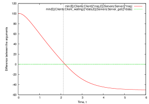
(a) Switch point plot for Model A

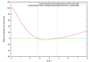
(b) Switch point plot for Model B

Figure 4: First order switch points for the two-stage client/server models

In the following sections, we will look at the errors in moment approximation for both of the above models and compare them in the context of these switch points. We will look at the expectation, variance, skewness and kurtosis (the standardised third and fourth central moments) of the component counts for each model and its respective versions with initial populations scaled by a factor of $n=1,4,16$ and $64$. We investigate how the scale influences the error of the ODE approximation. For each scale, we plot the difference between the moments from simulation and their approximation, specially near the times where a switch point is encountered. It is worth noting that these times are the same across all $n$, since the ODEs for the means are scale invariant, as was mentioned in Section 1.5.

In line with the considerations from Section 1.5, we normalise the error of expectation and variance approximations dividing by the total component population. We plot the errors of the skewness and kurtosis approximations (standardised third and fourth central moments, respectively) without any additional normalisation.

3.1 Model A: Occasionally switching model

First, we look at the simpler case, Model A, in which the client/server model does not stay near a switch point for a longer period of time. We start by comparing side by side, for the first three central moments, the simulation average with its ODE approximation in Figure 5.

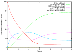
(a) ODE approximation: mean

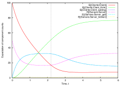
(b) Simulation: mean

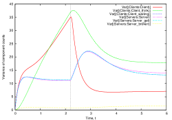
(c) ODE approximation: variance

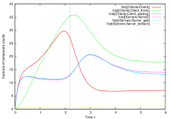
(d) Simulation: variance

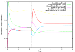
(e) ODE approximation: skewness

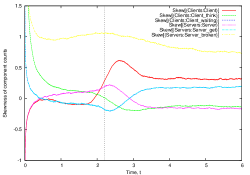
(f) Simulation: skewness

Figure 5: Moments from simulation and approximation for the two-stage client/server model, Model A.

For kurtosis (not shown), similar to the skewness, the approximation is quite accurate when the model is not near a switch point, but errors are visible otherwise.

For all four moments the ODE approximation is qualitatively close to the simulation average. However, there are visible quantitative differences starting at the variance and getting worse with the skewness and kurtosis. This is especially noticeable for the moments involving the number of ${\mathit{Client}}$ components and in the time interval around the first order switch point from Figure 4 (shown by the vertical line on the plots in Figure 5). We plot the actual error of the approximation (using the GPA comparison analysis) for these moments, for each of the scaled versions of the model, in Figure 6.

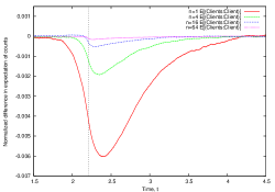
(a) Normalised error: mean

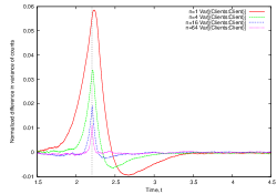
(b) Normalised error: variance

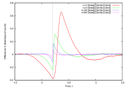
(c) Absolute error: skewness

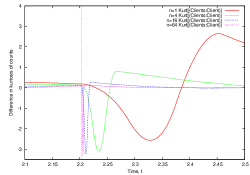
(d) Absolute error: kurtosis

Figure 6: The influence of scaling of Model A on the normalised error around the switch point events

3.2 Model B: Persistently switching model

Figure 7 shows the mean and variance for the case where the model stays near a switch point for a longer interval of time in Model B. The mean seems quite accurate, but the error in variance approximation is high around the interval where the model stays near a switch point.

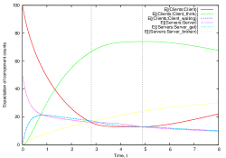
(a) ODE approximation: mean

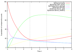
(b) Simulation: mean

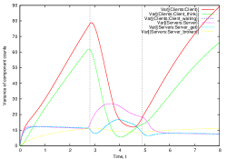
(c) ODE approximation: variance

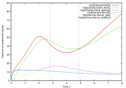
(d) Simulation: variance

Figure 7: Moments from simulation and approximation for the two-stage client/server model, Model B. The ODE approximation is quite accurate for the mean, but large differences are visible for the variance.

Figure 8 looks at the error more closely and plots the difference between the moments from simulation and their ODE approximation for the ${\mathit{Client}}$ component, for different scales of Model B. It can be seen that the normalised error in Figure 8 is much higher than in the case of Model A. We believe this is caused by the fact that the model is closer to the switch points. However, in both cases we can confirm that the error for the mean and variance seems to be going to zero in the scale limit, but concentrated most around a switch point. The same seems to be the case for the skewness. For kurtosis, it seems that the error does not necessarily get smaller in value, but the interval where it appears seems to get smaller with increased scale.

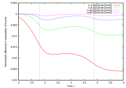
(a) Normalised error: mean

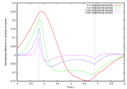
(b) Normalised error: variance

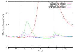
(c) Absolute error: skewness

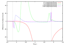
(d) Absolute error: kurtosis

Figure 8: The influence of scaling of Model B on the normalised error around the switch point events

Section 1.5 shows that the marginal distributions of component counts become normal as the populations are increased. The normal distribution has a constant skewness and kurtosis (0 and 3 respectively). We can check the plots for the simulations to verify this. This seems to be the case for the ODE approximation, except perhaps for the points concentrated around the switch point times.

4 Conclusion and future work

We introduced a tool, GPA [28], that for the first time makes available the ODE approximations of higher moments to a wide range of models described in an extension of the PEPA stochastic process algebra. We used the tool to carry out investigations into the nature of the ODE approximation, that will help the modellers to detect errors without running computationally more expensive stochastic simulations. We theoretically justified that the variance of the component counts converges to the ODE approximation as the initial populations are scaled and with the help of our tool verified this for a simple example.

We observed, for a model where the resulting differential equations are piecewise linear, that the error is influenced by how closely the model stays near the switch points during its time evolution. If the model only crosses switch points at certain points of time and does not stay near any during the rest of the time, then the error is concentrated tightly around those switch point events. We also saw that, with increasing scale of initial component populations, the error in the ODE solution becomes even more tightly concentrated around the switch point. If the model stays near switch points for longer periods of time, the resulting error is much more severe and decreases more slowly with increased scale of the initial populations.

These observations help us to assess the validity of the ODE approximation without actually running the simulations. For a given model, we can use GPA to visualise the switch point behaviour of the model and use the intuition gained from our investigations to say whether the approximation is accurate.

Moreover, the presented results and observations are not just specific to the PEPA stochastic process algebra. The $\min$ functions with the concept of switch points appear in situations when there is a competition for multiple resources, for example multi-server queues or many-server semantics stochastic Petri nets. Therefore we believe that the gained insight is relevant to a wider area within performance modelling of computer systems.

In future, we plan to develop methods that would be able to quantify the error (e.g. in terms of bounds obtained from the distance from a switch point), thus making GPA able to warn the modeller of the potential magnitude of any error. We also plan to investigate the sensitivity of the switch point behaviour to changes in the rates and initial population parameters to allow deliberate generation of accurate ODE approximation.

Appendix A PEPA Summary

We briefly introduce PEPA [29], a simple stochastic process algebra with sufficient expressiveness to model a wide variety of systems. As in various other process algebras, systems in PEPA are represented as compositions of components which undertake actions thus evolving into further components. Each action has a rate, interpreted as a parameter of an exponential random variable that governs the delay associated with the action. This means that the stochastic behaviour of the model can be described as a CTMC.

The basic building blocks of PEPA are sequential components, described by the syntax

$$S::=(\alpha,r).S~{}\mid~{}S+S~{}\mid~{}C_{S}$$

where $C_{S}$ stands for a constant that defines a sequential component. Intuitively, the component $(\alpha,r).S$ can undertake the action $\alpha$ with rate $r$ and evolve into the component $S$. The component $P+Q$ has a choice to undertake actions that both $P$ and $Q$ can undertake.

The sequential components can be composed in parallel to form model components, described by the syntax

$$P::=P\raisebox{-4.30554pt}{$\;\stackrel{{\scriptstyle\mbox{\large$\rhd\lhd$}}}{{\scriptscriptstyle L}}\,$}P~{}\mid~{}P/L~{}\mid~{}C$$

where $C$ is a constant defining any PEPA component. The component $P\raisebox{-4.30554pt}{$\;\stackrel{{\scriptstyle\mbox{\large$\rhd\lhd$}}}{{\scriptscriptstyle L}}\,$}Q$ enables cooperation between $P$ and $Q$ by only allowing $P$ and $Q$ to evolve together when undertaking an action from the cooperation set $L$. The cooperation influences the rate of the common evolution. PEPA assumes bounded capacity: a component cannot be made to perform an activity faster by cooperation, so the resulting rate is the minimum of the cooperating rates. This is discussed in more detail in [29]. For actions not in $L$, $P$ and $Q$ can evolve independently with no influence on the rates. If $L$ is the empty set, we use the shorthand $P\parallel Q$ meaning that $P$ and $Q$ are purely concurrent and don’t synchronise. We also use the shorthand $P[n]$ for $n$ purely concurrent copies of $P$.

The syntax $P/L$ stands for action hiding. For simplicity, we will not consider this feature in the presented work, however, it should be straightforward to include using the results from [1].

The full details of the operational semantics of PEPA can be found in [29].

Appendix B Processor/Resource Variance Plots

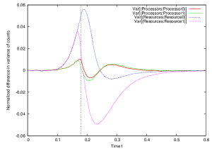
(a) Normalised difference in variance

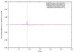
(b) Normalised difference in variance for the scaled version

Figure 9: Difference in variance between the simulation and its ODE approximation for the processor/resource model, produced by the comparison analysis.

Figures 1, 2 and 3 that we used in the initial example in Section 1.1 were all produced by the respective GPA commands enclosed in simulation and ODE analyses. We could examine the error of the approximation more closely by using the comparison analyses. Figure 9 compares the error in variance approximation for the processors resource model with $m=50$ and $n=20$ with a version with populations scaled by $100$, i.e. with $m=5000$ and $2000$. In order to demonstrate the results from Section 1.5, the difference is scaled by the population size $m+n$. We can see that under this scaling, the relative error does decrease.

Appendix C GPA syntax definition

Models

$$\mathit{System} :=\mathit{ParameterDefinition}^{\ast}~{}\mathit{ComponentDefinition}^{\ast}~{}\mathit{ModelDefinition}~{}\mathit{Analysis}^{\ast}$$

$$\mathit{ParameterDefinition} :=\mathit{parameterId}~{}{\color[rgb]{0,0,1}\mathtt{=}}~{}\mathit{realnumber}{\color[rgb]{0,0,1}\mathtt{;}}$$

$$\mathit{ComponentDefinition} :=\mathit{componentID}~{}{\color[rgb]{0,0,1}\mathtt{=}}~{}\mathit{Component}$$

$$\mathit{Component} :=\mathit{Component}{\color[rgb]{0,0,1}\mathtt{<}}\mathit{ActionList}^{?}{\color[rgb]{0,0,1}\mathtt{>}}\mathit{Component}$$

$$\phantom{:=}~{}\mid\mathit{Summation}\mid\mathit{componentId}\mid{\color[rgb]{0,0,1}\mathtt{(}}\mathit{Component}{\color[rgb]{0,0,1}\mathtt{)}}$$

$$\mathit{Summation} :=\mathit{Prefix}({\color[rgb]{0,0,1}\mathtt{+}}\mathit{Prefix})^{\ast}$$

$$\mathit{Prefix} :={\color[rgb]{0,0,1}\mathtt{(}}\mathit{actionId}{\color[rgb]{0,0,1}\mathtt{,}}~{}\mathit{parameterId}~{}{\color[rgb]{0,0,1}\mathtt{).}}({\color[rgb]{0,0,1}\mathtt{(}}\mathit{Summation}{\color[rgb]{0,0,1}\mathtt{)}}\mid{\color[rgb]{0,0,1}\mathtt{stop}}\mid\mathit{componentId}\mid){\color[rgb]{0,0,1}\mathtt{;}}$$

$$\mathit{ModelDefinition} :={\color[rgb]{0,0,1}\mathtt{(}}\mathit{ModelDefinition}{\color[rgb]{0,0,1}\mathtt{<}}\mathit{ActionList}^{?}{\color[rgb]{0,0,1}\mathtt{>}}\mathit{ModelDefinition}{\color[rgb]{0,0,1}\mathtt{)}}$$

$$\phantom{:=}~{}\mid\mathit{groupLabel}{\color[rgb]{0,0,1}\mathtt{\{}}\mathit{ComponentsParallel}{\color[rgb]{0,0,1}\mathtt{\}}}$$

$$\mathit{ComponentsParallel} :=\mathit{Component}(~{}{\color[rgb]{0,0,1}\mathtt{|}}\mathit{Component})^{\ast}$$

$$\mathit{Component} :=\mathit{componentId}~{}({\color[rgb]{0,0,1}\mathtt{[}}\mathit{parameterId}{\color[rgb]{0,0,1}\mathtt{]}})^{?}$$

$$\mathit{ActionList} :=\mathit{actionId}~{}({\color[rgb]{0,0,1}\mathtt{,}}~{}\mathit{actionId})^{\ast}$$

Analyses

$$\mathit{Analysis} :=\mathit{ODEs}~{}|~{}\mathit{Simulation}\mid\mathit{Comparison}$$

$$\mathit{ODEs} :={\color[rgb]{0,0,1}\mathtt{odes(stopTime=}}\mathit{realnumber}{\color[rgb]{0,0,1}\mathtt{,stepSize=}}\mathit{realnumber}{\color[rgb]{0,0,1}\mathtt{,density=}}\mathit{integer}{\color[rgb]{0,0,1}\mathtt{)}}$$

$$\phantom{:=}~{}~{}~{}{\color[rgb]{0,0,1}\mathtt{\{}}\mathit{Command}^{\ast}{\color[rgb]{0,0,1}\mathtt{\}}}$$

$$\mathit{Simulation} :={\color[rgb]{0,0,1}\mathtt{simulation(stopTime=}}\mathit{realnumber}{\color[rgb]{0,0,1}\mathtt{,stepSize=}}\mathit{realnumber}{\color[rgb]{0,0,1}\mathtt{,replications=}}\mathit{integer}{\color[rgb]{0,0,1}\mathtt{)}}$$

$$\phantom{:=}~{}~{}~{}{\color[rgb]{0,0,1}\mathtt{\{}}\mathit{Command}^{\ast}{\color[rgb]{0,0,1}\mathtt{\}}}$$

$$\mathit{Comparison} :={\color[rgb]{0,0,1}\mathtt{comparsion(}}\mathit{ODEs}{\color[rgb]{0,0,1}\mathtt{,}}\mathit{Simulation}{\color[rgb]{0,0,1}\mathtt{)\{}}\mathit{Command}^{\ast}{\color[rgb]{0,0,1}\mathtt{\}}}$$

Commands

$$\mathit{Command} :=\mathit{CommandNoFile}({\color[rgb]{0,0,1}\mathtt{\texttt{->}"}}\mathit{filename}{\color[rgb]{0,0,1}\mathtt{"}})^{?}{\color[rgb]{0,0,1}\mathtt{;}}$$

$$\mathit{CommandNoFile} :={\color[rgb]{0,0,1}\mathtt{plot(}}\mathit{MomentExpressions}{\color[rgb]{0,0,1}\mathtt{)}}\mid{\color[rgb]{0,0,1}\mathtt{plotSwitchpoints(}}\mathit{integer}{\color[rgb]{0,0,1}\mathtt{)}}$$

$$\mathit{MomentExpressions} :=\mathit{MomentExpression}({\color[rgb]{0,0,1}\mathtt{,}}~{}\mathit{MomentExpression})^{\ast}$$

$$\mathit{MomentExpression} :=\mathit{MomentExpression}({\color[rgb]{0,0,1}\mathtt{+}}\mid{\color[rgb]{0,0,1}\mathtt{-}}\mid{\color[rgb]{0,0,1}\mathtt{*}}\mid{\color[rgb]{0,0,1}\mathtt{/}}\mid{\color[rgb]{0,0,1}\mathtt{\textrm{\^{}}}})\mathit{MomentExpression}$$

$$\phantom{:=}~{}\mid{\color[rgb]{0,0,1}\mathtt{E[}}\mathit{Moment}({\color[rgb]{0,0,1}\mathtt{+}}\mathit{Moment})^{\ast}{\color[rgb]{0,0,1}\mathtt{]}}\mid{\color[rgb]{0,0,1}\mathtt{Var[}}\mathit{GCPair}({\color[rgb]{0,0,1}\mathtt{+}}\mathit{GCPair})^{\ast}{\color[rgb]{0,0,1}\mathtt{]}}$$

$$\phantom{:=}~{}\mid({\color[rgb]{0,0,1}\mathtt{Standardised}})^{?}{\color[rgb]{0,0,1}\mathtt{Central[}}\mathit{GCPair}{\color[rgb]{0,0,1}\mathtt{,}}\mathit{integer}{\color[rgb]{0,0,1}\mathtt{]}}$$

$$\phantom{:=}~{}\mid\mathit{realnumber}\mid\mathit{parameterId}\mid{\color[rgb]{0,0,1}\mathtt{(}}\mathit{MomentExpression}{\color[rgb]{0,0,1}\mathtt{)}}$$

$$\mathit{Moment} :=(\mathit{GCPair}({\color[rgb]{0,0,1}\mathtt{\textrm{\^{}}}}\mathit{integer})^{?})^{+}$$

$$\mathit{GCPair} :=\mathit{groupLabel}{\color[rgb]{0,0,1}\mathtt{:}}\mathit{Component}$$

References

- [1] R. Hayden and J. T. Bradley, “A fluid analysis framework for a Markovian process algebra,” Theoretical Computer Science, vol. 411, pp. 2260–2297, May 2010. doi://10.1016/j.tcs.2010.02.001.
- [2] L. Bortolussi and A. Policriti, “Stochastic concurrent constraint programming and differential equations,” in QAPL’07, 5th Workshop on Quantitative Aspects of Programming Languages, vol. 190 of Electronic Notes in Theoretical Computer Science, pp. 27–42, September 2007.
- [3] J. Hillston, “Fluid flow approximation of PEPA models,” in QEST’05, Proceedings of the 2nd International Conference on Quantitative Evaluation of Systems, (Torino), pp. 33–42, IEEE Computer Society Press, September 2005.
- [4] L. Cardelli, “On process rate semantics,” Theoretical Computer Science, vol. 391, pp. 190–215, February 2008.
- [5] W. J. Knottenbelt, P. G. Harrison, M. S. Mestern, and P. S. Kritzinger, “A probabilistic dynamic technique for the distributed generation of very large state spaces,” Performance Evaluation, vol. 39, pp. 127–148, February 2000.
- [6] M. Kwiatkowska, G. Norman, and D. Parker, “PRISM: Probabilistic symbolic model checker,” in TOOLS’02, Proceedings of the 12th International Conference on Modelling Techniques and Tools for Computer Performance Evaluation (A. J. Field et al., ed.), vol. 2324 of Lecture Notes in Computer Science, (London), pp. 200–204, Springer-Verlag, 2002.
- [7] D. T. Gillespie, Markov Processes: An Introduction for Physical Scientists. Academic Press, 1991.
- [8] N. G. van Kampen, Stohastic Processes in Physics and Chemistry. North Holland, 2007.
- [9] C. H. Lee, K.-H. Kim, and P. Kim, “A moment closure method for stochastic reaction networks,” Journal of Chemical Physics, vol. 130, pp. 1–15, April 2009.
- [10] R. Hayden and J. T. Bradley, “Fluid passage-time calculation in large Markov models,” Performance Evaluation, 2008. (submitted).
- [11] D. D. Deavours, G. Clark, T. Courtney, D. Daly, S. Derisavi, J. M. Doyle, W. H. Sanders, and P. G. Webster, “The Möbius framework and its implementation,” IEEE Transactions on Software Engineering, vol. 28, pp. 956–969, October 2002.
- [12] A. Phillips and L. Cardelli, “A correct abstract machine for the stochastic pi-calculus,” in BIOCONCUR’04, Concurrent Models in Molecular Biology, August 2004. Workshop proceedings.
- [13] A. Phillips and L. Cardelli, “Efficient, correct simulation of biological processes in stochastic Pi-calculus,” in CMSB’07, Proceedings of Computational Methods in Systems Biology, vol. 4695 of Lecture Notes in Computer Science, pp. 184––199, Springer-Verlag, September 2007.
- [14] A. Stefanek, “Continuous and spatial extension of stochastic pi-calculus,” Master’s thesis, Department of Computing, Imperial College London, July 2009.
- [15] A. Clark, “The ipclib PEPA library,” in QEST’07, 4th International Conference on the Quantitative Evaluation of Systems, pp. 55–56, IEEE, September 2007.
- [16] J. T. Bradley, N. J. Dingle, S. T. Gilmore, and W. J. Knottenbelt, “Derivation of passage-time densities in PEPA models using ipc: the Imperial PEPA Compiler,” in MASCOTS’03, Proceedings of the 11th IEEE/ACM International Symposium on Modeling, Analysis and Simulation of Computer and Telecommunications Systems, pp. 344–351, IEEE, October 2003.
- [17] M. Tribastone, “The PEPA plug-in project,” in QEST’07, Proceedings of the 4th Int. Conference on the Quantitative Evaluation of Systems, pp. 53–54, IEEE Computer Society, September 2007.
- [18] S. Ramsey, D. Orrell, and H. Bolouri, “Dizzy: Stochastic simulation of large-scale genetic regulatory networks,” Journal of Bioinformatics and Computational Biology, vol. 3, no. 2, pp. 415–436, 2005.
- [19] D. T. Gillespie, “Exact stochastic simulation of coupled chemical reactions,” Journal of Physical Chemistry, vol. 81, no. 25, pp. 2340–2361, 1977.
- [20] C. S. Gillespie, “Moment-closure approximations for mass-action models,” IET Systems Biology, vol. 3, no. 1, pp. 52–58, 2009.
- [21] R. Hayden and J. T. Bradley, “Evaluating fluid semantics for passive stochastic process algebra cooperation,” Performance Evaluation, 2010. (In press).
- [22] T. Kurtz, “Solutions of ordinary differential equations as limits of pure jump Markov processes,” vol. 7, pp. 49–58, April 1970.
- [23] R. Hayden and J. T. Bradley, “A functional central limit theorem for PEPA,” in PASTA’09, Proceedings of the 8th Workshop on Process Algebra and Stochastically Timed Activities, (Edinburgh), pp. 13–23, August 2009.
- [24] L. C. G. Rogers and D. Williams, Diffusions, Markov Processes and Martingales, vol. 1. Cambridge University Press, 2nd ed., 2000.
- [25] F. C. Klebaner, Introduction to Stochastic Calculus with Applications. Imperial College Press, 2nd ed., 2005.
- [26] T. Kurtz, “Strong approximation theorems for density dependent Markov chains,” Stochastic Processes and Applications, vol. 6, pp. 223–240, 1978.
- [27] O. Kallenberg, Foundations of Modern Probability. Springer, 2002.
- [28] “Grouped PEPA analyzer.” http://doc.ic.ac.uk/~as1005/GPA.
- [29] J. Hillston, A Compositional Approach to Performance Modelling, vol. 12 of Distinguished Dissertations in Computer Science. Cambridge University Press, 1996.