A Two-dimensional Model of Shear-flow Transition

Abstract

We explore a two-dimensional dynamical system modeling transition in shear flows to try to understand the nature of an ’edge’ state. The latter is an invariant set in phase space separating the basin of attraction $B$ of the laminar state into two parts distinguished from one another by the nature of relaminarizing orbits. The model is parametrized by $R$, a stand-in for Reynolds number. The origin is a stable equilibrium point for all values of $R$ and represents the laminar flow. The system possesses four critical parameter values at which qualitative changes take place, $R_{sn},R_{h},R_{bh}$ and $R_{\infty}$. The origin is globally stable if $R<R_{sn}$ but for $R>R_{sn}$ has two further equilibrium points, $X_{lb}$ and $X_{ub}$. Of these $X_{lb}$ is unstable for all values of $R>R_{sn}$ whereas $X_{ub}$ is stable for $R<R_{bh}$ and therefore possesses its own basin of attraction $D$. At $R=R_{h}$ a homoclinic bifurcation takes place with the simultaneous formation of a homoclinic loop and an edge state.

For $R_{h}<R<R_{bh}$ the edge state, which is the stable manifold of $X_{lb}$, forms part of $\partial B$, the boundary of the basin of attraction of the origin. The other part of $\partial B$ is a periodic orbit $P$ bounding $D$. $P$ and $D$ shrink with increasing $R$. At $R=R_{bh}$ there is a ’backwards Hopf’ bifurcation at which $X_{ub}$ loses its stability and $P$ and $D$ disappear. For $R_{bh}<R<R_{\infty}$ the edge is ’pure’ in the sense that it is the only phase space structure that lies outside the basin of attraction of the origin. As $R$ increases the point $X_{lb}$ recedes to progressively greater distances, with a singularity at $R=R_{\infty}$ where it becomes infinite. For $R>R_{\infty}$ $X_{lb}$ has reappeared, the edge state has disappeared, and the geometrical structure favors permanent transition from the laminar state, increasingly so for increasing values of $R$.

1 Introduction

Transition to turbulence in shear flows occurs as the relevant parameter, the Reynolds number $R$, increases beyond a critical value. This transition differs in important respects from the onset of instability in other familiar problems of hydrodynamics and indeed of other familiar problems in applied mathematics. One difference of long standing is that the transition takes place while the unperturbed, laminar flow remains asymptotically stable ([5],[6]). A related difference is that the transition is not sharp: the value of the critical Reynolds number for onset depends on the size and nature of the perturbation.

Another difference is that the transition may not be permanent. For a range of $R$ values, an apparently complex motion occurs for a while but is then followed by relaminarization. This regime of a return to the laminar state after a complex motion has been found in numerical calculations and related to the occurrence of an ’edge’ state ([5],[1]). Sometimes the complex motion has a chaotic character and one refers to the ’edge of chaos.’ These features have been found both in the behavior of low-dimensional models of shear flows and in numerical treatments of the Navier-Stokes equations. In these theoretical treatments the edge seems to be a codimension-one surface in phase space separating relaminarizing orbits of two different types: orbits of one type relaminarize quickly, whereas those of other type relaminarize more slowly and follow a more complicated trajectory than orbits of the first type (cf [9]). An alternative picture in which the edge is a pair of surfaces very close together was proposed in [7] but seems implausible in light of the conclusions of the present paper (see §5 below).

The object of the present note is to exhibit a two-dimensional model in which some of the features described above – particularly the edge state – emerge in a transparent manner. The choice of model is in some respects arbitrary, and the fact that it is two-dimensional excludes a variety of behaviors that are possible in the Navier-Stokes equations. It may nevertheless be useful in supplying an internally consistent template for the behavior of such systems. In our model the laminar state is represented by the origin of coordinates and ’relaminarization’ of an orbit means that it tends to the origin as $t\to+\infty$. Before we turn to this model (§3), a word about the basin of attraction.

2 The basin of attraction

The basin of attraction $B$ of an asymptotically stable equilibrium point $q$ is the set of initial-data points whose orbits tend to $q$ as $t\to+\infty$. By the boundary of $B$, $\partial B$, we mean here the set of points $p$ whose every neighborhood contains both points that are in $B$ and points that are not in $B$. There are simple examples for which $\partial B$ separates phase space into two regions, $B$ and a complementary region $D$ in which no orbit tends to $q$. It is worthwhile emphasizing that the definition of $\partial B$ does not require this simple picture to hold.

One simple example is

$$\dot{x}=-x(1-x^{2}-y^{2})-y,\;\dot{y}=x-y(1-x^{2}-y^{2}),$$ (1)

which becomes $\dot{r}=-r(1-r^{2}),\;\dot{\theta}=1$ in polar coordinates. There is a stable equilibrium point at the origin ($q=0$). Orbits for which $r(0)<1$ relaminarize and the basin of attraction is precisely the set $r<1$. Orbits for which $r(0)\geq 1$ never relaminarize.

The ’edge’ picture of Eckhardt et al (cf [9]) is more complex. It seems to imply a near-global stability of the laminar point in the sense that virtually all orbits relaminarize. There must be exceptions – invariant sets like equilibrium points or periodic orbits – and the edge itself appears to be an invariant set. But these exceptions are of lower dimension then the ambient space so, with probability one, all orbits relaminarize. This picture, which is arrived at through numerical computations, could of course be a consequence of incomplete numerical sampling: there could be undiscovered, open, invariant sets somewhere in phase space.

The simple system (1) above, which has no edge state, is not designed to model shear flows. We now examine a two-dimensional system that is designed to model shear flows, and does have an edge state.

3 Systems of shear-flow type

Finite-dimensional systems that mimic shear flows possess the following characteristics: they have only linear and quadratic terms, the linear terms feature a non-normal matrix and the nonlinear terms conserve energy (cf [7]). We consider the following family of two-dimensional systems of this kind:

$$\dot{x}_{1}=-\delta x_{1}+x_{2}+b_{1}x_{1}x_{2}-b_{2}x_{2}^{2},$$ (2)

$$\dot{x}_{2}=-\delta x_{2}-b_{1}x_{1}^{2}+b_{2}x_{1}x_{2}.$$ (3)

The shear-flow problem is characterized by a Reynolds number $R$ and this appears in these equations through the relation $\delta=1/R$. The real parameters $b_{1},b_{2}$ could be chosen arbitrarily, but in the numerical examples below we have chosen $b_{1}=1,b_{2}=3$. The laminar flow is represented by the equilibrium solution $(x_{1},x_{2})=(0,0)=O$.

Further equilibrium solutions of the system (2) can be expressed as follows:

$$x_{1}=\frac{C\delta}{Cb_{2}-b_{1}}\mbox{ and }x_{2}=Cx_{1}$$ (4)

where

$$C=\left(1\pm\sqrt{1-4\delta^{2}}\right)/2\delta=\left(R\pm\sqrt{R^{2}-4}\right)/2$$ (5)

Equation (5) shows that two real equilibrium points other than the origin $O$ occur if and only if $R>2$. This identifies the ’saddle-node’ critical value as $R_{sn}=2$ in the present case. It is not difficult to show that the origin is asymptotically stable if $R<2$. For $R>2$ we’ll denote by $X_{lb}$ the equilibrium point obtained when the minus sign is chosen in equation (5) and by $X_{ub}$ the point obtained when the plus sign is chosen. For the choices $b_{1}=1$ and $b_{2}=3$ we get Figure 1, showing the norm of an equilibrium solution plotted against $R$.

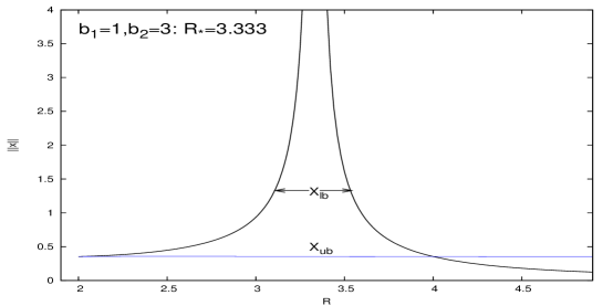
Figure 1: The abscissa $\|x\|=0$ represents the stable, laminar point. The apparent cusp at the saddle-node point $R=2$ is an artifact of the special choice $b_{1}=1$ and $b_{2}=3$ and applies only to the norm: the individual components $x_{1}$ and $x_{2}$ have a smooth (parabolic) behavior there. On the other hand singular behavior as $R\to 10/3$ (labeled $R_{*}$ in the figure) is common to the cases when $b_{1}$ and $b_{2}$ have the same sign.

The stability of an equilibrium solution is determined from consideration of the eigenvalues of the Jacobian matrix

$$Df=\left(\begin{array}[]{cc}-\delta+b_{1}x_{2}&1+b_{1}x_{1}-2b_{2}x_{2}\\ -2b_{1}x_{1}+b_{2}x_{2}&-\delta+b_{2}x_{1}\end{array}\right).$$ (6)

Two critical values of $R$ appear in Figure 1: the saddle-node value $R_{sn}$ and a value $R_{\infty}$ at which $X_{lb}$ fails to exist (tends to infinite distance as $R\to R_{\infty}$). It is clear, however that there may be further critical values of $R$ at which the phase portraits undergo qualitative changes, and these will indeed play a role below. Some of the results of the present and following section can be obtained analytically using the formulas of this section. However, to understand the geometry of phase space, there seems to be no satisfactory alternative to numerical investigations of the basin boundary, even in this simplest of cases. We now turn to this.

4 Numerical examples

The objective is to understand the geometry of phase space and how it changes with $R$. We approach this by constructing, for a representative sequence of $R$ values, invariant curves that limit the behavior of orbits to certain regions of phase space. The starting point in all of the cases considered below is the construction of the stable and unstable manifolds of the unstable equilibrium point $X_{lb}$.

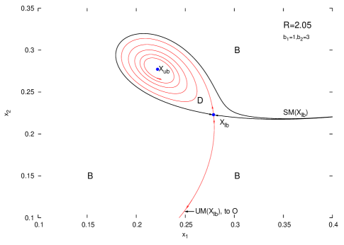
Figure 2: For a value of $R$ just greater than the first critical value $R=R_{sn}=2$, the phase portrait is a familiar one in which the boundary of the basin of attraction of $O$ is likewise the boundary of the basin of attraction of a second, stable equilibrium point $X_{ub}$.

4.1 A ’simple’ basin

For Figure 2 we choose a value $R=2.05$, just slightly greater than the saddle-node critical value. The equilibrium point $X_{ub}$ is stable and has its own basin of attraction, indicated by $D$ in the figure. The remainder of the phase space lies in $B$, the basin of attraction of the origin. The equilibrium point $X_{lb}$ has one stable and one unstable direction. Its stable manifold, $SM(X_{lb})$, forms the common boundary of $D$ and $B$. This picture is similar to that of the simple basin of attraction of §1 in that the basin boundary divides phase space into the sharply distinct regions $B$, where all orbits relaminarize, and $D$ where no orbits relaminarize. It differs in details: the part of the domain $D$ that lies to the right of $X_{lb}$ becomes extremely thin, the two arcs of $SM(X_{lb})$ coming progressively closer to coincidence for progressively larger values of $x_{1}$. It differs also in that the basin boundary is unbounded. Before considering larger values of $R$ we we make some observations about the system near the saddle-node value.

First, consider linearizing the system (2) about $X_{sn}$, the saddle node point, for $R=R_{sn}$. The matrix of linearization (equation 6) is

$$\left(\begin{array}[]{cc}-1/4&-1/4\\ 1/4&1/4\end{array}\right)\approx\left(\begin{array}[]{cc}0&0\\ 1&0\end{array}\right)$$

under similarity transformation. If we were to unfold the singularity at that point, the unfolding would be of Takens-Bogdanov type. Of course we have a system with prescribed nonlinear terms so we do not undertake this unfolding but it is interesting to note that in a far more faithful representation of the pipe-flow problem (see [8]) one is led to this unfolding at the corresponding value $R_{sn}$.

Next note that, despite the unboundedness of $D$, it has a small area. A perturbation of the laminar flow has only a small probability of lying in $D$ and therefore a high probability of relaminarizing.

Finally we note that a hint of ’edge’ behavior exists in this diagram: for values of $x_{1}$ exceeding (say) $0.35$, two initial points near $SM$, one just above the upper arc and the other just below the lower arc, lead to quite different trajectories, although both end up at $O$.

4.2 Homoclinic bifurcation

As $R$ increases further the region $D$ begins to increase in size but a new critical value of $R=R_{h}\approx 2.14$ occurs where a homoclinic bifurcation takes place: the two branches of $SM(X_{lb})$ to the right of $X_{lb}$ seen in Figure 2 coalesce into a single orbit, and $D$ is now bounded by a homoclinic loop. This is depicted in Figure 3. The part of the stable manifold of $X_{lb}$ to the right of this point has now taken the form of an edge as described elsewhere ([9]).

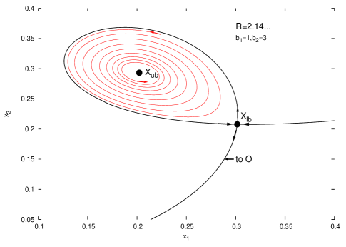
Figure 3: At the second critical value $R=R_{h}=2.14\ldots$, there is a homoclinic bifurcation of phase portraits, depicted here and producing an edge.

Increasing $R$ beyond $R_{h}$ we see (Figure 4) that the domain $D$ is now bounded by a periodic orbit, indicated by $P$ in Figure 4. Both arcs of $SM(X_{lb})$ now have the edge character. The boundary of $B$, the basin of attraction of $O$, is the union of $P$ with $SM(X_{lb})$. The left-hand arc of the latter now coincides with the unstable manifold of the unstable periodic orbit $P$.

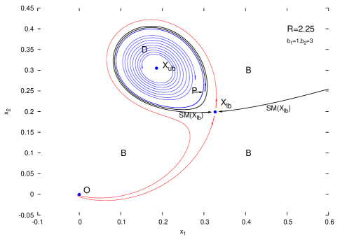
Figure 4: For a slightly larger value of $R$ than that shown in Figure 3, the phase portrait has changed qualitatively. No longer like the familiar picture, there is now an edge, agreeing with the stable manifold of $X_{lb}$. The basin of attraction of $X_{ub}$ is now bounded; its boundary is the periodic orbit $P$.

4.3 Hopf bifurcation

As $R$ is increased further, the basin of attraction of $X_{ub}$ begins to shrink (see Figure 5) and the stability of that point weakens, i.e., the (negative) real parts of the eigenvalues get smaller in absolute value. This culminates in a further bifurcation point $R=R_{bh}$ at which the real parts of the eigenvalues vanish and the domain $D$ evanesces. For $R_{bh}<R<R_{\infty}$, essentially all of the ambient space lies in $B$, i.e., essentially all orbits relaminarize. The only exceptions are those lying on the stable manifold of $X_{lb}$, but these would be sampled with probability zero (see Figure 6). The basin boundary is now a pure edge state.

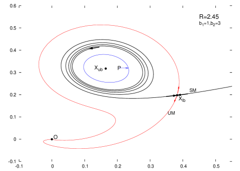
Figure 5: The geometry of the phase portraits is qualitatively the same as in Figure 4. The value of $R$ is just less than $R_{bh}=2.5$, at which the stability of $X_{ub}$ changes. The basin of attraction of $X_{ub}$ has shrunk. The complementary region to the basin of attraction of $O$ now consists only of this region (bounded by $P$) and the pair of curves comprising $SM$, the stable manifold of $X_{lb}$.

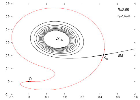
Figure 6: In this figure, $R$ is just greater than $R_{bh}=2.5$. The edge, consisting of the stable manifold of $X_{lb}$, is now “pure” in the sense that all orbits except those lying on this set relaminarize.

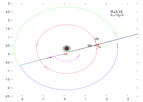
Figure 7: Qualitatively like Figure 6 but for value of $R$ approaching $R_{\infty}$, where $X_{lb}\to\infty$. Three orbits are shown (green,blue,magenta) to indicate that most orbits are similar to the arcs of $UM$.

4.4 A final bifurcation

Finally, for $R>R_{\infty}$, the basin of attraction of the origin is restored to finite size, as in Figure 8, and the simple picture of a basin is restored: the boundary separates orbits that relaminarize from those that do not and there is no edge state. Moreover, as $R$ increases, $X_{lb}\to O$ (like $1/R^{2}$ for large $R$) and therefore the distance from $O$ to $\partial B$ likewise tends to zero (like $1/R^{3}$; cf [3] for this estimate). This is the basic picture of subcritical transition, since perturbations of $O$ may find themselves outside $B$ despite being very small. Figure 9 is qualitatively the same but for a larger value of $R$.

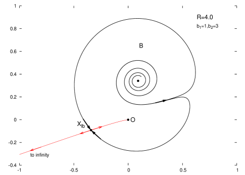
Figure 8: The value of $R$ now exceeds that of a fourth critical point $R_{\infty}=10/3$. The basin of attraction of the origin is now finite. What appears to be a spiral surrounding the equilibrium point $X_{ub}$ (unmarked in this figure) is in fact a pair of spirals very close together. They are better resolved in Figure 9 below.

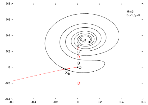
Figure 9: Qualitatively similar to Figure 8. The regions marked $B$ and $D$ are respectively the basin of attraction of $O$ and the region where all orbits tend to $\infty$. The origin of coordinates now lies closer to the basin boundary.

5 Conclusions

That certain features of transition in shear flows can be captured by low-dimensional – even two-dimensional – models is well-known ([4],[10],[2],[3]). The present study adds to these features a picture of an edge state. It confirms the view ([9]) that the edge is a codimension-one invariant set embedded in the basin of attraction of the laminar state. In the present paper the edge state is in fact the stable manifold of the unstable equilibrium point $X_{lb}$. It emerges as an edge state simultaneously with the emergence of a periodic orbit via a homoclinic bifurcation at $R=R_{h}$. This periodic orbit forms the boundary of the basin of attraction of a further stable equilibrium point $X_{ub}$, and the boundary $\partial B$ of the basin of attraction of the origin consists of the union of this periodic orbit with the edge in the interval $R_{h}<R<R_{bh}$.

A similar result appears in a four-dimensional model ([7]), wherein an edge state likewise makes an appearance via a homoclinic bifurcation. In that study, as in this one, simultaneously with the appearance of the edge state there appears a periodic orbit $P$. In that case, whereas the equilibrium point $X_{ub}$ is unstable, there is a stable periodic orbit $Q$ with basin of attraction $D$. The boundary $\partial D$ of $D$ contains the periodic orbit $P$, which is a relative attractor: it is unstable but is an attractor for orbits lying in $\partial D$. In [7] an interpretation of the edge was offered as a pair of surfaces bounding an exquisitely narrow gap containing points of $D$. However, in view of the results of the present paper, it seems more likely that the edge, there also, is a single surface: the stable manifold of the equilibrium point $X_{lb}$, separating $B$ into two regions. In the nine-dimensional model of [9] the basin boundary similarly contains a chaotic, invariant subset. In all these cases orbits starting near the basin boundary may well participate in the dynamics of such invariant subsets – and therefore be quite complex – for a while before relaminarizing. In the higher-dimensional cases the complexity can be heightened if the invariant sets in question are highly convoluted.

In the present model there is a final critical value $R_{\infty}$ of the parameter beyond which the edge state has disappeared and the geometrical structure of phase space is consistent with the interpretation of a permanent, subcritical transition away from the laminar state. It is of course not clear that this result extends beyond this simple model.

References

- [1] M. Avila, A.P. Willis, and B. Hof. On the transient nature of localized pipe flow turbulence. JFM, 646:127–136, 2010.
- [2] J.S. Bagget, T.A. Driscoll, and L.N. Trefethen. A mostly linear model of transition to turbulence. Phys. Fluids, 7:883, 1995.
- [3] J.S. Bagget and L.N. Trefethen. Low-dimensional models of subcritical transition to turbulence. Phys. Fluids, 9:1043–1053, 1997.
- [4] O. Dauchot and P. Manneville. Local versus global concepts in hydrodynamic stability theory. Jour. Phys. II France, 7:371–389, 1997.
- [5] B. Eckhardt. Turbulence transition in pipe flow: some open questions. Nonlinearity, 21:T1–T11, 2008.
- [6] Siegried Grossmann. The onset of shear flow turbulence. Rev. Mod. Phys., 72(2):603–618, 2000.
- [7] N. Lebovitz. Shear-flow transition: the basin boundary. Nonlinearity, 22:2645–2655, 2009.
- [8] F. Mellibovsky and B. Eckhardt. Takens-bogdanov bifurcation of traveling wave solutions in pipe flow. arXiv, (1002.1640), 2010.
- [9] J.D. Skufca, J.A. Yorke, and B. Eckhardt. Edge of chaos in a parallel shear flow. Phys. Rev. Lett., 96:174101, 2006.
- [10] A. Trefethen, S. Trefethen, S. Reddy, and T. Driscol. Hydrodynamic stability without eigenvalues. Science, 261(5121):578–584, 1993.