Quantum effect on luminosity-redshift relation

Abstract

There are many different proposals for a theory of quantum gravity. Even leaving aside the fundamental difference among theories such as the string theory and the non-perturbative quantum gravity, we are still left with many ambiguities (and/or parameters to be determined) with regard to the choice of variables, the choice of related groups, etc. Loop quantum gravity is also in such a state. It is interesting to search for experimental observables to distinguish these quantum schemes. This paper investigates the loop quantum gravity effect on luminosity-redshift relation. The quantum bounce behavior of loop quantum cosmology is found to result in multivalued correspondence in luminosity-redshift relation. And the detail multivalued behavior can tell the difference of different quantum parameters. The inverse volume quantum correction does not result in bounce behavior in this model, but affects luminosity-redshift relation also significantly.

I Introduction

In recent years, we witnessed rapid development in quantum gravity theories, especially in the string theory and the loop quantum gravity theory. Both of them have produced many important results. For loop quantum gravity, area and volume operators have been quantized rovelli95 ; ashtekar97 ; ashtekar98a ; thiemann98 . The entropy of black holes rovelli96 can be calculated from statistical mechanics. In addition, as a successful application of loop quantum gravity to cosmology, loop quantum cosmology (LQC) has an outstanding result—replacing the big bang spacetime singularity of cosmology with a big bounce bojowald01 . LQC also gives a quantum suppression of classical chaotic behavior near singularities in the Bianchi-IX models bojowald04a ; bojowald04b . Furthermore, it has been shown that non-perturbative modification of the matter Hamiltonian leads to a generic phase of inflation bojowald02 ; date05 ; xiong1 . We also know that there are many alternative ways for quantum gravity, including the string theory and non-perturbative quantum gravity. Within non-perturbative quantum gravity only, we have also many choices for quantization, with freedom in, for example, the choice of variables and the choice of the related groups. Thus any contribution from experimental observation would be all the more valuable.

In cosmology, the data accumulated are plenty, actually more than what theory can explain. Among the observations, the luminosity-redshift relation of type Ia supernovae (SNIa) suggests that the universe has entered a phase of accelerating expansion and that the universe is spatially flat perlmutter99 . It is thus interesting to see if we can use this observable to verify any quantum gravity schemes, or use a gedanken experiment to test the different behaviors of different schemes. This is the topic of this paper. Based on the effective LQC theory, we look into the effect of quantum correction on the luminosity-redshift relation, and test the different choices involved in LQC, which have been causing ambiguity. Classically, scalar field is used to explain dark matter/energy, and the scalar field model fits the experiment data well matos00 . Therefore we use this model as the classical reference for investigating the quantum effects.

This paper is organized as follows. The next section, we give a brief review of effective LQC theory. In this paper we consider only the holonomy correction and the inverse volume correction. In Sec.III, we use a massless scalar field to model the dark matter/energy, and derive the classical luminosity-redshift relation of this model. For comparison with LQC, we adopt the formalism of effective LQC to express this classical dynamics. In Secs.IV and V, we study the quantum effects, paying much attention to the $l$-parameter in the $\bar{\mu}$ scheme. We conclude the paper in the last section. Through out this paper we adopt $c=G=\hbar=1$ which results in the Hubble constant $H_{0}\approx 1.2\times 10^{-61}$.

II framework of effective LQC

Based on the assumptions of cosmological principle and that the universe is spatially flat, the metric of the related spacetime is described by FRW metric

$$ds^{2}=-dt^{2}+a^{2}(dx^{2}+dy^{2}+dz^{2}),$$ (1)

where $a$ is the scale factor of the universe, which only depends on $t$ due to homogeneity of our universe. The classical Hamiltonian for the system we considered in this paper is given by

$$H_{cl}=-\frac{3}{8\pi\gamma^{2}}\sqrt{p}c^{2}+H_{M}\left(p,\phi\right).$$ (2)

Here we have adopted the Ashtekar variables in loop quantum gravity. The phase space is spanned by the generalized coordinates $c=\gamma\dot{a}$ and the generalized momentum $p=a^{2}$. $\gamma=0.2375$ is the Barbero-Immirzi parameter. $H_{M}$ denotes the Hamiltonian of the matter part and $\phi$ denotes the matter field. Together with the Poisson bracket for the gravity part, which is defined for any two functions $f$ and $g$ on phase space as

$$\{f,g\}:=\frac{8\pi\gamma}{3}\left(\frac{\partial f}{\partial c}\frac{\partial g}{\partial p}-\frac{\partial f}{\partial p}\frac{\partial g}{\partial c}\right),$$ (3)

we can get the corresponding canonical equations.

Correspondingly, the effective Hamiltonian in LQC is given by ashtekar06

$$H_{eff}=-\frac{3}{8\pi\gamma^{2}\bar{\mu}^{2}}\sqrt{p}\sin^{2}\left(\bar{\mu}c\right)+H_{M}\left(p,\phi\right).$$ (4)

If we consider the inverse volume quantum correction, $H_{M}$ will change correspondingly. We will describe more in Sec.V. The variable $\bar{\mu}$ corresponds to the dimensionless length of the edge of the elementary loop and is given by

$$\bar{\mu}=\xi p^{-l},$$ (5)

where $\xi>0$ is a constant and depends on the particular scheme in the holonomy corrections. According to the idea of area quantization and the requirement of area gap, we have hrycyna09

$$\xi^{2}=2\sqrt{3}\pi\gamma l_{p}^{2},$$ (6)

where $l_{p}=1$ is the Planck length. $l$ is an ambiguous parameter in LQC. Considerations of the lattice states place an restriction that $l\in(0,0.5]$ resl1 . The anomaly cancellation and the positivity of the graviton’s effective mass requires $l\in[0.1319,2.5]$ resl2 . But we are still not able to fix this ambiguity parameter theoretically. Later in this paper we will test the influence of different values of $l$ on the luminosity-redshift relation.

III Classical scalar field model

In this section we will investigate the classical dynamics of the universe using scalar field to model the dark matter/energy. The universe is nearly homogeneous and isotropic, with roughly $4\%$ of the matter content being ordinary matter, $22\%$ being cold dark matter and $74\%$ being dark energy. Until now, we do not know the nature of the cold dark matter and the dark energy, here we use a massless scalar field to model the cold dark matter and the dark energy, and ignore the ordinary matter part. The Hamiltonian of the classical scalar field model is

$$H_{cl} = -\frac{3}{8\pi\gamma^{2}}c^{2}\sqrt{p}+\frac{p_{\phi}^{2}}{2p^{3/2}}+p^{\frac{3}{2}}V(\phi),$$ (7)

where $p_{\phi}$ is the conjugate momentum of the free massless scalar field $\phi$. Following matos00 we take

$$V=V_{0}e^{-\sqrt{\frac{16\pi}{\lambda}}\phi},$$ (8)

where $V_{0}$ is some constant. The equations of motion in this classical case are given by Hamilton’s equations:

$$\dot{c} = -\frac{1}{2\gamma\sqrt{p}}c^{2}-2\pi\gamma\frac{p^{2}_{\phi}}{p^{5/2}}+4\pi\gamma V_{0}p^{\frac{1}{2}}e^{-\sqrt{\frac{16\pi}{\lambda}}\phi},$$

$$\dot{p} = \frac{2}{\gamma}c\sqrt{p},$$

$$\dot{\phi} = p^{-3/2}p_{\phi},$$

$$\dot{p_{\phi}} = \sqrt{\frac{16\pi}{\lambda}}V_{0}p^{\frac{3}{2}}e^{-\sqrt{\frac{16\pi}{\lambda}}\phi}.$$

The Friedmann equation reads

$$H^{2}=\frac{8\pi}{3}\rho,$$ (9)

where $\rho=\frac{\dot{\phi}^{2}}{2}+V(\phi)$. The exact solution to the model described above is

$$a = \left(\frac{t}{\bar{t}}\right)^{\lambda},$$ (10)

$$\phi = \sqrt{\frac{1}{4\pi\lambda}}\ln a,$$ (11)

with $\bar{t}=\sqrt{\frac{\lambda(3\lambda-1)}{8\pi V_{0}}}$. And the parameter of the state equation is $\omega=\frac{2}{3\lambda}-1$. We will see in the following that $\omega$ is a negative constant, to be consistent with the property of cold dark matter and dark energy, for which the equation of state parameters are 0 and -1 respectively.

The luminosity distance is a way of expressing the amount of light received from a distant object. When we receive a certain flux from an object, we can calculate the luminosity distance between us and the object, assuming the inverse square law for the reduction of light intensity with distance holds. Because of the expansion of the universe, the number of photons in unit volume of a sphere shell will decrease $\propto\frac{a_{0}}{a}=(1+z)$, where $z$ is the redshift factor. Considering the cosmological redshift effect, the individual photons will lose energy $\propto(1+z)$. Based on the above inverse square law assumption, we get luminosity distance

$$d_{L}=a_{0}(1+z)\int_{0}^{t}\frac{dt}{a(t)}.$$ (12)

Given the above exact solution, we have

$$d_{L}=\frac{(1+z)\lambda}{H_{0}(1-\lambda)}\left[1-(1+z)^{1-\frac{1}{\lambda}}\right].$$ (13)

According to the astronomical convention, we adopt the logarithmic measure of the luminosity instead of luminosity itself in presenting our result,

$$\mu=5\log_{10}d_{L}-286.4,$$ (14)

here -286.4 comes from our units $c=G=\hbar=1$ . Using Eq.(13) in the above equation, we get

$$\mu=43.17+5\log_{10}\left\{{\frac{\lambda(1+\lambda)}{1-\lambda}\left[1-(1+z)^{1-\frac{1}{\lambda}}\right]}\right\}.$$ (15)

Fitting $\lambda$ in this equation to the experimental data reported in reiss04 , we get $\lambda=2.38$ which results in the parameter of the state equation $\omega=-0.72$. For cold dark matter and dark energy the total pressure can be expressed as

$$P=P_{M}+P_{E}=-\rho_{E}=-0.72\rho,$$ (16)

where subfix $M$ means the cold dark matter, and $E$ means dark energy. In the above equation, we have used $\omega_{M}=0$ and $\omega_{E}=-1$. Thus our fitted result $\omega=-0.72$ is consistent with roughly $74\%$ of our universe being dark energy. As Fig.1 shows, the resulted line lies closely with the experimental data.

Figure 1: Fit of the theoretical luminosity-redshift relation (line), as described in Eq.(15), to the experimental data for type-I supernova reported in reiss04 (solid circles).

In order to investigate the quantum effects, we turn to the quantum region of the universe. We introduce a parameter $\alpha:=\frac{\rho_{M}}{\rho_{c}}$, the ratio between the matter density and the quantum critical density ($\rho_{c}=\frac{\sqrt{3}}{16\pi^{2}\gamma^{3}}\approx 0.82$), to indicate how close we are to the quantum region. Given $\alpha$, we can determine $\rho_{M}$ and then the time $t$ which gives all the dynamical variables according to the above exact solution (10). In the rest of this paper, we regard $t$ as the “present time”, to investigate the quantum effects on luminosity-redshift relation. Since the constant of $286.4$ is irrelevant to us for comparing with the classical luminosity-redshift relation, we will ignore it in the following, and will define the luminosity-redshift relation simply as

$$\mu=5\log_{10}d_{L}.$$ (17)

IV holonomy quantum correction of the scalar field model

Based on the effective description of quantum dynamics for LQC as described in Sec.II, the Hamiltonian can be written as ashtekar06 ; bentivegna08

$$H_{eff}^{hc} = -\frac{3}{8\pi\gamma^{2}\bar{\mu}^{2}}p^{1/2}\sin^{2}(\bar{\mu}c)+\frac{p_{\phi}^{2}}{2p^{3/2}}+p^{\frac{3}{2}}V_{0}e^{-\sqrt{\frac{16\pi}{\lambda}}\phi},$$ (18)

for the holonomy quantum correction of the scalar field model considered in this work. In the limit of $\bar{\mu}\rightarrow 0$, this Hamiltonian reduces to the standard classical one. The dynamical equations are given by

$$\dot{c} = -\frac{1}{2\gamma\bar{\mu}^{2}\sqrt{p}}\sin^{2}(\bar{\mu}c)+2l\frac{1}{\gamma\bar{\mu}\sqrt{p}}\sin(\bar{\mu}c)\cos(\bar{\mu}c)c$$ (19)

$$- 2l\frac{1}{\gamma\bar{\mu}^{2}\sqrt{p}}\sin^{2}(\bar{\mu}c)-2\pi\gamma p_{\phi}^{2}p^{-\frac{5}{2}}+4\pi\gamma V_{0}p^{\frac{1}{2}}e^{-\sqrt{\frac{16\pi}{\lambda}}\phi},$$

$$\dot{p} = \frac{2}{\gamma}\frac{\sqrt{p}}{\bar{\mu}}\sin(\bar{\mu}c)\cos(\bar{\mu}c),$$ (20)

$$\dot{\phi} = p^{-\frac{3}{2}}p_{\phi},$$ (21)

$$\dot{p}_{\phi} = \sqrt{\frac{16\pi}{\lambda}}V_{0}p^{\frac{3}{2}}e^{-\sqrt{\frac{16\pi}{\lambda}}\phi}.$$ (22)

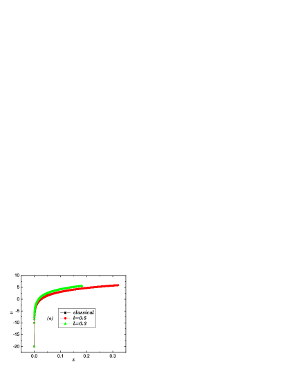
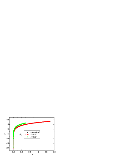
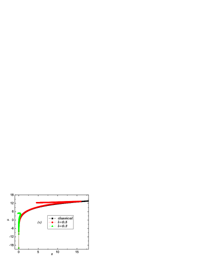
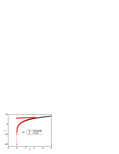
Figure 2: Comparison of the luminosity-redshift relation in the classical scenario and in the holonomy quantum correction scenario. The corresponding parameters $\alpha$ are 0.0001 in (a), 0.001 in (b), 0.01 in (c), and 0.1 in (d). The holonomy quantum correction gives a multi-valued luminosity-redshift relation.

Following the above classical considerations, we adopt the initial condition $p_{\phi}(0)$, $p(0)$ and $\phi(0)=0$ from the classical scenario. Then $H_{hc}=0$ is used to determine $c(0)$. Fig.2 shows the resulted luminosity-redshift relations for (a) $\alpha=0.0001$, (b) $0.001$, (c) $0.01$, and (d) $0.1$. We can see that quantum corrections with different parameters $l$ gives different luminosity-redshift behaviors. As is clear in Fig.2 (a-c), for larger $l$, it takes a larger $\alpha$ for the quantum effects to be visible. In (d), the quantum corrected universe with $l=0.3$ does not admit $\rho_{M}\leq 0.1\rho_{c}$, so it is left out from this panel. The most interesting result is that the quantum correction leads to a multi-valued luminosity-redshift relation. This multi-valued behavior is actually a result of the quantum bounce when the universe becomes very small. So this multi-valued behavior is a common result for all quantum bounce cosmology models. We expect that the quantum effects can be distinguished through luminosity-redshift relation if we can observe objects far enough. In addition, different values of quantum parameter $l$ give different quantum bounce behaviors: for smaller $l$, the luminosity-redshift Relation turns around at smaller $z$. Thus we conjecture that the luminosity-redshift relation can be used to fix $l$.

V The inverse volume correction of the scalar field model

If we consider the inverse volume correction in LQC, the effective Hamiltonian can be written as bojowald02a ; bojowald02b ; tsujikawa04

$$H_{eff}^{iv}=-\frac{3}{8\pi\gamma^{2}}c^{2}\sqrt{p}+\frac{1}{2}\frac{D(q)}{p^{3/2}}p_{\phi}^{2}+p^{\frac{3}{2}}V_{0}e^{-\sqrt{\frac{16\pi}{\lambda}}\phi}.$$ (23)

Here $D(q)=(\frac{8}{77})^{6}q^{3/2}\{7[(q+1)^{11/4}-|q-1|^{11/4}]-11q[(q+1)^{7/4}-\text{sgn}(q-1)|q-1|^{7/4}]\}^{6},q=p/p_{*}$, and $p_{*}$ is the scale parameter for the inverse volume correction to take place. With Eq.(23), we investigate the effect of the inverse volume correction on the luminosity-redshift relation, and compare it with the effect of the holonomy correction. In the classical cosmology, the scale factor $a=\sqrt{p}$ has no direct physical meaning. We can always rescale it to set the value of $a$ at present time to 1. But in loop quantum cosmology, especially when we consider the inverse volume correction, the scale factor has important consequences. When its value is roughly the Planck length $p_{*}\approx l_{p}^{2}$, the inverse volume correction will take place. The corresponding dynamical equations are

$$\dot{c} = -\frac{1}{2\gamma\sqrt{p}}c^{2}+\frac{4\pi\gamma}{3p_{*}}\frac{dD(q)}{dq}p_{\phi}^{2}p^{-\frac{3}{2}}$$

$$- 2\pi\gamma D(q)p_{\phi}^{2}p^{-\frac{5}{2}}+4\pi\gamma V_{0}p^{\frac{1}{2}}e^{-\sqrt{\frac{16\pi}{\lambda}}\phi},$$

$$\dot{p} = \frac{2}{\gamma}c\sqrt{p},$$

$$\dot{\phi} = D(q)p^{-3/2}p_{\phi},$$

$$\dot{p_{\phi}} = \sqrt{\frac{16\pi}{\lambda}}V_{0}p^{\frac{3}{2}}e^{-\sqrt{\frac{16\pi}{\lambda}}\phi},$$ (24)

where $\frac{dD(q)}{dq}=(\frac{8}{77})^{6}\frac{3}{2}\sqrt{q}\{7[(q+1)^{11/4}-|q-1|^{11/4}]-11q[(q+1)^{7/4}-\text{sgn}(q-1)|q-1|^{7/4}]\}^{6}+(\frac{8}{77})^{6}q^{3/2}6\{7[(q+1)^{11/4}-|q-1|^{11/4}]-11q[(q+1)^{7/4}-\text{sgn}(q-1)|q-1|^{7/4}]\}^{5}\{\frac{33}{4}[(q+1)^{7/4}-\text{sgn}(q-1)|q-1|^{7/4}]-\frac{77}{4}q[(q+1)^{3/4}-|q-1|^{3/4}]\}$. Combining the Hamiltonian constraint with the above dynamical equations, we can get the Friedman equation as

$$\left(\frac{\dot{a}}{a}\right)^{2}=\frac{8\pi}{3}(\frac{\dot{\phi}^{2}}{2D}+V).$$ (25)

Due to the exponential form of our scalar potential $V$, $\dot{a}$ will never vanish, which means we can not get quantum bounce with this inverse volume correction. On the other hand, we will see the luminosity-redshift relation can also distinguish this quantum correction from classical behavior. We take the same procedure as in the case of holonomy correction to test this quantum effect on luminosity-redshift relation. Compared with the classical scenario, the resulted luminosity redshift relations are plotted in Fig.3. Different from the holonomy quantum correction, the quantum effects take place in smaller universe, roughly $\rho_{M}=0.01\rho_{c}$. Although this may depend on model, the interesting point is the luminosity-redshift relation as an observable can distinguish the quantum effect from classical behavior.

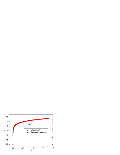
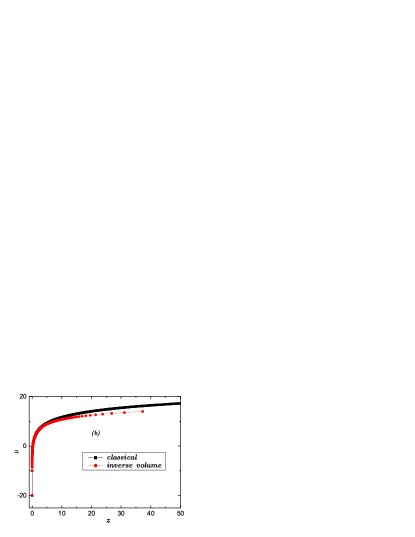
Figure 3: Comparison of the luminosity-redshift relation in classical scenario and the inverse volume quantum correction scenario, for $\alpha=0.001$ in (a) and $0.01$ in (b). Compared with the holonomy quantum correction, the inverse volume quantum correction takes place at smaller universe in our model.

VI comments and conclusions

There are currently different proposals for a theory of quantum gravity, including the string theory and the loop quantum gravity theory, among others. They all pass the check of self-consistency. Even in the loop quantum gravity theory alone, there are many ambiguities that we do not know the way to eliminate. To a large extent, this situation results from the lack of association with experimental data. On the other hand, there are plenty of experiment data in cosmology awaiting satisfactory explanation. For example, we have yet to have a consistent theory to explain the accelerating expansion of the universe at the present age.

In this paper we use the luminosity-redshift relation to test LQG effects. We find this relation to be capable of revealing the quantum effects and fixing the quantum parameters. LQC predicts a multi-valued luminosity-redshift relation, as a result of the quantum bounce behavior. The exact shape of the relation can be used to fix quantum parameters in LQC. We can also distinguish the inverse volume quantum correction from the classical picture. Although some of the predictions made in this paper can not yet be tested using the experiment data available, it is a good gedanken experiment at least, to study the ambiguities involved in LQC and how they can be eliminated. Certainly, this paper touches merely a small part of the problem with ambiguity in LQC, yet our results show that the quantum bounce behavior is possibly observable through the multi-valued shape of luminosity-redshift relation.

- (1) C. Rovelli and L. Smolin, Nucl. Phys. B 442, 593 (1995).
- (2) A. Ashtekar and J. Lewandowski, Class. Quant. Grav. 14, A55 (1997).
- (3) A. Ashtekar and J. Lewandowski, Adv. Theor. Math. Phys. 1, 388 (1998).
- (4) T. Thiemann, J. Math. Phys. 39, 3372 (1998).
- (5) C. Rovelli, Phys. Rev. Lett. 77, 3288 (1996).
- (6) M. Bojowald, Phys. Rev. Lett. 86, 5227 (2001).
- (7) M. Bojowald, Phys. Rev. Lett. 92, 071302 (2004).
- (8) M. Bojowald, Class. Quantum Grav. 21, 3541 (2004).
- (9) M. Bojowald, Phys. Rev. Lett. 89, 261301 (2002).
- (10) G. Date and G. Hossain, Phys. Rev. Lett. 94, 011301 (2005).
- (11) Hua-Hui Xiong and Jian-Yang Zhu, Phys. Rev. D 75, 084023 (2007).
- (12) S. Perlmutter et al., Astrophys. J. 517, 565 (1999); A.G. Riess et al., Astron. J. 116, 1009 (1998).
- (13) T. Matos, F. Guzman, and L. Urena-Lopez, Class. Quantum Grav. 17, 1707 (2000).
- (14) A. Ashtekar, T. Pawlowski, and P. Singh, Phys. Rev. D 73, 124038 (2006); 74, 084003 (2006).
- (15) O. Hrycyna, J. Mielczarek, and M. Szydlowkski, Gen. Relativ. Gravit. 41, 1025 (2009).
- (16) M. Bojowald, Gen. Relativ. Gravit. 38, 1771 (2006); 40, 2659 (2008).
- (17) M. Bojowald and G. M. Hossain, Phys. Rev. D 77, 023508 (2008).
- (18) A. Riess, et al., ApJ 607, 665 (2004).
- (19) E. Bentivegna and T. Pawlowski, Phys. Rev. D 77, 124025 (2008).
- (20) M. Bojowald, Phys. Rev. Lett. 89, 261301 (2002).
- (21) M. Bojowald, Class. Quantum Grav. 19, 5113 (2002).
- (22) S. Tsujikawa, P. Singh and R. Maartens, Class. Quantum Grav. 21, 5767 (2004).