Spectral Transformation Algorithms for Computing Unstable Modes of Large Scale Power Systems

ABSTRACT: In this paper we describe spectral transformation algorithms for the computation of eigenvalues with positive real part of sparse nonsymmetric matrix pencils $(J,L)$, where $L$ is of the form $\pmatrix{M&0\cr 0&0}$. For this we define a different extension of Möbius transforms to pencils that inhibits the effect on iterations of the spurious eigenvalue at infinity. These algorithms use a technique of preconditioning the initial vectors by Möbius transforms which together with shift-invert iterations accelerate the convergence to the desired eigenvalues. Also, we see that Möbius transforms can be successfully used in inhibiting the convergence to a known eigenvalue. Moreover, the procedure has a computational cost similar to power or shift-invert iterations with Möbius transforms: neither is more expensive than the usual shift-invert iterations with pencils. Results from tests with a concrete transient stability model of an interconnected power system whose Jacobian matrix has order 3156 are also reported here.

KEY WORDS: eigenvalues, stability, Möbius transforms, generalized eigenvalues

RESUMO: Neste artigo, descrevemos algoritmos baseados em transformações espectrais para computação de autovalores com parte real positiva de pencils de matrizes esparsas e não simétricas, $(J,L)$, em que $L$ é da forma $\pmatrix{M&0\cr 0&0}$. Para isso definimos uma extensão das transformacões de Möbius a pencils que inibe a atuação do autovalor infinito sobre as iterações. Esses algoritmos usam uma técnica de precondicionamento dos vetores iniciais via transformadas de Möbius que junto com iterações tipo potência inversa com shift aceleram a convergência para os autovalores desejados. Vemos também que as transformadas de Möbius podem ser usadas com sucesso no processo de inibir a convergência para um autovalor já conhecido. Além disso, esse procedimento tem um custo computacional semelhante ao custo computacional de iterações tipo potência ou potência inversa com shift: tão caro como iterações tipo potência inversa com shift aplicadas em pencils. São também apresentados aqui resultados de testes com um modelo prático para o problema de estabilidade transiente de um sistema de potência interconectado, cuja matriz jacobiana é de ordem 3156.

PALAVRAS-CHAVE: autovalores, estabilidade, transformações de Möbius, autovalores generalizados

1991 Mathematics Subject Classification: 65F, 93D

1 Introduction

The power system eletromechanical stability problem can be described by a nonlinear system of differential and algebraic equations

$$\left\{\begin{array}[]{ll}\dot{x}=f(x,y)\\ 0=g(x,y),\end{array}\right.$$

where x, the state vector, contains the dynamic variables and y, the algebraic variables. After linearization around a system operating point ($x_{0},y_{0}$), i.e, ($x_{0},y_{0}$) such that f($x_{0},y_{0}$) = 0, equation (1.1) becomes

$$\pmatrix{\Delta\dot{x}\cr 0}=\pmatrix{J_{1}&J_{2}\cr J_{3}&J_{4}}\pmatrix{\Delta x\cr\Delta y}.$$

By eliminating the vector $\Delta y$ in (1.2) we obtain

$$\Delta\dot{x}=A\Delta x,$$

where $A=J_{1}-J_{2}J_{4}^{-1}J_{3}$ represents the system state matrix, whose eigenvalues provide information about the singular point local stability of the non-linear system. The symbol $\Delta$ used to represent an incremental change from a steady-state value will be omitted from now on.

By a classical result of ODE theory, the local stability of the system (1.1) can be predicted from the system (1.3). If $A$ is diagonalizable the solution of (1.3) is a sum of vectors of the type $e^{\lambda_{i}t}v_{i}$, where $v_{i}$ is an eigenvector associated with the eigenvalue $\lambda_{i}$. Thus, if all eigenvalues have negative real part, the solution decays to zero and in this case, the system is called stable. For an eigenvalue with positive real part, the absolute value of this expression increases in time and the system is unstable — these eigenvalues are called unstable modes. Eigenvalues with null real part give rise to oscillation, which never disappears. Also, eigenvalues with negative real part and non-zero imaginary part, but with small ratio between the real and imaginary parts, cause an oscillation which takes a long time to disappear — these are the low damped modes of the system. In the power system stability problem, we consider a mode $\lambda$ to be low damped if $|Re\,\lambda|<0.02|Im\,\lambda|$. In this paper, we search for algorithms which solve the local stability problem (1.1) by computing eigenvalues: we search for the eigenvalues of $A$ with positive real part. The state matrices $A$ are real, non-symmetric and dense, usually too large for the computation of eigenvalues by the QR method. On the other hand, the Jacobian matrices $J$ are sparse and linear systems with $J$ may be solved by variants of Gaussian elimination. The eigenvalue problem for A,

$$Ax=\lambda x,$$

can be stated equivalently in terms of the Jacobian matrix $J=\pmatrix{J_{1}&J_{2}\cr J_{3}&J_{4}}$ so that

$$\pmatrix{J_{1}&J_{2}\cr J_{3}&J_{4}}\pmatrix{x\cr y}=\lambda\pmatrix{x\cr 0}.$$

or, in matrix notation,

$$Jz=\lambda Lz,$$

where $L=\pmatrix{I&0\cr 0&0}$ is the singular diagonal matrix with 1 (resp. 0) at diagonal entries related to state (resp. algebraic) variables and $z=\pmatrix{x\cr y}$ is an eigenvector of $(J-\lambda L)$. Since $z\neq 0$, $\lambda$ is said to be an eigenvalue of the pencil $(J,L)=\{J-aL|a\in{C}\}$. A possible approach to search for unstable modes is to use the shift-invert transform

$$(J-\lambda_{k}L)z_{k+1}=Lz_{k},$$

with initial shifts on the imaginary axis [16]. Although in [16] the problem is not described as the generalized eigenvalue problem (1.6), the system (1.7) is solved in order to implicitly calculate $(A-\lambda I)^{-1}x_{k}$ — in the authors words, they make use of the augmented system associated to $J$ to shift-invert the state matrix $A$. Other methods like subspace iteration and Arnoldi methods were also adapted to augmented systems and some results of their applicability in power systems are reported in [24]. The use of the Cayley transform technique in order to find rightmost eigenvalues of a non-symmetric matrix was probably first reported in 1987 at the IEEE PICA Conference. There, Uchida and Nagao proposed to search for the biggest eigenvalues in absolute value of $S=(A+hI)(A-hI)^{-1}$, $h>0$ to detect unstable modes of the state matrix $A$ of a power system [23]. There, however, the matrix-vector multiplication $Sv$ was performed in a rather innefficient way. In [1], this operation was better implemented and the Cayley transform was extended in two different ways, described in detail in §2, in order to solve the power system stability problem, given as a generalized eigenvalue problem $Jz=\lambda Lz$, where $J$ is not symmetric and $L$ is diagonal with elements 1 or 0 along the diagonal. The use of the Cayley transform technique to find rightmost eigenvalues of the problem $Jx=\lambda Lx$, for non-symmetric $J$ and $L=\pmatrix{M&0\cr 0&0}$, is also found in Computational Fluid Dynamics [6], [7]; an overview of this technique in several areas is [17]; also, in ARPACK [14], Arnoldi iterations can be performed with Cayley transforms. All these references make use of the extension $(J,L)\mapsto(J-\sigma L)^{-1}(J+\overline{\sigma}L)$, which is one of the two extensions of the Cayley transform analysed in [1], which turns out not to be the best for the problem of interest. Indeed, this extension requires a non-obvious strategy to control instability caused by the spurious eigenvalue at infinity of the generalized eigenvalue problem, in the case when $L$ is singular. Here we propose to consider another extension: $(J,L)\mapsto(J+\overline{\sigma}L)(J-\sigma L)^{-1}$. For this matrix the eigenspace associated with the eigenvalues that correspond to finite eigenvalues of the original problem is just the range of $L$, as we shall see in §2. Thus, the spurious eigenvalue is handled by keeping iterations in this space. In the power system stability problem, the range of $L$ is the set of vectors with coordinates related to algebraic variables equal to zero. In the case $L=\pmatrix{M&0\cr 0&0}$ is a matrix of order $n+m$, where $M$ is a $n\times n$ positive definite matrix, as in [6], the space is just the set of vectors with the last m coordinates equal to zero. In §2, we introduce Möbius transforms (a generalization of the Cayley transforms) for the generalized non-symmetric eigenvalue problem. Möbius transforms can be used to precondition random initial vectors as well as to inhibit the convergence to eigenvalues already found (much like a deflation technique), at a computational cost not more expensive than a shift-invert iteration with pencils. The application of polynomial filters to vectors in the computation of eigenvalues of sparse non-symmetric matrices has been the subject of several papers [21], [18], [5]. We will see that Möbius transforms can be seen as the action of a rational function filter which gives infinite and zero weights to two arbitrary points in the complex plane. These techniques are presented in §3 together with two algorithms based on them. Finally, in §4 we apply four methods to the computation of the unstable modes of a pencil $(J,L)$, where $J$ is a sparse matrix of order 3156 and $L$ is diagonal with elements 1 or 0 on the diagonal, of rank 790: the algorithms we suggest, an implementation of the Arnoldi method (ARPACK) and an implementation of the Arnoldi method with acceleration by Chebyshev polynomials (ARNCHEB), both applied on the extension of a Cayley transform introduced here and a subspace iteration applied on the pencil $(J,L)$.

2 The Generalized Eigenvalue Problem and Möbius Transforms

The Möbius transforms are complex functions

$$c_{k,\alpha,\beta}:{C}\cup\{\infty\} \longrightarrow {C}\cup\{\infty\}$$

$$s \mapsto k\,\frac{s+\overline{\beta}}{s-\alpha}$$

where $\alpha+\overline{\beta}\neq 0$. They are conformal mappings which map lines and circumferences to lines or circumferences. When $k=1$ and $\beta=\alpha$, with $Re\,\alpha\neq 0$, these functions are the so called Cayley transforms, which map the semiplane $\{z|Re\,z>0\}$ to $\{z;|z|>1\}$ ($\{z;|z|<1\}$) if $Re\,\alpha>0$ ($Re\,\alpha<0$). Möbius transforms can be defined in the space of square matrices in a analogous way: given a square matrix $A$ and $\alpha$ not in $\lambda(A)$ (the spectrum of $A$) then $k(A+\overline{\beta}I)(A-\alpha I)^{-1}$ is a matrix whose spectrum is $\{k(\lambda+\overline{\beta})(\lambda-\alpha)^{-1};\lambda\in\lambda(A)\}$. However, the extension of these transforms to pencils $(J,L)$ can be done in two ways. The goal of this section is to present the advantages of one extension over the other in the application to the power system stability problem. Also, we will see that multiplication of a Möbius transform against a vector requires no more computations as solving the equation $(J-aL)z=w$, for some (easily computed) scalar $a$. We begin with a lemma that insures that under generic conditions the pencil $(J,L)$ has exactly $n$ eigenvalues, where $n$ is the rank of $L$. Since by the Singular Value Decomposition there are unitary matrices $U,V$ such that $U(J-aL)V^{H}=\hat{J}-a\Sigma$, $\Sigma=diag(d_{1},...,d_{n},0,...,0)$ for appropriate real numbers $d_{i}$ [9], we may suppose without loss that $L=diag(d_{1},...,d_{n},0,...,0)$.

Lemma 21

Let $J=\pmatrix{J_{1}&J_{2}\cr J_{3}&J_{4}}$ and $L=\pmatrix{D&0\cr 0&0}$, where $D$ is a nonsingular diagonal matrix. Then, if $J_{4}$ is nonsingular, $(J-\sigma L)$ is singular if and only if $\sigma$ is an eigenvalue of $D^{-1}A$, where $A=J_{1}-J_{2}J_{4}^{-1}J_{3}$.

Proof: If $J_{4}$ is nonsingular, $A=J_{1}-J_{2}J_{4}^{-1}J_{3}$ can be defined. Now,

$$\pmatrix{J_{1}-\sigma D&J_{2}\cr J_{3}&J_{4}}\pmatrix{x\cr y}=\pmatrix{0\cr 0}\Longleftrightarrow(A-\sigma D)\,x=0\mbox{ and }y=-J_{4}^{-1}J_{3}\,x.$$

Therefore, $(J-\sigma L)$ is singular $\Longleftrightarrow$ $\sigma$ is an eigenvalue of $D^{-1}A$.  

From now on, the non-sigularity of $J_{4}$ will be assumed. Let $\alpha\in{C}$, such that $(J-\alpha L)$ is nonsingular. For $k,\beta\in{C}$, $k\neq 0$ and $\beta\neq-\bar{\alpha}$, let

$$C_{k,\alpha,\beta}=k(J+\bar{\beta}L)(J-\alpha L)^{-1}\mbox{ and }D_{k,\alpha,\beta}=k(J-\alpha L)^{-1}(J+\bar{\beta}L).$$

Notice that these two matrices have the same spectrum. Moreover, they are both extensions of Möbius transforms applied to the pencil $(J,L)$ and the spectrum of $(J,L)$ is related to the spectrum of the two extensions by the relation $s\mapsto k\displaystyle{\frac{s+\overline{\beta}}{s-\alpha}}.$ However, the eigenspaces of both extensions are not the same in general, according to the following propositions whose proofs are left to the reader.

Proposition 22

(a) $z\neq 0$ is an eigenvector of $C_{k,\alpha,\beta}$ associated with $\mu$, $\mu\neq k$, if and only if $Jw=\lambda Lw$, where $w=(J-\alpha L)^{-1}\,z$ and $\lambda=\displaystyle{\frac{k\bar{\beta}+\mu\,\alpha}{\mu-k}}$.

(b) $z\neq 0$ is an eigenvector of $C_{k,\alpha,\beta}$ associated with the eigenvalue $k$ if and only if $L(J-\alpha L)^{-1}z=0$.

Proposition 23

(a) $z\neq 0$ is an eigenvector of $D_{k,\alpha,\beta}$ associated with $\mu$, $\mu\neq k$, if and only if $Jz=\lambda Lz$, where $\lambda=\displaystyle{\frac{k\bar{\beta}+\mu\,\alpha}{\mu-k}}$.

(b) $z\neq 0$ is an eigenvector of $D_{k,\alpha,\beta}$ associated with the eigenvalue $k$ if and only if $Lz=0$.

Thus, the finite eigenvalues of the pencil $(J,L)$ correspond to the eigenvalues of $C_{k,\alpha,\beta}$ or $D_{k,\alpha,\beta}$ that are different from $k$. These eigenspaces are described in the following proposition.

Proposition 24

(a) The eigenspace of $C_{k,\alpha,\beta}$ associated with the eigenvalues different from $k$ is the range of $L$.

(b) The eigenspace of $D_{k,\alpha,\beta}$ associated with the eigenvalues different from $k$ is the range of $(J-\alpha L)^{-1}L$.

Proof: Let $z$ be a vector such that $C_{k,\alpha,\beta}^{H}\,z=kz$. Thus $(J^{H}-\beta L^{H})z=(J^{H}-\bar{\alpha}L^{H})z$ and, since $\beta\neq\bar{\alpha}$, $L^{H}z=0$. Since the eigenspace of $C_{k,\alpha,\beta}$ associated with the eigenvalues different from $k$ is orthogonal to the eigenspace of $C_{k,\alpha,\beta}^{H}$ associated with $k$, that eigenspace is the range of $L$.

The proof of the second part of the proposition is analogous.  

Corollary 25

Let $J=\pmatrix{J_{1}&J_{2}\cr J_{3}&J_{4}}$ a matrix of order $n+m$, where $J_{4}$ is a $m\times m$ nonsingular matrix, and let $L=\pmatrix{M&0\cr 0&0}$, where $M$ is a $n\times n$ nonsingular matrix. Then the eigenspace of $C_{k,\alpha,\beta}$ associated with the eigenvalues different from $k$ is the space of vectors whose last $m$ coordinates are zero.

Since we are interested in calculating eigenvalues of the pencil $(J,L)$ from Möbius transforms, the eigenvalue $k$ of the transform must be treated with special care. The corollary above states that in the case of the power system stability problem, for instance, the invariant subspace $V$ corresponding to the eigenvalues different from $k$ is the set of vectors $v$ that have null coordinates in the positions related to algebraic variables. The iterates of our approximate eigenvectors ought to stay in this subspace, and if the computation of $C_{k,\alpha,\beta}v$ leaves $V$ because of errors due to finite precision arithmetic, we simply project the results back to $V$ by zeroing the appropriate coordinates. The analogous iteration with the Möbius extension $D_{k,\alpha,\beta}$ is not subject to such an easy stabilization procedure, and in this case approximate eigenvectors will frequently converge to the eigenspace associated to $k$, which is of no real interest for the pencil eigenvalue problem. Hence, we will only consider here iterations making use of the extension $C_{k,\alpha,\beta}$.

Now, let $\sigma\in{C}$, with $Re\,\sigma>0$, such that $(J-\sigma L)$ is nonsingular, and consider

$$C_{\sigma}=C_{1,\sigma,\sigma}=(J+\overline{\sigma}L)(J-\sigma L)^{-1}$$

Let $\mu\neq 1$. Then, simple calculations obtain

$$(C_{\sigma}-\mu I)=(1-\mu)I+2\,Re\,\sigma\,L\,(J-\sigma\,L)^{-1}$$

$$(C_{\sigma}-\mu I)^{-1}=\frac{1}{1-\mu}\;[\,I+\frac{2\,Re\,\sigma}{\mu-1}\,L\,(J-\frac{\bar{\sigma}+\mu\sigma}{\mu-1}\,L)^{-1}\,],$$

$$(C_{\sigma}^{-1}-\mu I)^{-1}=\frac{1}{1-\mu}\;[\,I-\frac{2\,Re\,\sigma}{\mu-1}\,L\,(J+\frac{\sigma+\mu\bar{\sigma}}{\mu-1}\,L)^{-1}\,].$$

Thus, the computational cost of applying any of the three matrices in the left-hand side to a vector is equivalent to solving a system $(J-aL)w=z$. Similar results hold for both extensions of Möbius transforms.

The spectra of the pencil $(J,L)$ and of $C_{\sigma}$ are related to each other by the bijective function

$$c_{\sigma}:{C}\cup\{\infty\} \longrightarrow {C}\cup\{\infty\}$$

$$s \mapsto \frac{s+\overline{\sigma}}{s-\sigma}$$

This function maps complex numbers with negative real part onto the unitary circle, pure imaginary ones onto the unitary circumference and those with positive real part onto numbers outside the unitary circle. The search for eigenvalues of largest absolute value of the extension of the Cayley transform thus obtains the unstable modes of the original pencil. Unfortunately, this transformation clusters some eigenvalues very close together, thus affecting adversely the rate of convergence. Therefore, we need techniques to accelerate the convergence to the desired eigenvalues. This is the goal of the next section.

3 A Class of Spectral Algorithms

Two ways of extending Möbius transforms to the pencil $(J,L)$ were described in the previous section. When $L$ is a matrix of order $n+m$ and of the type $\pmatrix{M&0\cr 0&0}$, where $M$ is an $n\times n$ nonsingular matrix, the eigenvectors of the extension $C_{k,\alpha,\beta}$ associated with eigenvalues different from $k$ are the vectors which have zero entries in the last $m$ coordinates. Therefore, in this case, the attraction of the eigenvalue $k$, which corresponds to the infinite eigenvalue of the pencil, can be easily avoided. Now, the power system stability problem, where $M$ is the $n\times n$ identity matrix, has additional features that lead us to explore Möbius techniques. Usually, this problem has several negative real eigenvalues with large modulii, which are mapped to eigenvalues close to $k$: the clustering of eigenvalues substantially reduces the speed of convergence of the power method [9]. In this section we introduce a class of algorithms which use Möbius transforms to precondition vectors, in order to yield more convenient initial vectors for a search process with shift-invert Möbius transforms iterations inside the unit circle. Also, we introduce a way of inhibiting known eigenvalues in the iteration by yet another use of Möbius transforms.

3.1 Preconditioning and Shifts

Let $\sigma\in{C}$, $Re\,\sigma>0$. As seen in §2, the eigenvalues of $(J,L)$ with positive real part correspond to the eigenvalues of $C_{\sigma}^{-1}$ located inside the unit circle. In order to achieve larger components of eigenvectors of $C_{\sigma}^{-1}$ associated with eigenvalues of modulus less than one in the search vectors, we start with random vectors and apply $C_{\sigma}$ to them a few times, obtaining the so called preconditioned vectors. We then use these vectors in a search process for eigenvalues inside the unit circle. How should one choose $\sigma$ ? The reality of the pencil $(J,L)$ implies that eigenvalues come in conjugate pairs, which is still true for the matrix $C_{\sigma}$ if $\sigma$ is taken to be real: our search for eigenvalues is then reduced to, say, the upper half-disk. Also, in this case, a simple differentiation shows that

$$\sigma=|\lambda|$$

maximizes $|c_{\sigma}(\lambda)|=|\frac{\lambda+\sigma}{\lambda-\sigma}|$, where $\lambda=a+b\,i$, $b\neq 0$ — thus, the choice $\sigma=|\lambda|$ takes eigenvalues of the pencil of absolute value $|\lambda|$ to eigenvalues of $C_{\sigma}$ of largest possible absolute value. We then take shift-invert iterations with $C_{\sigma}^{-1}$ as the matrix to be shifted. Since the eigenvalues of $C_{\sigma}^{-1}$ are the inverse of the ones of $C_{\sigma}$, the dominant eigenvectors of $C_{\sigma}$ are associated with the eigenvalues of $C_{\sigma}^{-1}$ which are either inside the unit disk or near the unit circle. Based on these remarks we introduce the first algorithm.

• Algorithm I

  • Begin with $r$ orthogonal vectors belonging to ${\cal N}(L)^{\perp}$.

  • Multiply the vectors by $C_{\sigma}$ $p$ times, normalizing them after each multiplication (e.g., keep them with sup norm equal to one). Let $v_{i}$, $i=1,...,r$, be the resulting vectors.

  • Take initial shifts $\mu_{k}^{(0)}$, $k=1,...,s$, in a circumference of radius $\epsilon$, $0<\epsilon\leq 1$.

  • Let $w_{i}^{(0)}=v_{i}$, $i=1,...,r$.

    For $k=1,...,s$

    • for $j=1,2,...$

      • $u_{i}^{(j)}=(C_{\sigma}^{-1}-\mu_{k}^{(j-1)}I)^{-1}w_{i}^{(j-1)}$;

      • $w_{i}^{(j)}=u_{i}^{(j)}/\alpha_{i}^{(j)}$, where $\alpha_{i}^{(j)}$ is the coordinate of $u_{i}^{(j)}$ of maximum absolute value;

      • if $j=t,2t,...$

        1. $\mu_{k}^{(j)}=\mu_{k}^{(j-1)}+\displaystyle{\frac{1}{\alpha_{q}^{(j)}}}$ ,  where $q$ is such that

           $||w_{q}^{(j)}-w_{q}^{(j-1)}||_{\infty}$ = $\displaystyle{\min_{1\leq i\leq r}}$ $||w_{i}^{(j)}-w_{i}^{(j-1)}||_{\infty}$.

Preconditioning is performed in Step 2 — different choices of $p$ are presented in the experiments of §4. The shifts in Step 3 are taken in a circle centered at the origin. The convergence of shift-invert iterations to an eigenvalue depends enormously on the choice of shift: the aim of this shifting strategy is to cover the unit circle. It is at this point that the choice of a real parameter $\sigma$ entitles us to divide by two the search for eigenvalues by taking into account the reality of the original pencil. Every $t$ iterations, the shift $\mu_{k}^{(j)}$ is updated by the formula above [25]. When the variation of one of the vectors between the previous and the current iterations is smaller than a fixed tolerance, the shift is updated and the resulting value is taken to be an eigenvalue.

3.2 Inhibiting Convergence of Eigenvalues

Möbius transforms could be used to inhibit the convergence to an eigenvalue $\xi$ of $C_{\sigma}^{-1}$ if in Algorithm I iteration vectors were multiplied by $(C_{\sigma}^{-1}-\xi I)$. Notice that after $t$ iterations with the matrix $(C_{\sigma}^{-1}-\xi I)(C_{\sigma}^{-1}-\mu_{k}^{(j)}I)^{-1}$ (again a Möbius transform) the updated shift should be

$$\frac{\mu_{k}^{(j)}\alpha_{q}^{(j)}-\xi}{\alpha_{q}^{(j)}-1},$$

where $\alpha_{q}^{(j)}$ is defined in a similar way. The computational cost is again no more expensive than a standard shift-invert step for the generalized eigenproblem because

$$(C_{\sigma}^{-1}-\xi I)(C_{\sigma}^{-1}-\mu_{k}^{(j)}I)^{-1}=I+(\mu_{k}^{(j)}-\xi)(C_{\sigma}^{-1}-\mu_{k}^{(j)}I)^{-1}$$

The algorithm below uses this deflation-type strategy.

• Algorithm II

  Use the Algorithm I to obtain preconditioned vectors $w_{i}^{(0)}=v_{i}$, $i=1,...,r$, and initial shifts $\mu_{k}^{(0)}$, $k=1,...,s$.

  For $k=1$

  • Follow Algorithm I up to convergence to an eigenvalue $\xi$.

  For $k=2,...,s$

  • for $j=1,2,...$

    • $u_{i}^{(j)}=(C_{\sigma}^{-1}-\xi I)(C_{\sigma}^{-1}-\mu_{k}^{(j-1)}I)^{-1}w_{i}^{(j-1)}$;

    • $w_{i}^{(j)}=u_{i}^{(j)}/\alpha_{i}^{(j)}$, where $\alpha_{i}^{(j)}$ is the coordinate of $u_{i}^{(j)}$ of maximum absolute value;

    • if $j=t,2t,...$

      1. $\mu_{k}^{(j)}=\displaystyle{\frac{\mu_{k}^{(j)}\alpha_{q}^{(j)}-\xi}{\alpha_{q}^{(j)}-1}}$ ,  where $q$ is such that

         $||w_{q}^{(j)}-w_{q}^{(j-1)}||_{\infty}$ = $\displaystyle{\min_{1\leq i\leq r}}$ $||w_{i}^{(j)}-w_{i}^{(j-1)}||_{\infty}$.

4 Tests and Comparisons

We now present some results of experiments made with the algorithms described in the previous section, together with tests performed with a subspace iteration method ([11], [22]) and an Arnoldi method ([2], [3] [14], [19]). The test pencil $(J,L)$ is taken from a transient stability model of the South-Southeast interconnected Brazilian power system: $J$ is the Jacobian matrix at an operating point and is of order 3156 and $L$ is a diagonal matrix with elements 1 or 0, corresponding respectively to state and algebraic variables, with rank equal to 790. Only $0.14\%$ of the elements of $J$ are nonzero and its sparseness pattern is given in Figure 1. This pencil has exactly four eigenvalues with positive real part: $0.1814\pm i\,4.8323$, $0.0233$ and $0.0004$. The first two correspond to genuine unstable modes of the system. The remaining two are related to two redundant states of the system [12]: they would have been zero if there were no roundoff errors in the generation of the Jacobian matrix.

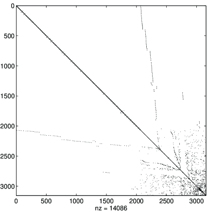
Figure 1: Sparse Pattern of the Test Matrix

The same pencil has been used in [4], where the authors report results of a parallelization of the lopsided simultaneous iteration algorithm [22]. Their strategy to find unstable modes is to perform shift-invert subspace iterations with initial shifts given on the imaginary axis. We implemented here a sequential version of this algorithm. As initial vectors we took $Z^{(0)}=LZ^{(0)}=\pmatrix{X^{(0)}\cr 0}$, where $X^{(0)}$ is a matrix with (up to) eight first column vectors of the $790\times 790$ Fourier matrix $F(j,k)=e^{j.k.\frac{2\pi i}{790}}$. After each four shift-invert iterations followed by a normalization of the vectors a Rayleigh-Ritz acceleration was done. That is, we first calculated a spectral decomposition of $B=G^{-1}H$ ([13], [20]), where $G=(LZ^{(4k)})^{H}(LZ^{(4k)})$ and $H=(LZ^{(4k)})^{H}W$, with $W=L\,(J-aL)^{-1}L\,Z^{(4k)}$, such that the Ritz values were ordered according to decreasing absolute values. Then $W$ was multiplied by the matrix of Ritz vectors and the resulting column vectors, after normalization, undertook another cycle of four iterations. Convergence was achieved when the $\infty-norm$ of the difference between corresponding vectors of $LZ^{(4k)}$ and $LZ^{(4k+1)}$ was less than a tolerance, taken to be $10^{-5}$. A deflation technique was also implemented for these tests: aside from the choice of initial vectors and the deflation technique, this is the algorithm used in [4]. Some results obtained with these iterations on SUN SPARC workstations are displayed in Table 1, where iter and prod mean respectively the number of Rayleigh-Ritz accelerations and the number of matrix-vector multiplications being performed. Notice that matrix-vector multiplication consists of backward and forward substitutions after computing an ${\cal LU}$ decomposition of $(J-aL)$, which is done only once for each $a$.

converged value	iter	prod
-0.1164+3.2018i	3	96
-0.0925+3.9827i	6	180
-0.9573+2.1594i	8	228
-0.4803+1.7632i	8	228

converged value	iter	prod
-0.0925+3.9827i	2	64
-0.1164+3.2018i	7	204
0.1814+4.8323i	7	204
-0.5911+4.6935i	8	224

Table 1: Simultaneous shift-invert method: $a=0+3i$ and $a=0+4i$

ARNCHEB performs an incomplete Arnoldi method combined with an acceleration technique using Chebyshev polynomials [2], [3]. We have used its Reverse Communication interface to calculate matrix-vector multiplications by $C_{\sigma}=I+2\,Re\,\sigma\,L\,(J-\sigma L)^{-1}$. As seen before, since $L=\pmatrix{I&0\cr 0&0}$, we avoid the spurious eigenvalue 1 with this Cayley transform by considering only the first 790 coordinates of the vectors, that is, by solving systems $(J-\sigma L)w=Lz$ and taking only the first 790 coordinates of $w$. In the tests, the dimension of the Krylov space was taken to be 54 and the number of requested eigenvalues, 4. Some results are in Table 2, where ${\cal O(r)}$ is the order of the residual $||(C_{\sigma}-\lambda I)v||_{2}$, with $||v||_{2}=1$, and iter is the number of Arnoldi steps.

converged value	${\cal O(r)}$
0.1814+4.8323i	$10^{-10}$
0.1814-4.8323i	$10^{-10}$
0.0233+0.0000i	$10^{-08}$
0.0004+0.0000i	$10^{-07}$
iter	prod
12	856

converged value	${\cal O(r)}$
0.1814+4.8323i	$10^{-11}$
0.1814-4.8323i	$10^{-11}$
0.0233+0.0000i	$10^{-08}$
0.0004+0.0000i	$10^{-08}$
iter	prod
31	2107

Table 2: ARNCHEB: $\sigma=4.0$ and $\sigma=6.0$

The same sort of experiment was carried out with ARPACK. The program dndrv1.f was rewritten to include the same routines which solved the systems in the tests with ARNCHEB. Here the dimension of the Krylov space was taken to be 20 and also 4 eigenvalues were requested to converge. Some of the results are shown in Table 3.

converged value	${\cal O(r)}$
0.1814+4.8323i	$10^{-13}$
0.1814-4.8323i	$10^{-13}$
0.0233+0.0000i	$10^{-14}$
0.0004+0.0000i	$10^{-13}$
iter	prod
301	3349

converged value	${\cal O(r)}$
0.1814+4.8323i	$10^{-14}$
0.1814-4.8323i	$10^{-14}$
0.0233+0.0000i	$10^{-14}$
0.0004+0.0000i	$10^{-13}$
iter	prod
301	3679

Table 3: ARPACK: $\sigma=4.0$ and $\sigma=6.0$

The advantage of these methods is that they require only one factorization of the pencil in upper and lower triangular factors. The disadvantage is the presence of parameters which need to be adjusted, like the dimension of the Krylov space and the convergence criterion. ARNCHEB worked well when this dimension was large compared to the number of desired eigenvalues (ten times, e.g.). The tolerance used was 1.0d-11. The opposite ocurred with ARPACK: it worked well when the dimension of the Krylov space was between four and six times the number of desired eigenvalues. The tolerance employed was 0.d0: when it was changed to 1.0d-16, the convergence for the two positive real eigenvalues was not achieved.

converged value	iter	${\cal O(r)}$
0.0004+0.0000i	6 (2)	$10^{-10}$
-0.6223+0.9649i	11 (3)	$10^{-10}$
-0.4803+1.7632i	8 (2)	$10^{-07}$
-0.0925+3.9827i	6 (2)	$10^{-11}$
-0.1351+6.8974i	8 (2)	$10^{-07}$
-1.5684+12.593i	7 (2)	$10^{-08}$

converged value	iter	${\cal O(r)}$
0.0004+0.0000i	6 (2)	$10^{-10}$
0.0233+0.0000i	10 (3)	$10^{-11}$
0.1814+4.8323i	10 (3)	$10^{-08}$
-0.0925+3.9827i	6 (2)	$10^{-09}$
-0.1351+6.8974i	9 (3)	$10^{-11}$
-0.1144+10.617i	8 (2)	$10^{-06}$

Table 4: Algorithm I - $\sigma=4.0$: $p=0$ and $p=40$

The experiments with algorithms I and II were carried out by taking only the first four column vectors of the Fourier matrix of order 790 as initial vectors. We chose initial shifts on the upper half of the unit circle, $\mu_{k}=\displaystyle{e^{\frac{k\pi i}{6}}},\;0\leq k<6$ ($k=6$ yields ($C_{\sigma}^{-1}-I$), which is singular). For each initial shift, the process stops when, for some $k$, $|x_{k}^{(j)}-x_{k}^{(j-1)}|<tol$. The tolerance $tol$ was taken as $10^{-4}$. The number $t$ of iterations performed before shift update was 4. The following tables contain the results of these tests performed in SUN SPARC workstations. The first column indicates the eigenvalue reached by the iteration. Also, iter is the number of shift-invert iterations, the number of ${\cal LU}$ factorizations appears between parenthesis, and ${\cal O(r)}$ is the order of the residual

$$||(C_{\sigma}^{-1}-\mu\,I)x||_{2},\quad||x||_{2}=1.$$

Preconditioning is performed by multiplying initial vectors $p$ times by $C_{\sigma}$, followed by normalization: $p=0$ means no preconditioning. If $p\neq 0$, multiplication by $C_{\sigma}$ requires an additional ${\cal LU}$ decomposition. In order to know how many matrix-vector multiplications were performed in the tests, multiply iter by 4 and add $4p$.

$\lambda$	iter	${\cal O(r)}$
0.0004+0.0000i	6 (2)	$10^{-10}$
-0.4803+1.7632i	7 (2)	$10^{-07}$
-0.1164+3.2018i	8 (2)	$10^{-07}$
-0.1764+6.1231i	7 (2)	$10^{-08}$
-0.1144+10.617i	5 (2)	$10^{-10}$
-1.5684+12.593i	11 (3)	$10^{-09}$

converged value	iter	${\cal O(r)}$
0.0004+0.0000i	6 (2)	$10^{-10}$
0.0233+0.0000i	10 (3)	$10^{-08}$
0.1814+4.8323i	10 (3)	$10^{-08}$
-0.1764+6.1231i	8 (2)	$10^{-07}$
-0.1144+10.617i	4 (1)	$10^{-06}$
-101.95+0.0000i	18 (5)	$10^{-09}$

Table 5: Algorithm I - $\sigma=6.0$: $p=0$ and $p=40$

For the algorithm II, $\sigma$ was chosen to be 4.8334, the modulus of the unstable eigenvalues $0.1814\pm 4.8323i$. From the previous section, this is the real value for $\sigma$ that maximizes the absolute value of the corresponding eigenvalues of the Cayley transform $C_{\sigma}$. Thus, preconditioning of the initial vectors with this $\sigma$ should make these eigenvalues easier to detect. Indeed, in Table 6 we can see that one of them was identified from two consecutive initial shifts. In the same table are listed the results when the procedure of inhibiting the last found eigenvalue was applied (for the first initial shift, there is nothing to inhibit). In Table 7 a better performance of the inhibiting procedure can be seen: the convergence to the two unstable eigenvalues was achieved.

The ${\cal LU}$ decomposition of $(J-aL)$ is about 150 times slower than the resolution of the corresponding systems on a SUN SPARC 4 workstation (typical runtimes were 7.05078 and 4.29688e-02, respectively). Thus, Algorithms I and II had a performance comparable to the others in respect to time and accuracy. For instance, from Table 4, we see that by preconditioning the vectors we obtained three unstable modes and three stable ones (two of these are low damped), after 196+160 matrix-vector multiplications (indeed, backward and forward substitutions) and 15+1 factorizations.

$\lambda$	iter	${\cal O(r)}$
0.0004+0.0000i	6 (2)	$10^{-10}$
0.0233+0.0000i	10 (3)	$10^{-09}$
0.1814+4.8323i	12 (3)	$10^{-06}$
0.1814+4.8323i	6 (2)	$10^{-08}$
-0.1144+10.617i	9 (3)	$10^{-12}$
-200.38+0.0000i	15(4)	$10^{-09}$

converged value	iter	${\cal O(r)}$
0.0004+0.0000i	6 (2)	$10^{-10}$
-0.1764+6.1231i	12(3)	$10^{-07}$
0.0233+0.0000i	10 (3)	$10^{-09}$
0.1814+4.8323i	6 (2)	$10^{-07}$
-0.1144+10.617i	8 (2)	$10^{-08}$
-200.38+0.0000i	11(3)	$10^{-12}$

Table 6: Algorithm I and II - $\sigma=4.8334$, $p=40$

$\lambda$	iter	${\cal O(r)}$
0.0004+0.0000i	6 (2)	$10^{-10}$
0.0233+0.0000i	8 (2)	$10^{-06}$
0.1814+4.8323i	7 (2)	$10^{-06}$
0.1814+4.8323i	6 (2)	$10^{-10}$
-0.1144+10.617i	13(4)	$10^{-12}$
-0.1144+10.617i	8(2)	$10^{-07}$

converged value	iter	${\cal O(r)}$
0.0004+0.0000i	6 (3)	$10^{-10}$
0.1814+4.8323i	13 (5)	$10^{-09}$
0.1814-4.8323i	9 (4)	$10^{-08}$
0.1814+4.8323i	6 (3)	$10^{-09}$
-0.1144+10.617i	7 (3)	$10^{-07}$
0.1814-4.8323i	10 (4)	$10^{-07}$

Table 7: Algorithm I and II - $\sigma=4.8334$, $p=80$

References

- [1] L. H. Bezerra, Stability Analysis of Large Scale Power Systems (in Portuguese), D. Thesis, Pontifícia Universidade Católica, Rio de Janeiro, 1990.
- [2] T. Braconnier, ’The Arnoldi Chebyshev Algorithm for Solving Large Nonsymmetric Eigenproblems’, Technical Rep. TR/PA/93/25, CERFACS, Toulouse.
- [3] T. Braconnier, V. Fraysse and J.-C. Rioual, ’ARNCHEB Users’ Guide: Solution of Large Nonsymmetric or Non Hermitian Eigenvalue Problems by the Arnoldi-Chebyshev Method’, Technical Rep. TR/PA/97, CERFACS, Toulouse.
- [4] J. M. Campagnolo, N. Martins, J. L. R. Pereira, L. T. G. Lima, H. J. C. P. Pinto, and D. M. Falcão, ’Fast Small-Signal Stability Assessment Using Parallel Processing’, IEEE Trans. on Power Systems, PWRS-9(2), 949-956, 1994.
- [5] F. Chatelin and D. Ho, ’Arnoldi-Chebyshev Procedure for Large Scale Nonsymmetric Matrices’, Math. Model. Numer. Anal., 24, 53-65, 1990.
- [6] K. A. Cliffe, T. J. Garratt and A. Spence, ’Eigenvalues of the Discretized Navier-Stokes Equation with Application to the Detection of Hopf Bifurcations’, Advances in Computational Mathematics, 1(2), 337-356, 1993.
- [7] K. A. Cliffe, T. J. Garratt and A. Spence, ’Eigenvalues of Block Matrices Arising from Problems in Fluid Mechanics’, SIAM J. Matrix Anal. Appl., 15(4), 1310-1318, 1994.
- [8] I. S. Duff and J. A. Scott, ’Computing Selected Eigenvalues of Sparse Unsymmetric Matrices Using Subspace Iteration’, ACM Trans. Math. Softw., 19(2), 137-159, 1993.
- [9] G. H. Golub and C. F. Van Loan, Matrix Computations, 2nd ed., The Johns Hopkins University Press, Baltimore, 1989.
- [10] A. Jennings and J. J. McKeowen, Matrix Computations, 2nd ed., John Wiley and Sons, New York, 1992.
- [11] A. Jennings and W. J. Stewart, ’Simultaneous Iteration for Partial Eigensolution of Real Matrices’, J. Inst. Maths. Applics., 15, 351-361, 1975.
- [12] P. Kundur, Power System Stability and Control, McGraw Hill, New York, 1994.
- [13] E. Anderson, Z. Bai, C. Bischof, J. Demmel, J. Dongarra, J. DuCroz, A. Greenbaum, S. Hammarling, A. McKenney, S. Ostrouchov, and D. Sorensen, LAPACK Users’ Guide, Release 2.0, 2nd ed., SIAM Publications, Philadelphia, 1995.
- [14] R. B. Lehoucq, D. C. Sorensen and C. Yang, ’ARPACK Users’ Guide: Solution of Large Scale Eigenvalue Problems by Implicitly Restarted Arnoldi Methods’, July 1996.
- [15] L. T. G. Lima, L. H. Bezerra, C. Tomei and N. Martins, ’New Methods for Fast Small Signal Stability Assessment of Large Scale Power Systems’, IEEE Transactions on Power Systems, 10(4), 1979-1985, November 1995.
- [16] N. Martins, ’Efficient Eigenvalue and Frequency Response Methods Applied to Power System Small-Signal Stability Studies’, IEEE Trans. on Power Systems, PWRS-1(1), 217-226, February 1986.
- [17] K. Meerbergen and D. Roose, ’Matrix Transformations for Computing Rightmost Eigenvalues of Large Sparse Non-Symmetric Eigenvalue Problems’, IMA J. Numer. Anal., 16, 297-346, 1996.
- [18] Y. Saad, ’Chebyshev Acceleration Techniques for Solving Nonsymmetric Eigenvalue Problems’, Math. Comp., 42, 567-588, 1984.
- [19] J. A. Scott, ’An Arnoldi Code for Computing Selected Eigenvalues of Sparse Real Unsymmetric Matrices’, ACM Trans. Math. Softw., 21(4), 432-475, 1995.
- [20] B. T. Smith et al., Matrix Eigensystem Routines: EISPACK Guide, 2nd ed., Springer Verlag, New York, 1976.
- [21] D. C. Sorensen, ’Implicit Application of Polynomial Filters in a K-Step Arnoldi Method’, SIAM J. Matrix Anal. Appl., 13(1), 357-385, 1992.
- [22] W. J. Stewart and A. Jennings, ’A Simultaneous Iteration Algorithm for Real Matrices’, ACM Trans. Math. Softw., 7(2), 184-198, 1981.
- [23] N. Uchida and T. Nagao, ’A New Eigen-Analysis Method of Steady-State Stability Studies for Large Power Systems: S-Matrix Method’, IEEE Trans. on Power Systems, PWRS-3(2), 706-714, May 1988.
- [24] L. Wang and A. Semlyen, ’Application of Sparse Eigenvalue Techniques to the Small-Signal Stability Analysis of Large Power Systems’, IEEE Trans. on Power Systems, PWRS-5(2), 635-642, May 1990.
- [25] D. S. Watkins, Fundamentals of Matrix Computations, John Wiley and Sons, New York, 1991.