Nonautonomous Food-Limited Fishery Model With Adaptive Harvesting

Abstract

We will introduce the biological motivation of the $\gamma$- food-limited model with variable parameters. New criteria are established for the existence and global stability of positive periodic solutions. To prove the existence of steady-state solutions, we used the upper-lower solution method where the existence of at least one positive periodic solution is obtained by constructing a pair of upper and lower solutions and application of the Friedreichs Theorem. Numerical simulations illustrate effects of periodic variation in the values of the basic biological and environmental parameters and how the adaptive harvesting strategies affect fishing stocks.

Keywords-Fishery models, Nonautonomous Differential Equations, Harvesting Strategies, Food-Limited Model, Adaptive Harvesting, Periodic Solutions, Stability.
Math Subject Classifications: 34C25, 34D23, 92B05

I Time-Varying Fishery Models: Biological motivation

Most populations experience regular or recurring fluctuations in biological and environmental factors which affect demographic parameters [1]–[3], [8], [10], [11], [15], and mathematical models cannot ignore for example, year-to-year changes in weather, the global climate variability, habitat destruction and exploitation, the expanding food surplus, and other factors that affect the population growth [1]–[5], [11], [16], [20]–[24] and [27]. In most models of population dynamics, increases in population due to birth are assumed to be time-independent, but many species reproduce only during a single period of the year. There are several biological parameters that can vary seasonally, including some cyclical changes in control parameters. For example, in temperature or polar zones growth frequently slows down, or even ceases in winter. Careful analysis in [21] shows that there might be a relationship between asymptotic recruitment and bottom temperature, i.e., stocks located in warmer waters had lower asymptotic recruitment.

Consider the following autonomous model for the harvested population with size $N(t)$ at time $t$ :

$$\frac{1}{N}\frac{dN}{dt}=G(N)-E$$ (1)

where

$$G(0)=r\,,\qquad G(K)=0.$$

We assume that $G(N)$ is strictly decreasing, and define the intrinsic growth rate $r>0$ for $N\approx 0$, the carrying capacity $K>0$, and the effort function $E$.
The linearity assumption in the logistic model is violated for nearly all populations, e.g. for a food-limited population Smith [25] (see [26]) reported a snag in the classical logistic model, i.e. it did not fit experimental data, and suggested a modification of the logistic equation

$$\frac{1}{N}\frac{dN}{dt}=G(N|r,K,\beta)-E,$$ (2)

where $G(N|r,K,\beta)=r(1-N/K)(1+\beta N/K)^{-1}$, and Smith [25] called the coefficient $(1+\beta N/K)^{-1}$ the delaying factor.
Let $x(t)=\frac{N(t)}{K}$, then equation (2) has the form

$$\frac{dx}{dt}=rx\frac{1-x}{1+\beta x}-Ex$$

To take into consideration a crowding factor , we introduce a new function

$$G(x|r,\beta,\gamma)=r(1-x^{\gamma})(1+\beta x^{\gamma})^{-1},$$ (3)

where $\gamma>0$. Then equation (1) takes a form

$$\frac{dx}{dt}=rx\frac{1-x^{\gamma}}{1+\beta x^{\gamma}}-Ex.$$

It is clear, if $\beta=0$, the function $G(x)$ in (3) is concave and $G(x)\rightarrow-\infty$ as $x\rightarrow\infty$. If $\beta>0$, then $G(x)$ is sigmoidal with $-\frac{r}{\beta}<G(x)\leq r$.

Remark. Let $G_{1}(x)=x(1-x^{\gamma})(1+\beta x^{\gamma})^{-1}$. Clearly (see for example Fig 1 below) function $G_{1}(x)$ has a unique maximum on the interval $x\in(0,1)$,

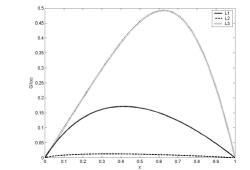
Figure 1: Different forms of function $G_{1}(x)$ (L1: $\beta=0,\gamma=1$; L2: $\beta=0.2,\gamma=5$; L3: $\beta=4,\gamma=0.5$)

and the maximum value and the position of a critical point depend on some combinations of the parameters $\gamma$ and $\beta$. If $\beta=0$ and $\gamma=1$ then $G_{1}(x)$ is a classical symmetrical logistic function.
We construct a time-varying (nonautonomous) model based on equation (2) by allowing $r(t)$ and $K(t)$ to vary, while maintaining constant parameters $(\beta,\gamma)$. Similar model for unharvested population was studied in [11] under the assumption that $K$ and $r$ oscillate with small amplitudes. For an exploited marine population we introduce a varying effort function $E=E(t)$.

$$\frac{1}{N}\frac{dN}{dt}=r(t)\left[1-\left(\frac{N}{K(t)}\right)^{\gamma}\right]\left[1+\beta\left(\frac{N}{K(t)}\right)^{\gamma}\right]^{-1}-E(t),$$ (4)

where $N|_{t=0}=N_{0}>0.$
In population dynamics the term $\left(\frac{N}{K}\right)^{\gamma}$ is refereed to as the Richards’ nonlinearity [26].
Denote

$$\overline{N}=\int_{0}^{T}N(s)ds$$

and

$$\overline{K}=\int_{0}^{T}K(s)ds,$$

where $T>0$ is the period of the system. Illustrative periodic functions $K(t)$ and $r(t)$ can be of the forms:

$$r(t)=r_{0}\left[1+\alpha_{r}\sin\frac{2\pi(t-\phi_{r})}{T_{r}}\right]$$ (5)

$$K(t)=K_{0}\left[1+\alpha_{K}\sin\frac{2\pi(t-\phi_{K})}{T_{K}}\right]$$ (6)

Parameters $r_{0}$, $K_{0}$, $\alpha$, and $T$ can be different for $r$ and $K$. We assume, however, that periods have a lowest common multiple, which defines the period for the system.
For a canonical logistic equation it was proven that $\overline{N}$ decreased as the magnitude of variation in $K$ increases, and that $\overline{N}\leq\overline{K}$ irrespective to $r$. However, it was shown in [11] that the effect of the environmental cycles is ”a very model-dependent phenomenon”.

Harvesting population models with a periodic function $E(t)$ have been studied extensively in recent years [5]–[9], [13], [17]– [20]. However, function $E(t)$ is not a periodic function, in fact, it is a function of many (continuous) variables which fishery managers can manipulate and this function can be defined by the fishery strategies. For example, adaptive harvesting strategies in fisheries [12] rests on a combination of three elements: (a) deduction from prior knowledge of the ecosystem’s components, (b) experience with similar ecosystems elsewhere, coupled with (c) mathematical modeling. Adaptive fishery strategies fit better with new multi-species management, with more emphasis on an ”ecosystem approach” to sustainable fishery management. The study of the dynamical behaviors of the Fox harvesting models

$$\frac{1}{N}\frac{dN}{dt}=r(t)\ln^{\gamma}\frac{K(t)}{N}-E(t).$$ (7)

in periodical environments were introduced in [5] and [17].

The paper is organized as follows. In the next section we study qualitative behavior of the solutions of a harvesting model in constant environments and obtain the explicit conditions for the existence of a unique positive solution of equation. In Section 3 for equation (4) we will prove that it possess positive, bounded, asymptotically stable periodic solutions. In Section 4 we will investigate numerically the effects of periodic variation in the values of the basic population parameters $r(t)$ and $K(t)$ and discuss adaptive vs static harvesting strategies.

II Autonomous Model with Proportional Harvesting

Consider equation (I) with proportional harvesting

$$\frac{dx}{dt}=rx[1-x^{\gamma}][1+\beta x^{\gamma}]^{-1}-Ex.$$ (8)

If $\beta=0$ then (8) is an alternative to the logistic fishing model with the Richards’ nonlinearity

$$\frac{dx}{dt}=rx(1-x^{\gamma})-Ex.$$ (9)

Equation (8) has a nontrivial equilibrium point

$$x_{Ge}=\sqrt[\gamma]{\frac{1-E^{*}}{1+\beta E^{*}}},$$

and equation (9) has a nonzero equilibrium point

$$x_{Le}=\sqrt[\gamma]{1-E^{*}},$$

where $E^{*}=E/r$ and $0<E<r$.

For the corresponding annual equilibrium harvests $Y_{Ge}(E)=Ex_{Ge}$ and $Y_{Le}(E)=Ex_{Le}$,
$x_{Ge}<x_{Le}$ and $Y_{Ge}\ <Y_{Le}$. Note that the maximum sustainable yield ($\max_{E}Y(E)$) exists for $E\in(0,r/q)$.

Let $u=\ln x$ then equations (8) has the following form

$$\frac{du}{dt}=\Phi(u)-E,$$

where

$$\Phi(u)=r\frac{1-e^{u\gamma}}{1+\beta e^{u\gamma}}.$$

Note

$$\frac{d\Phi}{du}=\Phi^{\prime}(u)=-\gamma re^{\gamma u}\frac{1+\beta}{\left(1+\beta e^{\gamma u}\right)^{2}}<0$$

and positive equilibrium

$$x^{*}=\sqrt[\gamma]{\frac{1-E^{*}}{1+\beta E^{*}}}$$

of (8) is locally asymptotically stable.

      Theorem II.1.

If in equation (8) we assume that $r,K,\beta,E$ and $\gamma$ are all positive constants, then

$a1)$ If $r>E$ then for every solution $x(t)$

$$\lim_{t\rightarrow\infty}x(t)=x^{*}$$

exists.

$a2)$ If $E\equiv 0$ then $\lim_{t\rightarrow\infty}x(t)=1.$

Proof. The solution to equation (8) has an implicit form

$$E^{*}-1+(\beta E^{*}+1)x^{\gamma}=Cx^{\alpha\gamma}\exp(-r\alpha\gamma(1-E^{*})t)\$$

with

$$\alpha=\frac{1+E^{*}\beta}{1+\beta},$$

$C$ is an arbitrary constant. As $t\rightarrow\infty$

$$x(t)\rightarrow\sqrt[\gamma]{\frac{1-E^{*}}{1+E^{*}\beta}}=x^{*}\text{ }.$$

To prove the second part of the theorem, we note that if $E\equiv 0$ then the solution of (8) takes a form

$$-1+x^{\gamma}=Cx^{\alpha\gamma}\exp(-\gamma\alpha rt)\$$

thus

$$\lim_{t\rightarrow\infty}x(t)=1.$$

III Nonautonomous Model with Seasonal Harvesting

Let us assume that all parameters in (4) are continuous functions and for all $t\geq 0$

$$\frac{1}{N}\frac{dN}{dt}=r(t)\frac{K^{\gamma}(t)-N^{\gamma}}{K^{\gamma}(t)+\beta N^{\gamma}}-E(t),$$ (10)

where $\gamma>0$ and $\beta>0.$

      Definition III.1.

We say that a positive solution $N^{\ast}(t)$ of equation (10) is a global attractor or globally asymptotically stable (GAS) if for any positive solution $N(t)$

$$\lim_{t\rightarrow\infty}|N(t)-N^{\ast}(t)|=0.$$

Usually $N^{\ast}(t)$ is a positive equilibrium or a positive periodic solution of equation (10) if it exists. In general, we will use the following definition.

      Definition III.2.

We say that equation (10) is GAS, if for every two positive solutions $N_{1}(t)$ and $N_{2}(t)$ of equation (10) we have

$$\lim_{t\rightarrow\infty}|N_{1}(t)-N_{2}(t)|=0.$$

Note that canonical logistic equation with variable parameters has been well-studied, and the questions of the existence and stability in this case are easily handled since the equation is solvable as a Riccati equation in a closed form [1]–[3], [10], [20] and [23].

      Theorem III.1.

Assume that

$$E_{1}(t)=E(t)+\frac{1}{K}\frac{dK}{dt}>0$$ (11)

and $r(t),K(t)$ and $E(t)$ are positive functions. If $0<N(0)<K(0)$, then every solution of equation (10) satisfies the following inequality $0<N(t)<K(t)$ for all $t\geq 0.$

Proof. Let $v(t)=\ln\frac{N(t)}{K(t)},$ then equation (11) has a form

$$\frac{dv}{dt}=r(t)\frac{1-e^{v\gamma}}{1+\beta e^{v\gamma}}-E_{1}(t),$$ (12)

where $v(0)<0.$ Let us prove that $v(t)<0$ for all $t\geq 0.$ Suppose there exists $t_{1}>0$ such that $v(t_{1})=0.$ Then

$$\frac{dv}{dt}\mid_{t_{1}}=-E_{1}(t_{1})<0.$$

Therefore in some interval ($t_{1}-a,t_{1})$ the function $v(t)$ is decreasing and $v(t_{1})=0.$ But this is impossible, therefore $v(t)<0$ follows by $N(t)<K(t).$
To prove our next theorems for the periodic models we will use [14] (see also [5]).

      Theorem III.2.

(Friedrichs Theorem). Suppose that $G(t,N)$ is a smooth function with period $T$ in $t$ for every $N$. Suppose also that there exist constants $a,b$ with $a<b$ such that $G(t,b)<0<G(t,a)$ for every $t$. Then there is a periodic solution $N_{0}(t)$ of the differential equation $dN/dt=G(t,N)$ with period $T$ and $N(0)=c$ for some $c\in(a,b).$

      Theorem III.3.

Consider equation (4). For all $\gamma>0,\beta\geq 0$ and $t\geq 0$ we assume that $E(t),r(t),K(t)$ are all positive $T-$periodic functions, and $r(t)-E_{1}(t)>0$ for all $t\geq 0.$ Then there exists a positive nonconstant periodic solution $N_{0}(t)$ such that

$$K(0)e^{b_{0}}<N_{0}(0)<K(0),$$

where

$$b_{0}<\frac{1}{\gamma}\min\lim_{t\in[0,T]}\ln\frac{r(t)-E_{1}(t)}{r(t)+\beta E_{1}(t)}<0.$$

Proof. Let $v=\ln\frac{N(t)}{K(t)},$ then equation (4) has a form

$$\frac{dv}{dt}=r(t)\frac{1-e^{v\gamma}}{1+\beta e^{v\gamma}}-E_{1}(t)=\Phi(t,v).$$ (13)

Clearly, $\Phi(t,0)=-E_{1}(t)$ $<0$ and

$$\Phi(t,b_{0})=r(t)\frac{1-e^{b_{0}\gamma}}{1+\beta e^{b_{0}\gamma}}-E_{1}(t)\ >0.$$

The last inequality is equivalent to the inequality

$$\text{\ }\frac{1}{\gamma}\ln\frac{r(t)-E_{1}(t)}{r(t)+\beta E_{1}(t)}>b_{0}.$$

Therefore based on Theorem (III.2), there exists periodic solution $v_{0}(t)$ of equation (13), such that $b_{0}<v_{0}(t)<0.$ That yields the existence of the periodic solution $N_{0}(t)$ of equation (4) such that

$$K(0)e^{b_{0}}<N_{0}(0)<K(0).\text{\ }$$

      Theorem III.4.

Suppose all conditions of Theorem (III.3) hold. Then there exists a unique periodic solution $N_{0}(t)>0$ of equation (4) such that $0<N_{0}(0)<K(0)$  and

$$\lim_{t\rightarrow\infty}[N(t)-N_{0}(t)]=0.$$

Proof. According to Theorem (III.1) the solution $v(t)$ of equation (12) is negative for all $t\geq 0.$ Firstly, let us prove that

$$\lim_{t\rightarrow\infty}\inf v(t)>-\infty.$$ (14)

Assume that

$$\lim_{t\rightarrow\infty}v(t)=-\infty.$$

Then

$$\lim_{t\rightarrow\infty}\inf\frac{dv}{dt}=\lim_{t\rightarrow\infty}\inf[r(t)-E_{1}(t)]>0,$$

and

$$\lim_{t\rightarrow\infty}v(t)=\lim_{t\rightarrow\infty}\left[v(0)+\int_{0}^{t}\frac{dv}{ds}\right]=\infty.$$

We have a contradiction. If $\lim_{t\rightarrow\infty}v(t)$ does not exist, then there exists a sequence $\{t_{n}\}$ such that $v(t_{n})\rightarrow-\infty$ and

$$\frac{dv}{dt}|_{t_{n}}=0.$$ (15)

Then equality (17) yields

$$r(t_{n})-E_{1}(t_{n})\rightarrow 0.$$

That contradiction proves statement (14). Suppose $N_{1}(t)$ and $N_{2}(t)$ are two positive solutions of equation (12) with $0<N_{i}(t)<K(0)$ $i=1,2$. Then

$$v_{1}(t)=\ln\frac{N_{1}(t)}{K(t)}$$

and

$$v_{2}(t)=\ln\frac{N_{2}(t)}{K(t)}$$

are two solutions of equation (12). Assume that $v_{1}(t)<v_{2}(t).$ Let

$$v(t)=v_{2}(t)-v_{1}(t).$$

Then equation (12) takes the form

$$\frac{dv}{dt}=r(t)\left[\frac{1-e^{v_{2}\gamma}}{1+\beta e^{v_{2}\gamma}}-\frac{1-e^{v_{1}\gamma}}{1+\beta e^{v_{1}\gamma}}\right].$$ (16)

Application of the Mean-Value Theorem transforms equation (16) to

$$\frac{dv}{dt}=-a(t)v(t)$$ (17)

with

$$a(t)=r(t)\left\{\frac{(1+\beta)\gamma e^{c(t)\gamma}}{[1+\beta e^{c(t)\gamma}]^{2}}\right\},$$

where

$$\int_{0}^{\infty}a(s)ds=\infty$$

and

$$v_{1}(t)<c(t)<v_{2}(t).$$

Based on the last inequality

$$\liminf_{t\rightarrow\infty}v(t)>-\infty,$$

$$\liminf_{t\rightarrow\infty}c(t)>-\infty.$$

Hence $\liminf_{t\rightarrow\infty}a(t)>0,$ therefore for every solution of (17) we have $\lim_{t\rightarrow\infty}v(t)=0,$ or $\lim_{t\rightarrow\infty}[v_{1}(t)-v_{2}(t)]=0.$ Similarly, if $v_{1}(t)>v_{2}(t)$, then $\lim_{t\rightarrow\infty}[v_{2}(t)-v_{1}(t)]=0.$ Summing up, we conclude $\lim_{t\rightarrow\infty}[N_{1}(t)-N_{2}(t)]=0.$

Remark. If $N_{1}(t)$ and $N_{2}(t)$ are any two solutions of equation (4), then statement of Theorem 3.4 is true without the assumption that all functions $r(t)$, $K(t)$ and $E(t)$ are $T$-periodic.

IV Numerical Experiments

Fig 2 illustrates dynamics of the population for a different set of parameters $\alpha$ and $\beta$.

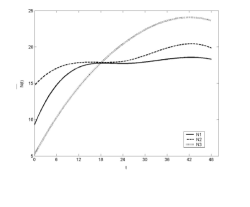
Figure 2: Size of the population for different models: N1: $\beta=0,\gamma=1$ logistic; N2: $\beta=0.2,\gamma=5$; N3: $\beta=4,\gamma=0.5$

Fig 3 supports a well-known feature of the population models: increase in the amplitude of the carrying capacity $K(t)$, defined by equation (6), yields decrease in the average size of the population, whereas,

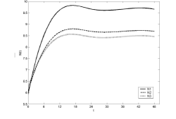
Figure 3: Change of environment. Population size for different values of $\alpha_{K}$ (N1: $\alpha_{K}=0.1$, N2: $\alpha_{K}=0.5$ and N3: $\alpha_{K}=0.7$).

Fig 4 proves that the qualitative behavior of the system is unchanged [23] by oscillations in $r(t)$, defined by equation (5), alone.
Remark. In all numerical experiments below we used parameters $E(t)$ and $K(t)$ that satisfy the condition (11).

The qualitative behavior of the system depends critically on the phase difference of the oscillations in $r(t)$ and $K(t)$. For example, if functions $r(t)$ and $K(t)$ have a $180^{\circ}$ phase shift, then the relationship between the average population size and environmental and demographic variations (see Fig 5) is very different from the corresponding Fig 3.

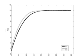
Figure 4: Change of demography. Population size for different values of $\alpha_{r}$ (N1: $\alpha_{r}=0.1$, N2: $\alpha_{r}=0.5$ and N3: $\alpha_{r}=0.9$).

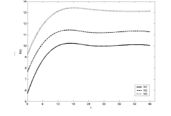
Figure 5: Change of phase shift. Population size for different values of $\alpha_{K}$ (N1: $\alpha_{K}=0.1$, N2: $\alpha_{K}=0.5$ and N3: $\alpha_{K}=0.7$).

Often debated questions are the choice of the harvesting strategies and timing of harvesting. For simplicity, we consider static vs adaptive fishing strategies.

Static Fishing Strategy. Consider a fishery manager who has no access to previous fishery data. He starts fishing (on Fig 6 curve $N1$) all year with an annual quota of 12 tons and realized that in one-year period a fishstock is decreased significantly. Then the manager decides to shorten a fishing season, starts it in June and fishes for six months with a monthly quota of 2 tons (curve $N2$), and thereafter, he starts in September with the quota of 4 tons per month and fishes three months ( curve $N3$ ),

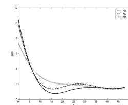
Figure 6: Static Fishing Strategy

Adaptive Fishing Strategy. Let a fishery manager have access (Fig 7 first graph) to the fishery data. He decides to fish in March because at that time the population attains its maximum. Curve $N2$ represents a six-month fishing, starting in March with 2 tons per month, whereas on curve $N3$, fishing takes place with the quota of 4 tons per month but in a three-month period. Clearly, the latter strategy is more efficient than the static strategy (curve $N1$ on Fig 7) which represents a greater risk of depletion of the fishstock.

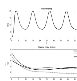
Figure 7: Adaptive Fishing Strategy

V Discussion

In this paper we illustrate various effects of the varying environmental carrying capacity and intrinsic rates on dynamics of marine populations. Application of the food-limited model with $\gamma$-nonlinearity is consistent with fishery data, and supports a well-known feature of the population models: average population size decreases with an increase of amplitude of variation in the carrying capacity $K(t)$, but $\overline{N}\leq\overline{K}$ and the dynamics of the population must ride on this highly variable resource. On other hand, even large oscillations in $r(t)$ alone leave the system’s behavior practically unchanged. Note that similar results were obtained for the Fox fishery model (7) in [17]. However, the qualitative behavior of the system depends critically on the phase difference between the oscillations in $r(t)$ and $K(t)$. For example, if functions $r(t)$ and $K(t)$ have a $180^{\circ}$ phase shift then the relationship between the average population size and environmental and demographic variations is very different.
With no access to fisheries data a static fishing strategy represents a greater risk of extinction of marine populations under severe harvesting, compared with adaptive strategies that save fishstock in a cost effective manner.

Acknowledgements
We wish to express thanks to Dr. D. Barker (Fisheries and Aquaculture department at Vancouver Island University) whose comments significantly improved the text.

References

- [1] Boyce, M., Daley, D., Population Tracking of Fluctuating Environments and Natural Selection for Tracking Ability, The American Naturalist, 115 no. 4 (1980) 480-491
- [2] Boyce, M., Population Viability Analysis , Annual Review of Ecology and Systematics, 23 (1992) 481-506
- [3] Boyce, M., Sinclair, A., White, G., Seasonal Compensation of Predation and Harvesting, Oikos, 87 no. 3 (1999) 419-426
- [4] Brauer, F., Castillo-Chavez, C., Mathematical Models in Population Biology and Epidemiology, Springer-Verlag, 2001
- [5] Brauer, F., Sanchez D., Periodic environment and periodic harvesting, Natural Resource Modeling 16 (2003) 233-244
- [6] Caddy, J., Cochrane, K., A review of fisheries management past and present and some future perspectives for the third millennium Ocean and Coastal Management, 44 no. 9-10 (2001) 653-682
- [7] Chau, N., Destabilizing effect of periodic harvesting on population dynamics, Ecological Modelling, 127 (2000) 1-9
- [8] Clark, C., Mangel, M., Dynamic State Variables in Ecology: Methods and Applications. New York: Oxford University Press, 2000
- [9] Cooke, K., Nusse, H., Analysis of the complicated dynamics of some harvesting models, J. of Math. Biology, 25 (1987) 521-542
- [10] Cushing, J., Costantino, R. , Dennis, B., Desharnais, R., Nonlinear population dynamics: models, experiments and data, J. Theor. Biol. 194 (1998) 1-9
- [11] Cushing, J., Oscillatory population growth in periodic environments, Theo. Population Biology 30 no. 3 (1986) 289-308
- [12] FAO The Ecosystem Approach to Fisheries, Edited by G Bianchi, H R Skjoldal, Institute of Marine Research, Norway (2006)
- [13] Hart, D., Yield- and biomass-per-recruit analysis for rotational fisheries, with an application to the Atlantic sea scallop (Placopecten magellanicus) Fishery Bulletin, 101 no. 1 (2003) 44-57
- [14] Hartman, P., Ordinary differential equations. SIAM Classics in Applied Mathematics 38, 2002
- [15] Hseih, C., Ohman M., Biological responses to environmental forcing: the linear tracking window, Ecology, 87 no. 8 (2006) 1932-1938
- [16] Hutchings, J., Baum, J., Measuring Marine Fish Biodiversity: Temporal Changes in Abundance, Life History and Demography Philosophical Transactions: Biological Sciences, 360, no. 1454 ( 2005) 315-338
- [17] Idels, L., Stability Analysis of Periodic Fox Production Models, Canadian Applied Math. Quarterly, 14 no. 3 (2006) 333-343
- [18] Jensen, A., Harvest in a fluctuating environment and coservative harvest for the Fox surplus production model, Eco. Mod. 182 (2005) 1-9
- [19] Jerry, M., Raissi N., A policy of fisheries management based on continuous fishing effort, J. of Biological Systems, 9 (2001) 247-254
- [20] Lazer, A., Sanchez, D., Periodic Equilibria under Periodic Harvesting, Math. Magazine, 57 no. 3 (1984) 156-158
- [21] Meyer, P. , Ausubel, J., Carrying capacity: A model with logistically varying limits, Tech. Forecasting and Social Change, 61 no. 3 (1999) 209-214
- [22] Myers, R., MacKenzie, B., Bowen, K., What is the carrying capacity for fish in the ocean? A meta-analysis of population dynamics of North Atlantic cod, Can. J. Fish. Aquat. Sci. 58 (2001) 1464-1476
- [23] Nisbet, R., Gurney, W., Population Dynamics in a Periodically Varying Environment, J. of Theor. Biology 56 (1976) 459-475
- [24] Rose, K., Cowan, J., Data, models, and decisions in U.S. Marine Fisheries Management Lessons for Ecologists, Annual Review of Ecology, Evolution, and Systematics, 34 (2003) 127-151
- [25] Smith, F., Population dynamics in daphnia magna and a new model for population growth, Ecology, 44 no. 4 (1963) 651-663
- [26] Tsoularis, A., Wallace, J., Analysis of logistic growth models, Mathematical Biosciences, 179 (2002) 21-55
- [27] Vladar, H., Density-dependence as a size-independent regulatory mechanism, J. of Theor. Biology 238 (2006) 245-256