Technical Report: MIMO B-MAC Interference Network Optimization under Rate Constraints by Polite Water-filling and Duality

Abstract

We take two new approaches to design efficient algorithms for transmitter optimization under rate constraints to guarantee the Quality of Service in general MIMO interference networks, named B-MAC Networks, which is a combination of multiple interfering broadcast channels (BC) and multiaccess channels (MAC). Two related optimization problems, maximizing the minimum of weighted rates under a sum-power constraint and minimizing the sum-power under rate constraints, are considered. The first approach takes advantage of existing efficient algorithms for SINR problems by building a bridge between rate and SINR through the design of optimal mappings between them so that the problems can be converted to SINR constraint problems. The approach can be applied to other optimization problems as well. The second approach employs polite water-filling, which is the optimal network version of water-filling that we recently found. It replaces almost all generic optimization algorithms currently used for networks and reduces the complexity while demonstrating superior performance even in non-convex cases. Both centralized and distributed algorithms are designed and the performance is analyzed in addition to numeric examples.

I Introduction

I-A System Setup and Problem Statement

We study the optimization under rate constraints for general multiple-input multiple-output (MIMO) interference networks, named MIMO B-MAC networks [1], where each transmitter may send data to multiple receivers and each receiver may collect data from multiple transmitters. Consequently, the network is a combination of multiple interfering broadcast channels (BC) and multiaccess channels (MAC). It includes BC, MAC, interference channels, X channels [2, 3], X networks [4] and most practical wireless networks, such as cellular networks, WiFi networks, DSL, as special cases. We assume Gaussian input and that each interference is either completely cancelled or treated as noise. A wide range of interference cancellation is allowed, from no cancellation to any cancellation specified by a valid binary coupling matrix of the data links. For example, simple linear receivers, dirty paper coding (DPC) [5] at transmitters, and/or successive interference cancellation (SIC) at receivers may be employed.

Two optimization problems are considered for guaranteeing the Quality of Service (QoS), where each data link has a target rate. The feasibility of the target rates can be solved by a feasibility optimization problem (FOP) which maximizes the minimum of scaled rates of all links, where the scale factors are the inverse of the target rates. All target rates can be achieved simultaneously if and only if the optimum of FOP is greater than or equal to one. FOP can be used in admission control. If the target rates are feasible, the system tries to operate at minimum total transmission power in order to prolong total battery life and to reduce the total interference to other networks by solving the sum power minimization problem (SPMP) under the rate constraints.

We study both centralized and distributed optimizations. The centralized optimization with global channel state information (CSI) provides an upper bound of the performance and a stepping stone to the design of the distributed optimization algorithms. In some cases such as cooperative cellular networks, it is possible to obtain global CSI if the base stations are allowed to exchange CSI, making the centralized optimization relevant. In ad hoc or large networks, we have to design distributed optimization algorithms with local CSI.

I-B Related Works

The SINR version of FOP and SPMP under SINR constraints have been well studied for various cases, e.g., [6, 7, 8, 9, 10] using SINR duality [11, 12, 13, 14], which means that if a set of SINRs is achievable in the forward links, then the same SINRs can be achieved in the reverse links when the set of transmit and receive beamforming vectors are fixed. Thus, optimizing the transmit vectors of the forward links is equivalent to the much simpler problem of optimizing the receive vectors in the reverse links. However, these algorithms lack the following. 1) They cannot be directly used to solve FOP and SPMP under rate constraints because the optimal number of beams for each link and the power/rate allocation over these beams are unknown; 2) Except for [9], interference cancellation is not considered; 3) The optimal encoding and decoding order when interference cancellation is employed is not solved.

Considering interference cancellation and encoding/decoding order, the FOP and SPMP for MIMO BC/MAC have been completely solved in [15] by converting them to convex weighted sum-rate maximization problems for MAC. The complexity is very high because the steepest ascent algorithm for the weighted sum-rate maximization needs to be solved repeatedly for each weight vector searched by the ellipsoid algorithm. A high complexity algorithm that can find the optimal encoding/decoding order for MISO BC/SIMO MAC is proposed in [16] that needs several inner and outer iterations. A heuristic low-complexity algorithm in [16] finds the near-optimal encoding/decoding order for SPMP by observing that the optimal solution of SPMP must be the optimal solution of some weighted sum-rate maximization problem, in which the weight vector can be found and used to determine the decoding order.

I-C Contribution

In summary, the FOP and SPMP for MIMO B-MAC networks have been open problems. The contribution of the paper is as follows.

• Rate-SINR Conversion: One of the difficulties of solving the problems is the joint optimization of beamforming matrices of all links. One approach is to decompose a link to multiple single-input single-output (SISO) streams and optimize the beamforming vectors through SINR duality, if a bridge between rate and SINR can be built to determine the optimal number of streams and rate/power allocation among the streams. In Section IV-A, we show that any Pareto rate point of an achievable rate region can be mapped to a Pareto SINR point of the achievable SINR region through two optimal and simple mappings that produce equal rate and equal power streams respectively. The significance of this result is that it offers a method to convert the rate problems to SINR problems.

• SINR based Algorithms: Using the above result, we take advantage of existing algorithms for SINR problems to solve FOP and SPMP under rate constraints in Section IV-B and provide optimality analysis in Section IV-C.

• Polite Water-filling based Algorithms: Another approach is to directly solve for the beamforming matrices. For the convex problem of MIMO MAC, steepest ascent algorithm is used except for the special case of sum-rate optimal points, where iterative water-filling can be employed [17, 18, 19]. The B-MAC network problems are non-convex in general and thus, better algorithms, like water-filling, than the steepest ascent algorithm is highly desirable. However, directly applying traditional water-filling is far from optimal [20, 21, 22]. In [1], we recently found the long sought optimal network version of water-filling, polite water-filling, which is the optimal input structure of any Pareto rate point, not only the sum-rate optimal point, of the achievable region of a MIMO B-MAC network. This network version of water-filling is polite because it optimally balances between reducing interference to others and maximizing a link’s own rate. The superiority of the polite water-filling is demonstrated for weighted sum-rate maximization in [1] and the superiority is because it is hard not to obtain good results when the optimal input structure is imposed to the solution at each iteration. In Section IV-D, using polite water-filling, we design an algorithm to monotonically improve the output of the SINR based algorithms for iTree networks defined later, if the output does not satisfy the KKT condition. Furthermore, in Section IV-E, purely polite water-filling based algorithms are designed that have faster convergence speed.

• Distributed Algorithm: In a network, it is highly desirable to use distributed algorithms. The polite water-filling based algorithm is well suited for distributed implementation, which is shown in Section IV-F, where each node only needs to estimate/exchange the local CSI but the performance of each iteration is the same as that of the centralized algorithm.

• Optimization of Encoding and Decoding Orders: Another difficulty is to find the optimal encoding/decoding order when interference cancellation techniques like DPC/SIC are employed. Again, polite water-filling proves useful in Section IV-G because the water-filling levels of the links can be used to identify the optimal encoding/decoding order for BC/MAC and pseudo-BC/MAC defined later.

The rest of the paper is organized as follows. Section II defines the achievable rate region and formulates the problems. Section III summarizes the preliminaries on SINR duality and polite water-filling. Section IV presents the efficient centralized and distributed algorithms. The performance of the algorithms is verified by simulation in Section V. The conclusion is given in Section VI.

II System Model and Problem Formulation

II-A Definition of the Achievable Rate Region

We consider a MIMO B-MAC interference network, consisting of multiple interfering BCs and MACs. There are $L$ data links. Let $T_{l}$ and $R_{l}$ denote the virtual transmitter and receiver of link $l$ equipped with $L_{T_{l}}$ transmit antennas and $L_{R_{l}}$ receive antennas respectively. The received signal at $R_{l}$ is

$$\mathbf{y}_{l} = \sum_{k=1}^{L}\mathbf{H}_{l,k}\mathbf{x}_{k}+\mathbf{w}_{l},$$ (1)

where $\mathbf{x}_{k}\in\mathbb{C}^{L_{T_{k}}\times 1}$ is the transmit signal of link $k$ and is assumed to be circularly symmetric complex Gaussian; $\mathbf{H}_{l,k}\in\mathbb{C}^{L_{R_{l}}\times L_{T_{k}}}$ is the channel matrix between $T_{k}$ and $R_{l}$; and $\mathbf{w}_{l}\in\mathbb{C}^{L_{R_{l}}\times 1}$ is a circularly symmetric complex Gaussian noise vector with zero mean and identity covariance matrix.

To handle a wide range of interference cancellation possibilities, we define a coupling matrix $\mathbf{\Phi}\in\mathbb{R}_{+}^{L\times L}$ as a function of the interference cancellation scheme [1]. It specifies whether interference is completely cancelled or treated as noise: if $\mathbf{x}_{k}$, after interference cancellation, still causes interference to $\mathbf{x}_{l}$, $\mathbf{\Phi}_{l,k}=1$ and otherwise, $\mathbf{\Phi}_{l,k}=0$. For example, if the virtual transmitters (receivers) of several links are associated with the same physical transmitter (receiver), interference cancellation techniques such as dirty paper coding (successive decoding and cancellation) can be applied at this physical transmitter (receiver) to improve the performance.

The coupling matrices valid for the results of this paper are those for which there exists a transmission and receiving scheme such that each signal is decoded and possibly cancelled by no more than one receiver. Possible extension to the Han-Kobayashi scheme, where a common message is decoded by more than one receiver, is discussed in [1]. We give some examples of valid coupling matrices. For a BC (MAC) employing DPC (SIC) where the $l^{\textrm{th}}$ link is the $l^{\textrm{th}}$ one to be encoded (decoded), the coupling matrix is given by $\mathbf{\Phi}_{l,k}=0,\forall k\leq l$ and $\mathbf{\Phi}_{l,k}=1,\forall k>l$. In Fig. 1, we give an example of a B-MAC network employing DPC and SIC. When no data is transmitted over link 4 and 5, the following $\mathbf{\Phi}^{a},\mathbf{\Phi}^{b},\mathbf{\Phi}^{c},\mathbf{\Phi}^{d}$ are valid coupling matrices for link $1,2,3$ under the corresponding encoding and decoding orders: a. $\mathbf{x}_{1}$ is encoded after $\mathbf{x}_{2}$ and $\mathbf{x}_{2}$ is decoded after $\mathbf{x}_{3}$; b. $\mathbf{x}_{2}$ is encoded after $\mathbf{x}_{1}$ and $\mathbf{x}_{2}$ is decoded after $\mathbf{x}_{3}$; c. $\mathbf{x}_{1}$ is encoded after $\mathbf{x}_{2}$ and $\mathbf{x}_{3}$ is decoded after $\mathbf{x}_{2}$; d. There is no interference cancellation.

$$\mathbf{\Phi}^{a}=\left[\begin{array}[]{ccc}0&0&1\\ 1&0&0\\ 1&1&0\end{array}\right], \>\mathbf{\Phi}^{b}=\left[\begin{array}[]{ccc}0&1&1\\ 0&0&0\\ 1&1&0\end{array}\right],$$

$$\mathbf{\Phi}^{c}=\left[\begin{array}[]{ccc}0&0&1\\ 1&0&1\\ 1&0&0\end{array}\right], \>\mathbf{\Phi}^{d}=\left[\begin{array}[]{ccc}0&1&1\\ 1&0&1\\ 1&1&0\end{array}\right].$$

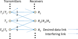
Figure 1: Example of a B-MAC network

Note that when DPC and SIC are combined, an interference may not be fully cancelled under a specific encoding and decoding order. Such case cannot be described by the coupling matrix of 0’s and 1’s defined above. But a valid coupling matrix can serve for an upper or lower bound. See more discussion in [1].

If not explicitly stated otherwise, achievable regions in this paper refer to the following. Note that $\mathbf{\Phi}_{l,l}=0$ by definition. The interference-plus-noise covariance matrix of the $l^{\text{th}}$ link is

$$\mathbf{\Omega}_{l} = \mathbf{I}+\sum_{k=1}^{L}\mathbf{\Phi}_{l,k}\mathbf{H}_{l,k}\mathbf{\Sigma}_{k}\mathbf{H}_{l,k}^{\dagger},$$ (2)

where $\mathbf{\Sigma}_{k}$ is the covariance matrix of $\mathbf{x}_{k}$. We denote all the covariance matrices as

$$\mathbf{\Sigma}_{1:L} = \left(\mathbf{\Sigma}_{1},\mathbf{\Sigma}_{2},...,\mathbf{\Sigma}_{L}\right).$$ (3)

Then the achievable mutual information (rate) of link $l$ is given by a function of $\mathbf{\Sigma}_{1:L}$ and $\mathbf{\Phi}$

$$\mathcal{I}_{l}\left(\mathbf{\Sigma}_{1:L},\mathbf{\Phi}\right) = \textrm{log}\left|\mathbf{I}+\mathbf{H}_{l,l}\mathbf{\Sigma}_{l}\mathbf{H}_{l,l}^{\dagger}\mathbf{\Omega}_{l}^{-1}\right|.$$ (4)

Definition 1

The Achievable Rate Region with a fixed coupling matrix $\mathbf{\Phi}$ and sum power constraint $P_{T}$ is defined as

$$\mathcal{R}_{\mathbf{\Phi}}\left(P_{T}\right) \triangleq \underset{\mathbf{\Sigma}_{1:L}:\sum_{l=1}^{L}\textrm{Tr}\left(\mathbf{\mathbf{\Sigma}}_{l}\right)\leq P_{T}}{\bigcup}\left\{\mathbf{r}\in\mathbb{R}_{+}^{L}:\right.$$

$$\left.r_{l}\leq\mathcal{I}_{l}\left(\mathbf{\Sigma}_{1:L},\mathbf{\Phi}\right),1\leq l\leq L\right\}.$$

A bigger achievable rate region can be defined by the convex closure of $\bigcup_{\mathbf{\Phi}\in\mathbf{\Xi}}\mathcal{R}_{\mathbf{\Phi}}\left(P_{T}\right)$, where $\mathbf{\Xi}$ is a set of valid coupling matrices. For example, if DPC and/or SIC are employed, $\mathbf{\Xi}$ can be a set of valid coupling matrices corresponding to various valid encoding and/or decoding orders.

The algorithms rely on the duality between the forward and reverse links of a B-MAC network. The reverse links are obtained by reversing the transmission direction and replacing the channel matrices by their conjugate transposes. The coupling matrix for the reverse links is the transpose of that for the forward links. We use the notation $\hat{}$ to denote the corresponding terms in the reverse links. For example, in the reverse links of the B-MAC network in Fig. 1, $T_{1}/T_{2}$ ($R_{2}/R_{3}$) becomes the receiver (transmitter), and $\mathbf{\hat{x}}_{2}$ is decoded after $\hat{\mathbf{x}}_{1}$ and $\mathbf{\hat{x}}_{3}$ is encoded after $\hat{\mathbf{x}}_{2}$, if in the forward links, $\mathbf{x}_{1}$ is encoded after $\mathbf{x}_{2}$ and $\mathbf{x}_{2}$ is decoded after $\mathbf{x}_{3}$. The interference-plus-noise covariance matrix of reverse link $l$ is

$$\hat{\mathbf{\Omega}}_{l} = \mathbf{I}+\sum_{k=1}^{L}\mathbf{\Phi}_{k,l}\mathbf{H}_{k,l}^{\dagger}\mathbf{\hat{\mathbf{\Sigma}}}_{k}\mathbf{H}_{k,l},$$ (6)

and the rate of reverse link $l$ is given by $\mathcal{\hat{I}}_{l}\left(\hat{\mathbf{\Sigma}}_{1:L},\mathbf{\Phi}^{T}\right)=\textrm{log}\left|\mathbf{I}+\mathbf{H}_{l,l}^{\dagger}\hat{\mathbf{\Sigma}}_{l}\mathbf{H}_{l,l}\hat{\mathbf{\Omega}}_{l}^{-1}\right|.$

II-B Problem Formulation

This paper concerns the feasibility optimization problem (FOP) and the sum power minimization problem (SPMP) under Quality of Service (QoS) constraints in terms of target rates $\left[\mathcal{I}_{l}^{0}\right]_{l=1,...,L}$ for a B-MAC network with a given valid coupling matrix $\mathbf{\Phi}$:

FOP: $$\underset{\mathbf{\Sigma}_{1:L}}{\textrm{max}} \left(\min_{1\leq l\leq L}\frac{\mathcal{I}_{l}\left(\mathbf{\Sigma}_{1:L},\mathbf{\Phi}\right)}{\mathcal{I}_{l}^{0}}\right)$$

s.t. $$\mathbf{\Sigma}_{l}\succeq 0,l=1,...,L\>\textrm{and}\>\sum_{l=1}^{L}\textrm{Tr}\left(\mathbf{\Sigma}_{l}\right)\leq P_{T},$$

where $P_{T}$ is the total power constraint;

SPMP: $$\underset{\mathbf{\Sigma}_{1:L}}{\textrm{min}} \sum_{l=1}^{L}\textrm{Tr}\left(\mathbf{\Sigma}_{l}\right)$$

s.t. $$\mathcal{I}_{l}\left(\mathbf{\Sigma}_{1:L},\mathbf{\Phi}\right)\geq\mathcal{I}_{l}^{0},\mathbf{\Sigma}_{l}\succeq 0,l=1,...,L.$$

In FOP, if the optimum of the objective function is $\alpha$ and is greater than one, the target rates are feasible. The optimum input covariance matrices achieves a point on the boundary of the achievable region along the direction of vector $\left[\mathcal{I}_{l}^{0}\right]_{l=1,...,L}$, i.e., the optimal rate vector satisfies $\left[\mathcal{I}_{l}\right]_{l=1,...,L}=\alpha\left[\mathcal{I}_{l}^{0}\right]_{l=1,...,L}$. If the target rates is feasible for some power, SPMP finds the minimum total power needed. For the special case of DPC and SIC, the optimal coupling matrix $\mathbf{\Phi}$, or equivalently, the optimal encoding and/or decoding order of FOP and SPMP is partially solved in Section IV-G. We first focus on centralized algorithms under total power constraints. Then we give a distributed implementation of the algorithm for SPMP under additional individual maximum power constraints.

Although we focus on the sum power and white noise in this paper for simplicity, the results can be directly applied to a much larger class of problems with a single linear constraint $\sum_{l=1}^{L}\textrm{Tr}\left(\mathbf{\Sigma}_{l}\hat{\mathbf{W}}_{l}\right)\leq P_{T}$ in FOP (or objective function $\sum_{l=1}^{L}\textrm{Tr}\left(\mathbf{\Sigma}_{l}\hat{\mathbf{W}}_{l}\right)$ in SPMP) and/or colored noise with covariance $\text{E}\left[\mathbf{w}_{l}\mathbf{\mathbf{w}}_{l}^{\dagger}\right]=\mathbf{W}_{l}$, which includes the weighted sum power minimization problem in [10] as a special case. Only variable changes $\mathbf{\Sigma}_{l}^{\prime}=\hat{\mathbf{W}}_{l}^{\frac{1}{2}}\mathbf{\Sigma}_{l}\hat{\mathbf{W}}_{l}^{\frac{1}{2}}$ and $\mathbf{W}_{k}^{-\frac{1}{2}}\mathbf{H}_{k,l}\hat{\mathbf{W}}_{l}^{-\frac{1}{2}}$ are needed, where $\hat{\mathbf{W}}_{l}$ and $\mathbf{W}_{k}$ are positive definite for meaningful cases. The single linear constraint appears in Lagrange functions for problems with multiple linear constraints [23, 24], and thus, the results in this paper serve as the basis to solve them [25]. Special cases of multiple linear constraints include individual power constraints, per-antenna power constraints, interference constraints in cognitive radios, etc..

III Preliminaries

The algorithms are based on SINR duality, e.g., [10], rate duality, and polite water-filling developed earlier [1]. They are reviewed below.

III-A SINR Duality for MIMO B-MAC Networks

The achievable rate region defined in (II-A) can be achieved by a spatial multiplexing scheme as follows.

Definition 2

The Decomposition of a MIMO Link into Multiple SISO Data Streams is defined as, for link $l$ and $M_{l}\geq\text{Rank}(\mathbf{\Sigma}_{l})$, finding a precoding matrix $\dot{\mathbf{T}}_{l}=\left[\sqrt{p_{l,1}}\mathbf{t}_{l,1},...,\sqrt{p_{l,M_{l}}}\mathbf{t}_{l,M_{l}}\right]$ satisfying

$$\mathbf{\Sigma}_{l}=\dot{\mathbf{T}}_{l}\dot{\mathbf{T}}_{l}^{\dagger}=\sum_{m=1}^{M_{l}}p_{l,m}\mathbf{t}_{l,m}\mathbf{t}_{l,m}^{\dagger},$$ (9)

where $\mathbf{t}_{l,m}\in\mathbb{C}^{L_{T_{l}}\times 1}$ is a transmit vector with $\left\|\mathbf{t}_{l,m}\right\|=1$; and $\mathbf{p}=\left[p_{1,1},...,p_{1,M_{1}},...,p_{L,1},...,p_{L,M_{L}}\right]^{T}$ are the transmit powers.

Note that the precoding matrix is not unique because $\dot{\mathbf{T}}_{l}^{{}^{\prime}}=\dot{\mathbf{T}}_{l}\mathbf{V}$ with unitary $\mathbf{V}\in\mathbb{C}^{M_{l}\times M_{l}}$ also gives the same covariance matrix in (9). Without loss of generality, we assume the intra-signal decoding order is that the $m^{\text{th}}$ stream is the $m^{\text{th}}$ to be decoded and cancelled. The receive vector for the $m^{th}$ stream of link $l$ is obtained by the MMSE filtering as

$$\mathbf{r}_{l,m}=\alpha_{l,m}\left(\sum_{i=m+1}^{M_{l}}\mathbf{H}_{l,l}p_{l,i}\mathbf{t}_{l,i}\mathbf{t}_{l,i}^{\dagger}\mathbf{H}_{l,l}^{\dagger}+\mathbf{\Omega}_{l}\right)^{-1}\mathbf{H}_{l,l}\mathbf{t}_{l,m},$$ (10)

where $\alpha_{l,m}$ is chosen such that $\left\|\mathbf{r}_{l,m}\right\|=1$. This is referred to as MMSE-SIC receiver in this paper.

For each stream, one can calculate its SINR. Let the collections of transmit and receive vectors be

$$\mathbf{T} = \left[\mathbf{t}_{l,m}\right]_{m=1,...,M_{l},l=1,...,L},$$ (11)

$$\mathbf{R} = \left[\mathbf{r}_{l,m}\right]_{m=1,...,M_{l},l=1,...,L}.$$ (12)

The cross-talk matrix $\mathbf{\Psi}\left(\mathbf{T},\mathbf{R}\right)\in\mathbb{R}_{+}^{\sum_{l}M_{l}\times\sum_{l}M_{l}}$ between different streams [8] is a function of $\mathbf{T},\mathbf{R}$, and, assuming unit transmit power, the element of the $\left(\sum_{i=1}^{l-1}M_{i}+m\right)^{\textrm{th}}$ row and $\left(\sum_{i=1}^{k-1}M_{i}+n\right)^{\textrm{th}}$ column of $\mathbf{\Psi}$ is the interference power from the $k^{\text{th}}$ link’s $n^{\text{th}}$ stream to the $l^{\text{th}}$ link’s $m^{\text{th}}$ stream and is given by

$$\mathbf{\Psi}_{l,m}^{k,n}= \begin{cases}0&k=l\>\textrm{and}\>m\geq n,\\ \left|\mathbf{r}_{l,m}^{\dagger}\mathbf{H}_{l,l}\mathbf{t}_{l,n}\right|^{2}&k=l,\>\textrm{and}\>m<n,\\ \Phi_{l,k}\left|\mathbf{r}_{l,m}^{\dagger}\mathbf{H}_{l,k}\mathbf{t}_{k,n}\right|^{2}&\textrm{otherwise}.\end{cases}$$ (13)

Then the SINR for the $m^{th}$ stream of link $l$ is

$$\gamma_{l,m}\left(\mathbf{T},\mathbf{R},\mathbf{p}\right) = \frac{p_{l,m}\left|\mathbf{r}_{l,m}^{\dagger}\mathbf{H}_{l,l}\mathbf{t}_{l,m}\right|^{2}}{1+{\displaystyle\sum_{k=1}^{L}}{\displaystyle\sum_{n=1}^{M_{k}}}p_{k,n}\mathbf{\Psi}_{l,m}^{k,n}}.$$ (14)

Such decomposition of data to streams with MMSE-SIC receiver is information lossless [26], i.e., the sum-rate of all streams of link $l$ is equal to the mutual information in (4).

In the reverse links, we can obtain SINRs using $\mathbf{R}$ as transmit vectors and $\mathbf{T}$ as receive vectors. The transmit powers are denoted as $\mathbf{q}=\left[q_{1,1},...,q_{1,M_{1}},...,q_{L,1},...,q_{L,M_{L}}\right]^{T}$. The intra-signal decoding order is the opposite to that of the forward link, i.e., the $m^{\text{th}}$ stream is the $m^{\text{th}}$ last to be decoded and cancelled. Then the SINR for the $m^{th}$ stream of reverse link $l$ is

$$\hat{\gamma}_{l,m}\left(\mathbf{R},\mathbf{T},\mathbf{q}\right) = \frac{q_{l,m}\left|\mathbf{t}_{l,m}^{\dagger}\mathbf{H}_{l,l}^{\dagger}\mathbf{r}_{l,m}\right|^{2}}{1+{\displaystyle\sum_{k=1}^{L}}{\displaystyle\sum_{n=1}^{M_{k}}}q_{k,n}\mathbf{\Psi}_{k,n}^{l,m}}.$$ (15)

For simplicity, we will use $\left\{\mathbf{T},\mathbf{R},\mathbf{p}\right\}$ ($\left\{\mathbf{R},\mathbf{T},\mathbf{q}\right\}$) to denote the transmission and reception strategy described above in the forward (reverse) links.

The achievable SINR regions of the forward and reverse links are the same. Define the achievable SINR regions $\mathcal{T}_{\mathbf{\Phi}}\left(P_{T}\right)$ and $\mathcal{\hat{T}}_{\mathbf{\Phi}^{T}}\left(P_{T}\right)$ as the set of all SINRs that can be achieved under the sum power constraint $P_{T}$ in the forward and reverse links respectively. For a given set of SINR values $\mathbf{\gamma}^{0}=\left[\gamma_{l,m}^{0}\right]_{m=1,...,M_{l},l=1,...,L}$, define a diagonal matrix $\mathbf{D}\left(\mathbf{T},\mathbf{R},\mathbf{\gamma}^{0}\right)\in\mathbb{R}_{+}^{\sum_{l}M_{l}\times\sum_{l}M_{l}}$ where the $\left(\sum_{i=1}^{l-1}M_{i}+m\right)^{\text{th}}$ diagonal element is

$$\mathbf{D}_{\sum_{i=1}^{l-1}M_{i}+m,\sum_{i=1}^{l-1}M_{i}+m} = \gamma_{l,m}^{0}/\left|\mathbf{r}_{l,m}^{\dagger}\mathbf{H}_{l,l}\mathbf{t}_{l,m}\right|^{2}.$$ (16)

We restate the SINR duality, e.g. [10], as follows.

Lemma 1

If a set of SINRs $\mathbf{\gamma}^{0}$ is achieved by the transmission and reception strategy $\left\{\mathbf{T},\mathbf{R},\mathbf{p}\right\}$ with $\left\|\mathbf{p}\right\|_{1}=P_{T}$ in the forward links, then $\mathbf{\gamma}^{0}$ is also achievable in the reverse links with $\left\{\mathbf{R},\mathbf{T},\mathbf{q}\right\}$, where $\mathbf{q}$ satisfies $\left\|\mathbf{q}\right\|_{1}=P_{T}$ and is given by

$$\mathbf{q} = \left(\mathbf{D}^{-1}\left(\mathbf{T},\mathbf{R},\mathbf{\gamma}^{0}\right)-\mathbf{\Psi}^{T}\left(\mathbf{T},\mathbf{R}\right)\right)^{-1}\mathbf{1}.$$ (17)

And thus, one has $\mathcal{T}_{\mathbf{\Phi}}\left(P_{T}\right)=\mathcal{\hat{T}}_{\mathbf{\Phi}^{T}}\left(P_{T}\right)$.

III-B Rate Duality

The rate duality of the forward and reverse links of the B-MAC networks is a simple consequence of the SINR duality [1]. The reverse link input covariance matrices are obtained by the following transformation.

Definition 3

Let $\mathbf{\Sigma}_{l}=\sum_{m=1}^{M_{l}}p_{l,m}\mathbf{t}_{l,m}\mathbf{t}_{l,m}^{\dagger},l=1,...,L$ be a decomposition of $\mathbf{\Sigma}_{1:L}$. Compute the MMSE-SIC receive vectors $\mathbf{R}$ from (10) and the reverse transmit powers $\mathbf{q}$ from (17). The Covariance Transformation from $\mathbf{\Sigma}_{1:L}$ to $\hat{\mathbf{\Sigma}}_{1:L}$ is

$$\hat{\mathbf{\Sigma}}_{l} = \sum_{m=1}^{M_{l}}q_{l,m}\mathbf{r}_{l,m}\mathbf{r}_{l,m}^{\dagger},l=1,...,L.$$ (18)

We give the rate duality under a linear constraint $\sum_{l=1}^{L}\textrm{Tr}\left(\mathbf{\Sigma}_{l}\hat{\mathbf{W}}_{l}\right)\leq P_{T}$ and/or colored noise with covariance $\text{E}\left[\mathbf{w}_{l}\mathbf{\mathbf{w}}_{l}^{\dagger}\right]=\mathbf{W}_{l}$. The covariance transformation for this case is also calculated from the MMSE receive beams and power allocation that makes SINRs of the forward and reverse links equal, as in (18). The only difference is that the identity noise covariance in $\mathbf{\Omega}_{l}$ is replaced by $\mathbf{W}_{l}$ and the all-one vector $\mathbf{1}$ in (17) is replaced by the vector $\left[\mathbf{t}_{l,m}^{\dagger}\hat{\mathbf{W}}_{l}\mathbf{t}_{l,m}\right]_{m=1,...,M_{l},l=1,...,L}$. For convenience, let

$$\left(\left[\mathbf{H}_{l,k}\right],\sum_{l=1}^{L}\textrm{Tr}\left(\mathbf{\Sigma}_{l}\hat{\mathbf{W}}_{l}\right)\leq P_{T},\left[\mathbf{W}_{l}\right]\right),$$ (19)

denote a network where the channel matrices are $\left[\mathbf{H}_{l,k}\right]$; the input covariance matrices must satisfy the linear constraint $\sum_{l=1}^{L}\textrm{Tr}\left(\mathbf{\Sigma}_{l}\hat{\mathbf{W}}_{l}\right)\leq P_{T}$; and the covariance matrix of the noise at the receiver of link $l$ is $\mathbf{W}_{l}$. Then the rate duality is restated in the theorem below.

Theorem 1

The dual of the network (19) is

$$\left(\left[\mathbf{H}_{k,l}^{\dagger}\right],\sum_{l=1}^{L}\textrm{Tr}\left(\hat{\mathbf{\Sigma}}_{l}\mathbf{W}_{l}\right)\leq P_{T},\left[\hat{\mathbf{W}}_{l}\right]\right)$$ (20)

in the sense that 1) they have the same achievable rate region; 2) if $\mathbf{\Sigma}_{1:L}$ achieves certain rates and satisfies the linear constraint in network (19), its covariance transformation $\hat{\mathbf{\Sigma}}_{1:L}$ achieves better rates in network (20) under the linear constraint $\sum_{l=1}^{L}\textrm{Tr}\left(\hat{\mathbf{\Sigma}}_{l}\mathbf{W}_{l}\right)=\sum_{l=1}^{L}\textrm{Tr}\left(\mathbf{\Sigma}_{l}\hat{\mathbf{W}}_{l}\right)\leq P_{T}$.

III-C Polite Water-filling

In [1], we showed that the Pareto optimal input covariance matrices have a polite water-filling structure, which is defined below. It generalizes the well known optimal single user water-filling structure to networks.

Definition 4

Given input covariance matrices $\mathbf{\Sigma}_{1:L}$, obtain its covariance transformation $\hat{\mathbf{\Sigma}}_{1:L}$ as in (18). Let $\mathbf{\Omega}_{l}$’s and $\hat{\mathbf{\Omega}}_{l}$’s respectively be the corresponding interference-plus-noise covariance matrices. For each link $l$, pre- and post- whiten the channel $\mathbf{H}_{l,l}$ to produce an equivalent single user channel $\bar{\mathbf{H}}_{l}=\mathbf{\Omega}_{l}^{-1/2}\mathbf{H}_{l,l}\hat{\mathbf{\Omega}}_{l}^{-1/2}$. Define $\mathbf{Q}_{l}\triangleq\hat{\mathbf{\Omega}}_{l}^{1/2}\mathbf{\Sigma}_{l}\hat{\mathbf{\Omega}}_{l}^{1/2}$ as the equivalent input covariance matrix of link $l$. The input covariance matrix $\mathbf{\Sigma}_{l}$ is said to possess a polite water-filling structure if $\mathbf{Q}_{l}$ satisfies the structure of water-filling over $\bar{\mathbf{H}}_{l}$, i.e.,

$$\mathbf{Q}_{l} = \mathbf{G}_{l}\mathbf{D}_{l}\mathbf{G}_{l}^{\dagger},$$ (21)

$$\mathbf{D}_{l} = \left(\nu_{l}\mathbf{I}-\mathbf{\Delta}_{l}^{-2}\right)^{+}.$$

where $\nu_{l}\geq 0$ is called the polite water-filling level; the equivalent channel $\bar{\mathbf{H}}_{l}$’s thin singular value decomposition (SVD) is $\bar{\mathbf{H}}_{l}=\mathbf{F}_{l}\mathbf{\Delta}_{l}\mathbf{G}_{l}^{\dagger}$ with $\mathbf{F}_{l}\in\mathbb{C}^{L_{R_{l}}\times N_{l}},\ \mathbf{G}_{l}\in\mathbb{C}^{L_{T_{l}}\times N_{l}},\ \mathbf{\Delta}_{l}\in\mathbb{R}_{++}^{N_{l}\times N_{l}}$, and $N_{l}=\textrm{Rank}\left(\mathbf{H}_{l,l}\right)$. If all $\mathbf{\Sigma}_{l}$’s possess the polite water-filling structure, then $\mathbf{\Sigma}_{1:L}$ is said to possess the polite water-filling structure.

Theorem 2

The input covariance matrices $\mathbf{\Sigma}_{1:L}$ of a Pareto rate point of the achievable region and its covariance transformation $\hat{\mathbf{\Sigma}}_{1:L}$ possess the polite water-filling structure.

The following theorem proved in [1] states that $\mathbf{\Sigma}_{l}$ having the polite water-filling structure suffices for $\hat{\mathbf{\Sigma}}_{l}$ to have the polite water-filling structure even at a non-Pareto rate point.

Theorem 3

If one input covariance matrix $\mathbf{\Sigma}_{l}$ has the polite water-filling structure while other $\mathbf{\Sigma}_{k},\hat{\mathbf{\Sigma}}_{k},$ $k\neq l,$ are fixed, so does its covariance transformation $\hat{\mathbf{\Sigma}}_{l}$, i.e., $\mathbf{\hat{Q}}_{l}\triangleq\mathbf{\Omega}_{l}^{1/2}\hat{\mathbf{\Sigma}}_{l}\mathbf{\Omega}_{l}^{1/2}$ satisfies the structure of water-filling over the reverse equivalent channel $\bar{\mathbf{H}}_{l}^{\dagger}\triangleq\hat{\mathbf{\Omega}}_{l}^{-1/2}\mathbf{H}_{l,l}^{\dagger}\mathbf{\Omega}_{l}^{-1/2}$. Further more, $\hat{\mathbf{\Sigma}}_{l}$ can be expressed as

$$\hat{\mathbf{\Sigma}}_{l} =\nu_{l}\left(\mathbf{\Omega}_{l}^{-1}-\left(\mathbf{H}_{l,l}\mathbf{\Sigma}_{l}\mathbf{H}_{l,l}^{\dagger}+\mathbf{\Omega}_{l}\right)^{-1}\right),\ l=1,...,L,$$ (22)

where $\nu_{l}$ is the polite water-filling level in (21).

IV Optimization Algorithms

In this section, we present several related algorithms for the feasibility optimization problem (FOP) and the sum power minimization problem (SPMP) under rate constraints. SINR based and polite water-filling based algorithms are designed. Algorithms for SINR version of FOP and SPMP have been designed in [8, 10]. To take advantage of them, we show how to map a Pareto point of the achievable rate region to a Pareto point of the SINR region in Section IV-A and then use SINR based Algorithm A and B to solve FOP and SPMP respectively in Section IV-B. The optimality of Algorithms A and B is studied in Section IV-C by examining the structure of the optimal solutions of FOP and SPMP. Then, for iTree networks defined later, Algorithm I is designed to improve the output of Algorithm A and B. The improvement and the optimal structure suggests that the rate constrained problems can be directly solved using Algorithm PR and PR1 in Section IV-E by polite water-filling, without resorting to the SINR based approach. In a network, it is desirable to have distributed algorithms, for which Algorithm PRD is designed in Section IV-F. Finally, we design Algorithm O to improve the encoding and decoding orders for all of the above algorithms when DPC and SIC are employed. For convenience, a list of algorithms in this paper is summarized in Table I.

Table I: List of Algorithms

Sec.	Tab.	Alg.	Purpose
IV-B	II	A	SINR based, for EFOP
IV-B	III	B	SINR based, for ESPMP
IV-D	IV	S	Subroutine, for link $i$
IV-D	V	I	Improvement of A/B for iTree networks
IV-E	VI	W	Subroutine, for water-filling level
IV-E	VII	PR	Polite WF based, for iTree, SPMP
IV-E	VIII	PR1	Polite WF based, for B-MAC, SPMP
IV-F	IX	PRD	Distributed version of PR1
IV-G	X	O	Enc./dec. order optimization, for FOP/SPMP

IV-A Rate-SINR Conversion

In order to find Pareto rate points of the achievable rate region by taking advantage of algorithms that finds Pareto points of the SINR region, one needs to find a mapping from a Pareto rate point to a Pareto SINR point. But multiple SINR points can correspond to the same rate and thus, multiple mappings exist. The following two theorems give an equal SINR mapping and an equal power mapping by choosing two decompositions of a MIMO link to multiple SISO data streams. Note that for the same total link rate, different decompositions have different sets of SINRs of the streams and different number of streams. We show that equal SINR allocation or equal power allocation among the streams within a link will not lose optimality.

Theorem 4

For any input covariance matrices $\mathbf{\Sigma}_{1:L}$ achieving a rate point $\left[\mathcal{I}_{l}\right]_{l=1,...,L}$, there exists a decomposition $\mathbf{\Sigma}_{l}=\dot{\mathbf{T}}_{l}\dot{\mathbf{T}}_{l}^{\dagger}=\sum_{m=1}^{M_{l}}p_{l,m}\mathbf{t}_{l,m}\mathbf{t}_{l,m}^{\dagger},l=1,...,L$, with $M_{l}\geq\text{Rank}(\mathbf{\Sigma}_{l})$, such that the corresponding transmission and MMSE-SIC reception strategy $\left\{\mathbf{T},\mathbf{R},\mathbf{p}\right\}$ achieves equal SINR for all streams of the same link, i.e., $\gamma_{l,m}=e^{\mathcal{I}_{l}/M_{l}}-1,m=1,...,M_{l},l=1,...,L$. Therefore uniform rate allocation over the streams of the same link will not lose optimality.

The proof is given in appendix -A and provides an algorithm to find the decomposition. An immediate consequence of Theorem 4 is a mapping of the Pareto boundary points of the achievable rate region to the SINR region.

Corollary 1

Let $M_{l}=\text{Rank}(\mathbf{H}_{l,l})$. An SINR point $\left[\gamma_{l,m}=e^{\mathcal{I}_{l}/M_{l}}-1\right]_{m=1,...,M_{l},l=1,...,L}$ is a Pareto boundary point in $\mathcal{T}_{\mathbf{\Phi}}\left(P_{T}\right)$, if and only if the rate point $\left[\mathcal{I}_{l}\right]_{l=1,...,L}$ is a Pareto rate point in $\mathcal{R}_{\mathbf{\Phi}}\left(P_{T}\right)$.

Therefore, the problem with rate constraints $\left[\mathcal{I}_{l}^{0}\right]_{l=1,...,L}$ can be equivalently solved through the problem with SINR constraints $\left[\gamma_{l,m}=e^{\mathcal{I}_{l}/M_{l}}-1\right]_{m=1,...,M_{l},l=1,...,L}$.

The following theorem shows that uniform power allocation across the streams within a link will also not lose optimality, which is useful in designing algorithms for individual power constraints and/or distributed optimization [27, 28].

Theorem 5

For any input covariance matrix $\mathbf{\Sigma}$, there exists a decomposition $\mathbf{\Sigma}=\sum_{m=1}^{M}p_{m}\mathbf{t}_{m}\mathbf{t}_{m}^{\dagger}$ such that the transmit power is uniformly allocated over the $M$ streams, i.e., $p_{m}=\textrm{Tr}\left(\mathbf{\Sigma}\right)/M,\forall m$. Therefore uniform power allocation over the streams of the same link will not lose optimality.

The proof is given in Appendix -B.

IV-B SINR based Algorithms

The results in Section IV-A serve as a bridge to solve the FOP or SPMP under rate constraints through the SINR optimization problems. First we show FOP is equivalent to the following SINR optimization problem in the sense of feasibility.

$$\textrm{{EFOP}}:\underset{\left\{\mathbf{T},\mathbf{R},\mathbf{p}\right\}}{\textrm{max}} \min_{\begin{array}[]{c}1\leq m\leq M_{l}\\ 1\leq l\leq L\end{array}}\frac{\gamma_{l,m}}{\gamma_{l}^{0}},\>\textrm{s.t.}\left\|\mathbf{p}\right\|_{1}\leq P_{T}$$ (25)

where $M_{l}=\textrm{Rank}\left(\mathbf{H}_{l,l}\right)$ is the number of streams of link $l$; $\gamma_{l}^{0}=e^{\mathcal{I}_{l}^{0}/M_{l}}-1$ is the target SINR for the streams of link $l$.

Theorem 6

The optimum of FOP (II-B) is not less than 1 if and only if the optimum of EFOP (25) is not less than 1.

Proof:

If the optimum of EFOP is not less than 1, there exists a point $\left[\gamma_{l,m}\geq\gamma_{l}^{0}\right]_{m=1,...,M_{l},l=1,...,L}$ in $\mathcal{T}_{\mathbf{\Phi}}\left(P_{T}\right)$. Then it follows from Corollary 1 that the rate point $\left[\mathcal{I}_{l}=M_{l}\textrm{log}\left(1+\gamma_{l,m}\right)\geq\mathcal{I}_{l}^{0}\right]_{l=1,...,L}$ lies in $\mathcal{R}_{\mathbf{\Phi}}\left(P_{T}\right)$, i.e., the optimum of FOP is not less than 1. The ’only if’ part can be proved similarly. ∎

Remark 1

If the target rates $\left(\mathcal{I}_{1}^{0},...,\mathcal{I}_{L}^{0}\right)$ is not a Pareto point but feasible, the solution of EFOP may produce a Pareto rate point that is not a solution of the FOP. However, both will exceed the target rates.

Similarly, SPMP is equivalent to the following SINR optimization problem

$$\textrm{{ESPMP}}:\underset{\left\{\mathbf{T},\mathbf{R},\mathbf{p}\right\}}{\textrm{min}}\left\|\mathbf{p}\right\|_{1},\>\textrm{s.t.}\>\gamma_{l,m}\geq\gamma_{l}^{0},\begin{array}[]{c}1\leq m\leq M_{l},\\ 1\leq l\leq L.\end{array}$$ (26)

Theorem 7

If $\left\{\tilde{\mathbf{T}},\tilde{\mathbf{R}},\tilde{\mathbf{p}}\right\}$ is an optimum of ESPMP (26), the input covariance matrices $\tilde{\mathbf{\Sigma}}_{1:L}$ produced by $\tilde{\mathbf{T}}$ and $\tilde{\mathbf{p}}$ must be an optimum of SPMP (II-B). On the other hand, if $\tilde{\mathbf{\Sigma}}_{1:L}$ is an optimum of SPMP, there exists a decomposition leading to $\left\{\tilde{\mathbf{T}},\tilde{\mathbf{R}},\tilde{\mathbf{p}}\right\}$, which is an optimum of ESPMP.

Proof:

If $\tilde{\mathbf{\Sigma}}_{1:L}$ produced by $\tilde{\mathbf{T}}$ and $\tilde{\mathbf{p}}$ is not an optimum of SPMP, there exists a solution $\mathbf{\Sigma}_{1:L}^{{}^{\prime}}$ such that $\left[\mathcal{I}_{l}^{0}\right]_{l=1,...,L}$ can be achieved by a smaller total transmit power. Then it follows from Theorem 4 that there exists a decomposition of $\mathbf{\Sigma}_{1:L}^{{}^{\prime}}$ such that the target SINRs $\left[\gamma_{l,m}^{0}=e^{\mathcal{I}_{l}^{0}/M_{l}}-1\right]_{m=1,...,M_{l},l=1,...,L}$ are achieved by the corresponding $\left\{\mathbf{T}^{{}^{\prime}},\mathbf{R}^{{}^{\prime}},\mathbf{p}^{{}^{\prime}}\right\}$ with $\left\|\mathbf{p}^{{}^{\prime}}\right\|_{1}<\left\|\mathbf{\tilde{p}}\right\|_{1}$, which contradicts with the optimality of $\left\{\tilde{\mathbf{T}},\tilde{\mathbf{R}},\tilde{\mathbf{p}}\right\}$. The reverse part can be proved similarly.∎

Remark 2

It is possible that neither SPMP nor ESPMP is feasible, i.e., the target rates or SINRs can not be achieved even with infinite power. In this paper, we only consider feasible problems. In practice, we can avoid solving the infeasible SPMP and ESPMP by solving the FOP with the maximum allowable sum power to test the feasibility first.

By converting the FOP and SPMP to the simpler EFOP and ESPMP, these problems can be efficiently solved by the SINR duality based algorithms for MIMO beamforming networks [8, 10], which is summarized below. For fixed $\mathbf{T},\mathbf{p}$, the optimal receive vector for each stream is decoupled and is given by the MMSE-SIC receiver in (10). The SINR duality in Lemma 1 implies that the coupled problem of optimizing the transmit vectors can be found by optimizing the receive vectors in the reverse links, i.e., for fixed $\mathbf{R},\mathbf{q}$, the optimal receive vector for each stream in the reverse links is given by the MMSE-SIC receiver

$$\mathbf{t}_{l,m} =\beta_{l,m}\left(\sum_{i=1}^{m-1}q_{l,i}\mathbf{H}_{l,l}^{\dagger}\mathbf{r}_{l,i}\mathbf{r}_{l,i}^{\dagger}\mathbf{H}_{l,l}+\hat{\mathbf{\Omega}}_{l}\right)^{-1}\mathbf{H}_{l,l}^{\dagger}\mathbf{r}_{l,m}$$ (27)

where $\hat{\mathbf{\Omega}}_{l}$ is obtained from $\hat{\mathbf{\Sigma}}_{k}=\sum_{i=1}^{M_{k}}q_{k,i}\mathbf{r}_{k,i}\mathbf{r}_{k,i}^{\dagger},\ k\neq l$ using (6), and $\beta_{l,m}$ is chosen such that $\left\|\mathbf{t}_{l,m}\right\|=1$.

The optimization for $\mathbf{p}$ is different for the two problems. The algorithm designed in [8] for EFOP is described below. For fixed $\mathbf{T},\mathbf{R}$, define the following extended coupling matrices [8]

$$\mathbf{\Upsilon} = \left[\begin{array}[]{cc}\mathbf{D}\mathbf{\Psi}&\mathbf{D}\mathbf{1}\\ \frac{1}{P_{T}}\mathbf{1}^{T}\mathbf{D}\mathbf{\Psi}&\frac{1}{P_{T}}\mathbf{1}^{T}\mathbf{D}\mathbf{1}\end{array}\right],$$ (30)

$$\mathbf{\mathbf{\Lambda}} = \left[\begin{array}[]{cc}\mathbf{D}\mathbf{\Psi}{}^{T}&\mathbf{D}\mathbf{1}\\ \frac{1}{P_{T}}\mathbf{1}^{T}\mathbf{D}\mathbf{\Psi}{}^{T}&\frac{1}{P_{T}}\mathbf{1}^{T}\mathbf{D}\mathbf{1}\end{array}\right],$$ (33)

where $\mathbf{\Psi}$ and $\mathbf{D}$ are defined in (13) and (16) respectively; and the SINR values in $\mathbf{D}$ are fixed as $\gamma_{l,m}^{0}=\gamma_{l}^{0},m=1,...,M_{l},l=1,...,L$, where $\gamma_{l}^{0}$’s are the target SINRs in EFOP. With the optimal power $\mathbf{\tilde{p}}$, all the scaled SINRs in (25) should be equal to the same value denoted as $C_{\textrm{max}}$ [8]. Therefore $\mathbf{\tilde{p}}$ satisfies the equations $\gamma_{l,m}=C_{\textrm{max}}\gamma_{l}^{0},m=1,...,M_{l},l=1,...,L$ and $\left\|\tilde{\mathbf{p}}\right\|_{1}=P_{T}$, which together form the following eigensystem [8]

$$\mathbf{\mathbf{\Upsilon}}\mathbf{p}_{\textrm{ext}} = \lambda_{\textrm{max}}\mathbf{p}_{\textrm{ext}},$$ (34)

where $\mathbf{p}_{\textrm{ext}}=\left[\mathbf{\tilde{p}}^{T},1\right]^{T}$ is the dominant eigenvector of $\mathbf{\mathbf{\Upsilon}}$ with its last component scaled to one; $\lambda_{\textrm{max}}=1/C_{\textrm{max}}$ is the corresponding maximum eigenvalue. It was proved in [29] that for a non-negative matrix $\mathbf{\Upsilon}$ with the special structure (30), the maximal eigenvalue and its associated eigenvector are strictly positive, and no other eigenvalue fulfills the positivity requirement. Therefore, the last component of $\mathbf{p}_{\textrm{ext}}$ can always be scaled to one and the resulting $\mathbf{\tilde{p}}$ is a valid power vector. Similarly, in the reverse links, the optimal power $\mathbf{\tilde{q}}$ is obtained by solving the eigensystem below [8]

$$\mathbf{\Lambda}\mathbf{q}_{\textrm{ext}}=\hat{\lambda}_{\textrm{max}}\mathbf{q}_{\textrm{ext}},$$ (35)

where $\mathbf{q}_{\textrm{ext}}=\left[\mathbf{\tilde{q}}^{T},1\right]^{T}$ is the dominant eigenvector of $\mathbf{\Lambda}$; and $\hat{\lambda}_{\textrm{max}}$ is the corresponding maximum eigenvalue.

For ESPMP, we use the algorithm in [10]. Let $\gamma_{l,m}^{(n)}$ and $\hat{\gamma}_{l,m}^{(n)}$ respectively be the SINR for the $m^{\text{th}}$ stream of the forward and reverse link $l$ after the $n^{\text{th}}$ update. To satisfy the SINR constraints, the standard power control is used to update $\mathbf{p}$ and $\mathbf{q}$ iteratively, where in each iteration, the power of the stream with over-satisfied (unsatisfied) SINR is reduced (increased):

$$p_{l,m}^{(n+1)} = \frac{\gamma_{l}^{0}}{\gamma_{l,m}^{(n)}}p_{l,m}^{(n)},$$ (36)

$$q_{l,m}^{(n+1)} = \frac{\gamma_{l}^{0}}{\hat{\gamma}_{l,m}^{(n)}}q_{l,m}^{(n)}.$$ (37)

For convenience, we rewrite (36) and (37) into vector functions

$$\mathbf{p}^{(n+1)} = \mathbf{I}_{P}\left(\mathbf{p}^{(n)}\right),$$

$$\mathbf{q}^{(n+1)} = \mathbf{I}_{D}\left(\mathbf{q}^{(n)}\right).$$

Table II: Algorithm A (Solving EFOP)

Choose $\mathbf{p}^{(0)}>0$ and $\mathbf{T}^{(0)}$ such that all streams have positive SINR.

Set $n\leftarrow 0$.

While not converge do

1. Update in the forward links

a. Compute $\mathbf{R}^{(n+1)}$ from $\mathbf{p}^{(n)}$ and $\mathbf{T}^{(n)}$ using (10);

b. Compute $\mathbf{\Lambda}$ from $\mathbf{T}^{(n)}$ and $\mathbf{R}^{(n+1)}$;

c. Solve eigensystem (35) for $\mathbf{q}^{(n+1)}$;

2. Update in the reverse links

a. Compute $\mathbf{T}^{(n+1)}$ from $\mathbf{q}^{(n+1)}$ and $\mathbf{R}^{(n+1)}$ using (27);

b. Compute $\mathbf{\mathbf{\Upsilon}}$ from $\mathbf{T}^{(n+1)}$ and $\mathbf{R}^{(n+1)}$;

c. Solve eigensystem (34) for $\mathbf{p}^{(n+1)}$;

$n\leftarrow n+1$;

End

Table III: Algorithm B (Solving ESPMP)

Choose $\mathbf{p}^{(0)}>0$ and $\mathbf{T}^{(0)}$ such that all streams have positive SINR.

Set $n\leftarrow 0$.

While not converge do

1. Update in the forward links

a. Compute $\mathbf{R}^{(n+1)}$ from $\mathbf{p}^{(n)}$ and $\mathbf{T}^{(n)}$ using (10);

b. Update power in the forward links $\mathbf{p}^{(n+1)}=\mathbf{I}_{P}\left(\mathbf{p}^{(n)}\right)$;

c. Let $\left\{\gamma_{l,m}^{0}=\gamma_{l,m}\left(\mathbf{T}^{(n)},\mathbf{R}^{(n+1)},\mathbf{p}^{(n+1)}\right),\textrm{for\>\ all}\>m,l\right\}$;

d. Compute $\mathbf{D}$ and $\mathbf{\Psi}$ from $\mathbf{T}^{(n)}$, $\mathbf{R}^{(n+1)}$ and $\left\{\gamma_{l,m}^{0}\right\}$;

e. Compute $\mathbf{q}^{(n)}=\left(\mathbf{D}^{-1}-\mathbf{\Psi}^{T}\right)^{-1}\mathbf{1}$;

2. Update in the reverse links

a. Compute $\mathbf{T}^{(n+1)}$ from $\mathbf{q}^{(n)}$ and $\mathbf{R}^{(n+1)}$ using (27);

b. Update power in the forward links $\mathbf{q}^{(n+1)}=\mathbf{I}_{D}\left(\mathbf{q}^{(n)}\right)$;

c. Let $\left\{\gamma_{l,m}^{0}=\gamma_{l,m}\left(\mathbf{T}^{(n+1)},\mathbf{R}^{(n+1)},\mathbf{q}^{(n+1)}\right),\textrm{for\>\ all}\>m,l\right\}$;

d. Compute $\mathbf{D}$ and $\mathbf{\Psi}$ from $\mathbf{T}^{(n+1)}$, $\mathbf{R}^{(n+1)}$ and $\left\{\gamma_{l,m}^{0}\right\}$;

e. Compute $\mathbf{p}^{(n+1)}=\left(\mathbf{D}^{-1}-\mathbf{\Psi}\right)^{-1}\mathbf{1}$;

$n\leftarrow n+1$;

End

The algorithms to solve EFOP and ESPMP are summarized in table II and table III respectively. After obtaining $\mathbf{T},\mathbf{R}$ and $\mathbf{p}$, the corresponding input covariance matrices for FOP and SPMP can be easily obtained.

The convergence of these algorithms are proved in [8, 10]. It can be verified that the objective function in EFOP (25) is monotonically increased by Algorithm A [8]. In Algorithm B, once the solution becomes feasible, i.e., all SINR values meet or exceed the minimum requirements, it generates a sequence of feasible solutions with monotonically decreasing sum power [10]. The optimality of these algorithms will be discussed in the next section.

IV-C Optimality Analysis for SINR based Algorithms

Algorithm A or B can find good solutions but may not find the optimum for general B-MAC networks, according to the numeric examples in Section V. But we can still obtain insight of the problem and derive improved algorithms by finding the necessary conditions satisfied by the optimum.

To avoid deriving the necessary conditions with the non-differentiable objective function of FOP (II-B), we rewrite it into the following equivalent problem

FOPa: $$\underset{\mathbf{\Sigma}_{1:L}}{\textrm{max}} \frac{\mathcal{I}_{1}\left(\mathbf{\Sigma}_{1:L},\mathbf{\Phi}\right)}{\mathcal{I}_{1}^{0}}$$

s.t. $$\frac{\mathcal{I}_{l}\left(\mathbf{\Sigma}_{1:L},\mathbf{\Phi}\right)}{\mathcal{I}_{l}^{0}}\geq\frac{\mathcal{I}_{1}\left(\mathbf{\Sigma}_{1:L},\mathbf{\Phi}\right)}{\mathcal{I}_{1}^{0}},\forall l\neq 1$$

$$\mathbf{\Sigma}_{l}\succeq 0,l=1,\cdots,L\>\textrm{and}\>\sum_{l=1}^{L}\textrm{Tr}\left(\mathbf{\Sigma}_{l}\right)\leq P_{T}.$$

Then the following theorem holds.

Theorem 8

Necessity: If $\tilde{\mathbf{\Sigma}}_{1:L}=\left(\mathbf{\tilde{\mathbf{\Sigma}}}_{1},...,\mathbf{\tilde{\mathbf{\Sigma}}}_{L}\right)$ is an optimum of FOPa (IV-C) or SPMP (II-B), it must satisfy the optimality conditions below:

1. It possesses the polite water-filling structure as in Definition 4.

2. The achieved rates must satisfy $\mathcal{I}_{l}\left(\tilde{\mathbf{\Sigma}}_{1:L},\mathbf{\Phi}\right)=\alpha\mathcal{I}_{l}^{0},l=1,...,L$, where for FOPa, $\alpha>0$ is some constant; and for SPMP, $\alpha=1$.

3. For FOPa, it satisfies $\sum_{l=1}^{L}\textrm{Tr}\left(\tilde{\mathbf{\Sigma}}_{l}\right)=P_{T}$.

On the other hand, if certain $\mathbf{\tilde{\Sigma}}_{1:L}$ satisfies the above optimality conditions for FOPa or SPMP, it must satisfy the Karush–Kuhn–Tucker (KKT) conditions of FOPa or SPMP, and thus achieves a stationary point.

Sufficiency: If certain $\mathbf{\tilde{\Sigma}}_{1:L}$ satisfies the above optimality conditions for FOPa or SPMP and if the weighted sum rate $\sum_{l}^{L}\tilde{\nu}_{l}\mathcal{I}_{l}\left(\mathbf{\Sigma}_{1:L},\mathbf{\Phi}\right)$ is a concave function of $\mathbf{\Sigma}_{1:L}$, where $\tilde{\nu}_{l}$’s are the polite water-filling levels of $\tilde{\mathbf{\Sigma}}_{1:L}$ in (21), then $\tilde{\mathbf{\Sigma}}_{1:L}$ is the optimum of FOPa or SPMP.

It can be proved by contradiction that the optimums of FOPa and SPMP are Pareto optimal. By Theorem 2, they possess the polite water-filling structure. The second optimality condition can be proved by a proof similar to that of Lemma 1 in [10] for ESPMP. The third optimality condition can also be proved by the contradiction that if the total transmit power is less that $P_{T}$, the extra power can be used to improve the rates of all links simultaneously. The connection between the necessary optimality conditions and the KKT conditions, and the sufficiency part are proved in appendix -C.

We check whether the solutions of Algorithms A and B satisfy the optimality conditions. We use the notation $\bar{}$ for the variables corresponding to the solution of Algorithm A or B. The following is obvious.

Lemma 2

After the convergence of the Algorithm A or B, the following conditions are satisfied.

1. In the forward (reverse) links, the MMSE-SIC receive vectors corresponding to $\bar{\mathbf{T}}$ and $\bar{\mathbf{p}}$ ($\bar{\mathbf{R}}$ and $\mathbf{\bar{q}}$) are given by $\mathbf{\bar{R}}$ ($\mathbf{\bar{T}}$). The set of SINRs achieved by $\left\{\mathbf{\bar{T}},\mathbf{\bar{R}},\mathbf{\bar{p}}\right\}$ in the forward links equals to that achieved by $\left\{\mathbf{\bar{R}},\mathbf{\bar{T}},\mathbf{\bar{q}}\right\}$ in the reverse links.

2. For Algorithm B, the achieved rates satisfy $\mathcal{I}_{l}\left(\bar{\mathbf{\Sigma}}_{1:L},\mathbf{\Phi}\right)=\mathcal{I}_{l}^{0},l=1,...,L$.

3. For Algorithm A, $\bar{\mathbf{\Sigma}}_{1:L}$ satisfies $\sum_{l=1}^{L}\textrm{Tr}\left(\bar{\mathbf{\Sigma}}_{l}\right)=P_{T}$.

Note that the rates achieved by Algorithm A may not satisfy the condition $\mathcal{I}_{l}\left(\bar{\mathbf{\Sigma}}_{1:L},\mathbf{\Phi}\right)=\alpha\mathcal{I}_{l}^{0},l=1,...,L$. In order to discuss the optimality, we modify the target rates in FOP/FOPa to $\mathcal{I}_{l}^{0}=\mathcal{I}_{l}\left(\bar{\mathbf{\Sigma}}_{1:L},\mathbf{\Phi}\right)$. Then, we can claim that the solution of Algorithm A also satisfies the second optimality condition.

Furthermore, if one can prove that the solution $\bar{\mathbf{\Sigma}}_{1:L}$ possesses the polite water-filling structure, then $\bar{\mathbf{\Sigma}}_{1:L}$ satisfies all optimality conditions in Theorem 8. One might conjecture that the first condition on MMSE structure in Lemma 2 implies the polite water-filling structure. Unfortunately, this is not always true according to the following counter example. Consider a single user channel $\mathbf{H}$ with $\textrm{Rank}\left(\mathbf{H}\right)>1$ and unequal non-zero singular values. If the transmit vectors are initialized as the non-zero right singular vectors of $\mathbf{H}$, the algorithm will converge to a solution where the transmit and receive vectors respectively are the non-zero right and left singular vectors of $\mathbf{H}$, and the transmit powers will make the SINRs of all streams the same. Then the solution does not satisfy the single-user water-filling structure. However, for a smaller class of channels, we have the following.

Theorem 9

If $\textrm{Rank}\left(\mathbf{H}_{l,l}\right)=1,\forall l$, the solution of Algorithm A (B) $\bar{\mathbf{\Sigma}}_{1:L}$ satisfies all the optimality conditions in Theorem 8, and thus achieves a stationary point.

Proof:

The polite water-filling structure of $\bar{\mathbf{\Sigma}}_{1:L}$ can be proved by considering the transmission over the equivalent channel $\bar{\mathbf{H}}_{l}\triangleq\mathbf{\bar{\Omega}}_{l}^{-1/2}\mathbf{H}_{l,l}\bar{\hat{\mathbf{\Omega}}}_{l}^{-1/2}$. Decompose the forward and reverse equivalent input covariance matrices $\mathbf{\bar{Q}}_{l}\triangleq\bar{\hat{\mathbf{\Omega}}}_{l}^{1/2}\bar{\mathbf{\Sigma}}_{l}\bar{\hat{\mathbf{\Omega}}}_{l}^{1/2}$ and $\mathbf{\bar{\hat{Q}}}_{l}=\mathbf{\bar{\Omega}}_{l}^{1/2}\mathbf{\bar{\hat{\Sigma}}}_{l}\mathbf{\bar{\Omega}}_{l}^{1/2}$ to beams as $\mathbf{\bar{Q}}_{l}=\sum_{m=1}^{M_{l}}\bar{d}_{l,m}\bar{\mathbf{u}}_{l,m}\mathbf{\bar{u}}_{l,m}^{\dagger}$, where $\bar{d}_{l,m}=\bar{p}_{l,m}\left\|\bar{\hat{\mathbf{\Omega}}}_{l}^{1/2}\mathbf{\bar{t}}_{l,m}\right\|^{2}$ is the equivalent transmit power and $\mathbf{\bar{u}}_{l,m}=\bar{\hat{\mathbf{\Omega}}}_{l}^{1/2}\sqrt{\bar{p}_{l,m}}\mathbf{\bar{t}}_{l,m}/\sqrt{\bar{d}_{l,m}}$ is the equivalent transmit vector; and $\mathbf{\bar{\hat{Q}}}_{l}=\sum_{m=1}^{M_{l}}\bar{\hat{d}}_{l,m}\mathbf{\bar{v}}_{l,m}\mathbf{\bar{v}}_{l,m}^{\dagger}$, where $\bar{\hat{d}}_{l,m}=\bar{q}_{l,m}\left\|\mathbf{\bar{\Omega}}_{l}^{1/2}\bar{\mathbf{r}}_{l,m}\right\|^{2}$ and $\mathbf{\bar{v}}_{l,m}=\mathbf{\bar{\Omega}}_{l}^{1/2}\sqrt{\bar{q}_{l,m}}\mathbf{\bar{r}}_{l,m}/\sqrt{\bar{\hat{d}}_{l,m}}$. The algorithm sets the number of data streams as $M_{l}=\textrm{Rank}\left(\mathbf{H}_{l,l}\right)=1,\forall l$, which does not lose optimality by Theorem 2. Since the interference-plus-noise is whitened in the equivalent channel $\bar{\mathbf{H}}_{l}$, the MMSE receiver $\mathbf{\bar{v}}_{l,1}$ reduces to the matched filter, i.e., $\mathbf{\bar{v}}_{l,1}=\alpha_{l,1}\bar{\mathbf{H}}_{l}\bar{\mathbf{u}}_{l,1}$. Similarly, the MMSE receiver $\bar{\mathbf{u}}_{l,1}$ in the reverse equivalent channel $\bar{\mathbf{H}}_{l}^{\dagger}$ is given by the matched filter: $\bar{\mathbf{u}}_{l,1}=\beta_{l,1}\bar{\mathbf{H}}_{l}^{\dagger}\bar{\mathbf{v}}_{l,1}=\alpha_{l,1}\beta_{l,1}\bar{\mathbf{H}}_{l}^{\dagger}\bar{\mathbf{H}}_{l}\bar{\mathbf{u}}_{l,1}$, i.e., $\bar{\mathbf{u}}_{l,1}$ is an eigenvector of $\bar{\mathbf{H}}_{l}^{\dagger}\bar{\mathbf{H}}_{l}$. Since the initial point is chosen such that the SINRs of all streams are strictly positive, they must also be strictly positive after the convergence. Hence, $\bar{\mathbf{u}}_{l,1}$ must be the eigenvector corresponding to the only non-zero eigenvalue $\delta_{l,1}$ of $\bar{\mathbf{H}}_{l}^{\dagger}\bar{\mathbf{H}}_{l}$. Then $\mathbf{\bar{Q}}_{l}=\bar{d}_{l,1}\mathbf{\bar{u}}_{l,1}\mathbf{\bar{u}}_{l,1}^{\dagger}=\mathbf{u}_{l,1}\left(\bar{\nu}_{l}-1/\delta_{l,1}\right)^{+}\mathbf{u}_{l,1}^{\dagger}$, where $\bar{\nu}_{l}\triangleq\bar{d}_{l,1}+1/\delta_{l,1}$ is the polite water-filling level. Therefore, the solution $\bar{\mathbf{\Sigma}}_{1:L}$ satisfies the polite water-filling structure and all other optimality conditions by Lemma 2. ∎

For general cases, Algorithms A and B may converge to a solution $\bar{\mathbf{\Sigma}}_{1:L}$ where some $\bar{\mathbf{\Sigma}}_{l}$’s do not possess the polite water-filling structure. Then the rates of these links may be improved without hurting other links by enforcing the polite water-filling structure on these $\bar{\mathbf{\Sigma}}_{l}$’s . In the next sub-section, we show how to do it by improving the algorithms for a sub-class of B-MAC networks named iTree Networks.

IV-D Improved Algorithm for iTree Networks

iTree networks defined in [1] appears to be a natural extension of MAC and BC. We review its definition below.

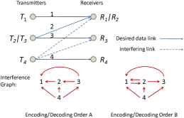
Figure 2: A network with topology loop and encoding/decoding order A is an iTree network, whose interference graph does not have any directional loop. With encoding/decoding order B, it is not an iTree network because the interference graph has directional loops.

Definition 5

A B-MAC network with a fixed coupling matrix is called an Interference Tree (iTree) Network if after interference cancellation, the links can be indexed such that any link is not interfered by the links with smaller indices.

Definition 6

In an Interference Graph, each node represents a link. A directional edge from node $i$ to node $j$ means that link $i$ causes interference to link $j$.

Remark 3

The iTree network is related to but different from the network with tree topology, which implies iTree network only if the interference cancellation order is chosen properly. For example, a MAC which has tree topology is not an iTree network if the successive decoding is not employed at the receiver. On the other hand, even if there are loops in a network, it may be an iTree network if the interference cancellation order is right. We give such an example in Fig. 2 where there are four desired data links 1, 2, 3, and 4, and dirty paper coding and successive decoding and cancellation are employed. With encoding/decoding order A, where the signal $\mathbf{x}_{2}$ is decoded after $\mathbf{x}_{1}$ and the signal $\mathbf{x}_{3}$ is encoded after $\mathbf{x}_{2}$, each link $l\in\left\{2,3,4\right\}$ is not interfered by the first $l-1$ links. Therefore, the network in Fig. 2 is an iTree network even though it has a loop of nonzero channel gains. However, for encoding/decoding order B, SIC is not employed at $R_{1}/R_{2}$, and $\mathbf{x}_{2}$ is encoded after $\mathbf{x}_{3}$ at $T_{2}/T_{3}$. The network in Fig. 2 is no longer an iTree network because the interference graph has directional loops, making the iTree indexing impossible.

Since the coupling matrix of the reverse links is the transpose of that of the forward links, the interference relation is reversed as stated in the following lemmas. Without loss of generality, we consider iTree networks where the $l^{th}$ link is not interfered by the first $l-1$ links in this paper.

Lemma 3

[1] If in an iTree network, the $l^{th}$ link is not interfered by the links with lower indices, in the reverse links, the $l^{th}$ link is not interfered by the links with higher indices.

We develop an algorithm to improve the performance of iTree networks. That is after the convergence of the Algorithm A or B, if any output of the algorithm $\bar{\mathbf{\Sigma}}_{i}$ does not satisfy the polite water-filling structure, the objective (cost) in FOP (SPMP) can be strictly increased (decreased) by enforcing this structure at link $i$.

We first define some notations and give a useful lemma. The output of the SINR based algorithm $\mathbf{\bar{\Sigma}}_{1:L}$ achieves a rate point $\left[\mathcal{I}_{l}\right]_{l=1,...,L}$ with sum power $P_{T}\triangleq\sum_{l=1}^{L}\textrm{Tr}\left(\mathbf{\bar{\Sigma}}_{l}\right)$. The algorithm also produces the corresponding covariance transformation $\bar{\mathbf{\hat{\mathbf{\Sigma}}}}_{1:L}$ computed from $\mathbf{\bar{R}}$ and $\mathbf{\bar{q}}$ achieving a set of rates $\hat{\mathcal{I}}_{l}=\mathcal{I}_{l},l=1,...,L$. Fixing the input covariance matrices $\bar{\mathbf{\Sigma}}_{j},j=i+1,...,L$ for the last $L-i$ links, the first $i$ links form a sub-network

$$\left(\left[\mathbf{H}_{l,k}\right]_{k,l=1,...,i},\sum_{l=1}^{i}\textrm{Tr}\left(\mathbf{\Sigma}_{l}\right)=P_{T}^{i},\left[\mathbf{W}_{l}\right]_{l=1,...i}\right),$$ (39)

where $\mathbf{W}_{l}=\mathbf{I}+\sum_{j=i+1}^{L}\mathbf{\Phi}_{l,j}\mathbf{H}_{l,j}\mathbf{\bar{\Sigma}}_{j}\mathbf{H}_{l,j}^{\dagger},\forall l$ is the covariance matrix of the equivalent colored noise; $P_{T}^{i}=\sum_{l=1}^{i}\textrm{Tr}\left(\mathbf{\bar{\Sigma}}_{l}\right)$. By Theorem 1, the dual sub-network is

$$\left(\left[\mathbf{H}_{k,l}^{\dagger}\right]_{k,l=1,...,i},\sum_{l=1}^{i}\textrm{Tr}\left(\hat{\mathbf{\Sigma}}_{l}\mathbf{W}_{l}\right)=P_{T}^{i},\left[\mathbf{I}_{l}\right]_{l=1,...,i}\right).$$ (40)

It is clear that after convergence, $\bar{\mathbf{\hat{\mathbf{\Sigma}}}}_{1:L}=\left(\mathbf{\bar{\hat{\Sigma}}}_{1},...,\mathbf{\bar{\hat{\Sigma}}}_{L}\right)$ is the covariance transformation of $\mathbf{\bar{\Sigma}}_{1:L}=\left(\mathbf{\bar{\Sigma}}_{1},...,\mathbf{\bar{\Sigma}}_{L}\right)$. By Lemma 9 in [1], $\bar{\hat{\mathbf{\Sigma}}}_{1:i}=\left(\mathbf{\bar{\hat{\Sigma}}}_{1},...,\mathbf{\bar{\hat{\Sigma}}}_{i}\right)$ is also the covariance transformation of $\mathbf{\bar{\Sigma}}_{1:i}=\left(\mathbf{\bar{\Sigma}}_{1},...,\mathbf{\bar{\Sigma}}_{i}\right)$, applied to the sub-network (39).

The algorithm to improve the performance contains three steps.

Step 1: Improve the rate of reverse link $i$ by enforcing the polite water-filling structure on $\hat{\mathbf{\Sigma}}_{i}$. By Lemma 3, the reverse link $i$ causes no interference to the first $i-1$ reverse links. If we fix $\bar{\hat{\mathbf{\Sigma}}}_{l},l=1,...,i-1$, the rate of reverse link $i$ can be improved without hurting other reverse links in the sub network by solving the following single-user optimization problem:

$$\underset{\hat{\mathbf{\Sigma}}_{i}\geq 0}{\textrm{max}}\>\textrm{log}\left|\mathbf{I}+\mathbf{H}_{i,i}^{\dagger}\hat{\mathbf{\Sigma}}_{i}\mathbf{H}_{i,i}\bar{\mathbf{\hat{\mathbf{\Omega}}}}_{i}^{-1}\right|$$ (41)

s.t. $$\>\textrm{Tr}\left(\hat{\mathbf{\Sigma}}_{i}\mathbf{W}_{i}\right)\leq P_{T}^{i}-\sum_{l=1}^{i-1}\textrm{Tr}\left(\bar{\hat{\mathbf{\Sigma}}}_{l}\mathbf{W}_{l}\right)=\textrm{Tr}\left(\bar{\hat{\mathbf{\Sigma}}}_{i}\mathbf{W}_{i}\right),$$

where $\bar{\mathbf{\hat{\mathbf{\Omega}}}}_{i}=\mathbf{I}+\sum_{k=1}^{i-1}\mathbf{\Phi}_{k,i}\mathbf{H}_{k,i}^{\dagger}\mathbf{\bar{\hat{\mathbf{\Sigma}}}}_{k}\mathbf{H}_{k,i}$ and $\mathbf{W}_{i}=\mathbf{I}+\sum_{j=i+1}^{L}\mathbf{\Phi}_{i,j}\mathbf{H}_{i,j}\mathbf{\bar{\Sigma}}_{j}\mathbf{H}_{i,j}^{\dagger}=\bar{\mathbf{\Omega}}_{i}$. By a simple extension of the solution with white noise and sum power constraint in [30] to case of colored noise and linear constraint here, it can be proved that the optimal solution is uniquely given by the following polite water-filling procedure. Perform the thin SVD $\bar{\mathbf{\Omega}}_{i}^{-1/2}\mathbf{H}_{i,i}\bar{\mathbf{\hat{\mathbf{\Omega}}}}_{i}^{-1/2}=\mathbf{F}_{i}\mathbf{\Delta}_{i}\mathbf{G}_{i}^{\dagger}$. Let $N_{i}=\textrm{Rank}\left(\mathbf{H}_{i,i}\right)$ and $\delta_{i,j}$ be the $j^{th}$ diagonal element of $\mathbf{\Delta}_{i}^{2}$. Obtain $\mathbf{D}_{i}$ as

$$\mathbf{D}_{i} = \textrm{diag}\left(d_{i,j},...,d_{i,N_{i}}\right),$$ (42)

$$d_{i,j} = \left(\nu_{i}-\frac{1}{\delta_{i,j}}\right)^{+},j=1,...,N_{i},$$

where $\nu_{i}$ is chosen such that $\sum_{j=1}^{N_{l}}d_{i,j}=\textrm{Tr}\left(\bar{\hat{\mathbf{\Sigma}}}_{i}\bar{\mathbf{\Omega}}_{i}\right)$ and can be obtained by conventional water-filling algorithm. Then the optimal solution is given by

$$\hat{\mathbf{\Sigma}}_{i}^{{}^{\prime}}=\bar{\mathbf{\Omega}}_{i}^{-1/2}\mathbf{F}_{i}\mathbf{D}_{i}\mathbf{F}_{i}^{\dagger}\bar{\mathbf{\Omega}}_{i}^{-1/2}$$ (43)

By Theorem 3, if $\mathbf{\bar{\Sigma}}_{i}$ does not satisfy the polite water-filling, nor does $\bar{\hat{\mathbf{\Sigma}}}_{i}$, which implies that $\bar{\hat{\mathbf{\Sigma}}}_{i}$ is not the optimal solution and $\hat{\mathbf{\Sigma}}_{i}^{{}^{\prime}}$ achieves a rate $\hat{\mathcal{I}}_{i}^{{}^{\prime}}>\hat{\mathcal{I}}_{i}$.

Step 2: Improve the forward links by the covariance transformation from $\mathbf{\hat{\Sigma}}_{1:i}^{{}^{\prime}}=\left(\bar{\hat{\mathbf{\Sigma}}}_{1},...,\bar{\hat{\mathbf{\Sigma}}}_{i-1},\hat{\mathbf{\Sigma}}_{i}^{{}^{\prime}}\right)$ to $\mathbf{\Sigma}_{1:i}^{{}^{\prime}}=\left(\mathbf{\Sigma}_{1}^{{}^{\prime}},...,\mathbf{\Sigma}_{i}^{{}^{\prime}}\right)$ for the sub-network. Due to the special interference structure of iTree networks, the calculation of the transmit powers of the covariance transformation can be simplified to be calculated one by one as follows. When calculating $p_{l,m}$, the transmit powers $p_{k,m}:\ m=1,...,M_{k},\ k=l+1,...i$ and $p_{l,n},\ n=m+1,...,M_{l}$ have been calculated. Therefore, we can calculate $\mathbf{\Sigma}_{k}^{{}^{\prime}}=\sum_{m=1}^{M_{k}}p_{k,m}\mathbf{t}_{k,m}\mathbf{t}_{k,m}^{\dagger},\ k=l+1,...i$ and obtain the interference-plus-noise covariance matrix of the link $l$ as $\mathbf{\Omega}_{l}^{{}^{\prime}}=\mathbf{I}+\sum_{k=l+1}^{i}\mathbf{\Phi}_{l,k}\mathbf{H}_{l,k}\mathbf{\Sigma}_{k}^{{}^{\prime}}\mathbf{H}_{l,k}^{\dagger}$. Then obtain $p_{l,m}$ as

$$p_{l,m}=\frac{\hat{\gamma}_{l,m}\left(\mathbf{r}_{l,m}^{\dagger}\mathbf{\Omega}_{l}^{{}^{\prime}}\mathbf{r}_{l,m}+\sum_{n=m+1}^{M_{l}}p_{l,n}\left|\mathbf{r}_{l,m}^{\dagger}\mathbf{H}_{l,l}\mathbf{t}_{l,n}\right|^{2}\right)}{\left|\mathbf{r}_{l,m}^{\dagger}\mathbf{H}_{l,l}\mathbf{t}_{l,m}\right|^{2}}.$$ (44)

Finally $\mathbf{\Sigma}_{l}^{{}^{\prime}}$ is given by

$$\mathbf{\Sigma}_{l}^{{}^{\prime}} = \sum_{m=1}^{M_{l}}p_{l,m}\mathbf{t}_{l,m}\mathbf{t}_{l,m}^{\dagger}.$$ (45)

By Theorem 1, the covariance transformation $\mathbf{\Sigma}_{1:i}^{{}^{\prime}}$ achieves a set of rates $\mathcal{I}_{i}^{{}^{\prime}}\geq\hat{\mathcal{I}}_{i}^{{}^{\prime}}>\mathcal{I}_{i}$ and $\mathcal{I}_{l}^{{}^{\prime}}\geq\hat{\mathcal{I}}_{l}^{{}^{\prime}}=\mathcal{I}_{l},l<i$ in the sub-network under the sum power constraint $\sum_{l=1}^{i}\textrm{Tr}\left(\mathbf{\Sigma}_{l}^{{}^{\prime}}\right)=\sum_{l=1}^{i-1}\textrm{Tr}\left(\bar{\hat{\mathbf{\Sigma}}}_{l}\mathbf{W}_{l}\right)+\textrm{Tr}\left(\hat{\mathbf{\Sigma}}_{i}^{{}^{\prime}}\mathbf{W}_{i}\right)=P_{T}^{i}$. Noting that the first $i$ links cause no interference to all other links in the original network, the input covariance matrices $\mathbf{\Sigma}_{1:L}^{{}^{\prime}}=\left(\mathbf{\Sigma}_{1}^{{}^{\prime}},\cdots,\mathbf{\Sigma}_{i}^{{}^{\prime}},\mathbf{\bar{\Sigma}}_{i+1},\cdots,\mathbf{\bar{\Sigma}}_{L}\right)$ must achieve a rate point $\mathcal{I}_{i}^{{}^{\prime}}>\mathcal{I}_{i}$ and $\mathcal{I}_{l}^{{}^{\prime}}\geq\mathcal{I}_{l},\forall l\neq i$ in the original network with the same sum power $P_{T}$.

We refer to the above algorithm as Algorithm S and summarize it in table IV.

Table IV: Algorithm S (Improving the Rate of Link $i$ for iTree Networks)

1. Obtain $\bar{\mathbf{\hat{\mathbf{\Sigma}}}}_{1:i}$ from the solution of Algorithm A or B.

2. Solve for the optimal $\mathbf{\hat{\mathbf{\Sigma}}}_{i}^{{}^{\prime}}$ in the optimization problem (41)

by polite water-filling.

3. Calculate the input covariance matrices $\mathbf{\Sigma}_{l}^{{}^{\prime}},l=1,...,i$ for the first

$i$ links by the covariance transformation as in (45).

4. Output the updated input covariance matrices

$\mathbf{\Sigma}_{1:L}^{{}^{\prime}}=\left(\mathbf{\Sigma}_{1}^{{}^{\prime}},\cdots,\mathbf{\Sigma}_{i}^{{}^{\prime}},\mathbf{\bar{\Sigma}}_{i+1},\cdots,\mathbf{\bar{\Sigma}}_{L}\right).$

The performance can be strictly improved using the output of Algorithm S. For FOP, we first reduce the transmit power of link $i$ until its rate is reduced to $\mathcal{I}_{i}$. This may benefit other links as well because the interference to other links is also reduced. Then this extra power can be used to simultaneously increase all link’s power by the same factor, and thus improve the rates of all links and the objective function of FOP. The cost function of SPMP can be strictly decreased by reducing the transmit power of link $i$ such that the rate is reduced to $\mathcal{I}_{i}^{0}$. Note that the above operations can be automatically achieved by Algorithm A (B) using $\mathbf{\Sigma}_{1:L}^{{}^{\prime}}$ as the initial point. According to the above, we propose an improved algorithm for iTree networks using Algorithm S as a component. It is referred to as Algorithm I and summarized in table V. The optimality of Algorithm I is stated in the theorem below.

Table V: Algorithm I (Improved Algorithm for iTree Networks)

1. Generate random initial point such that all streams have

positive SINR.

2. Run Algorithm A or B to obtain the solution $\bar{\mathbf{\Sigma}}_{1:L}$.

3. Repeat

For $i=1:L$

If $\bar{\mathbf{\Sigma}}_{i}$ does not satisfy the polite water-filling structure

Obtain $\mathbf{\Sigma}_{1:L}^{{}^{\prime}}$ from $\bar{\mathbf{\Sigma}}_{1:L}$ using Algorithm S.

Run Algorithm A or B with $\mathbf{\Sigma}_{1:L}^{{}^{\prime}}$ as the initial point to

obtain the solution $\bar{\mathbf{\Sigma}}_{1:L}$.

End

End

Until converge

Theorem 10

For iTree networks, the solution of Algorithm I satisfies all the optimality conditions in Theorem 8, and thus achieves a stationary point.

Proof:

For iTree networks, the SPMP is always feasible. Step 2 of the Algorithm I generates a feasible solution $\bar{\mathbf{\Sigma}}_{1:L}$. Then in step 3, both Algorithm S and Algorithm A (B) will monotonically increase (decrease) the objective (cost) in FOP (SPMP). Since the objective (cost) is upper bounded (lower bounded), Algorithm I must converge to a fixed point. If the optimality conditions in Theorem 8 is not satisfied, Algorithm I will strictly increase (decrease) the objective (cost) in FOP (SPMP), which contradicts with the assumption of fixed point. ∎

Actually, in almost all simulations we conducted for general B-MAC networks, Algorithm A or B with initial point randomly generated from a continuous space is observed to converge to a stationary point. Therefore, Algorithm I seldomly runs Algorithm S. Therefore, Algorithm S is more of theoretic value for the convergence to a stationary point and serve as a basis for the algorithm in the next subsection.

IV-E Polite Water-filling based Algorithms for SPMP

IV-E1 Algorithm PR for iTree Networks

In stead of converting the rate constrained problem to the SINR constrained problem, we can modify Algorithm S to directly solve SPMP for iTree networks. In (42), the polite water-filling level $\nu_{i}$ is chosen such that the sum power is unchanged when switching to the forward links. Because this polite water-filling level will improve the rate of reverse link $i$, if the initial solution is feasible, i.e., the rate of reverse link $i$ is no less than $\mathcal{I}_{i}^{0}$, we can reduce the polite water-filling level $\nu_{i}$ to make the rate of reverse link $i$ equal to $\mathcal{I}_{i}^{0}$, and thus reduce the sum power when switching to the forward links. This results in an algorithm which monotonically decreases the sum power once the solution becomes feasible. A simple algorithm in Table VI referred to as Algorithm W can be used to calculate the polite water-filling level $\nu_{i}$ to satisfy the rate constraint $\mathcal{I}_{i}^{0}$.

Table VI: Algorithm W (Solving the Polite Water-filling Level for the Rate Constraints)

1. Initialize the set of indices of the streams of link $i$ as

$\Gamma=\left\{1,...,N_{i}\right\}$, where $N_{i}=\textrm{Rank}\left(\mathbf{H}_{i,i}\right)$.

2. Calculate $\nu_{i}=\left(e^{\mathcal{I}_{i}^{0}}/\Pi_{j\in\Gamma}\delta_{i,j}\right)^{1/\left|\Gamma\right|}$, which is the solution of

$\sum_{j\in\Gamma}\textrm{log}\left(1+\left(\nu_{i}-1/\delta_{i,j}\right)\delta_{i,j}\right)=\mathcal{I}_{i}^{0}$.

Obtain $d_{i,j}=\nu_{i}-1/\delta_{i,j}$ for $j\in\Gamma$.

3. If $d_{i,j}\geq 0$, $\forall j\in\Gamma$, stop. Otherwise, for all $j\in\Gamma$, if $d_{i,j}<0$,

fix it as $d_{i,j}=0$, delete $j$ from $\Gamma$. Repeat step 2).

This modification of Algorithm S is referred to as Algorithm PR and is summarized in table VII, where P stands for Polite and R stands for Rate constraint. It can be shown that once Algorithm PR finds a feasible solution, it will monotonically decrease the sum power until it converges to a stationary point.

Table VII: Algorithm PR (Solving SPMP for iTree Networks)

Initialize $\mathbf{\Sigma}_{1:L}$ such that $\mathbf{\Sigma}_{i}\succeq 0,\forall i$.

While not converge do

For $i=1:L$

1. Calculate $\hat{\mathbf{\Sigma}}_{1:i}$ by the covariance transformation of $\mathbf{\Sigma}_{1:i}$

applied to the $i^{\text{th}}$ sub-network.

2. Obtain $\mathbf{\hat{\mathbf{\Sigma}}}_{i}^{{}^{\prime}}$ by polite water-filling as in (42) and (43), where

the polite water-filling level $\nu_{i}$ is calculated by Algorithm W.

3. Calculate $\mathbf{\Sigma}_{1:i}^{{}^{\prime}}$ by the covariance transformation of

$\mathbf{\hat{\mathbf{\Sigma}}}_{1:i}^{{}^{\prime}}=\left(\mathbf{\hat{\Sigma}}_{1},...,\mathbf{\hat{\Sigma}}_{i-1},\mathbf{\hat{\Sigma}}_{i}^{{}^{\prime}}\right)$ applied to the $i^{\text{th}}$ sub-network.

4. Update $\mathbf{\Sigma}_{1:L}$ as $\mathbf{\Sigma}_{1:L}=\left(\mathbf{\Sigma}_{1}^{{}^{\prime}},...,\mathbf{\Sigma}_{i}^{{}^{\prime}},\mathbf{\Sigma}_{i+1},...,\mathbf{\Sigma}_{L}\right)$.

End

End

IV-E2 Algorithm PR1 for B-MAC Networks

To get rid of the covariance transformation which is more complex than the polite water-filling as will be discussed later, and to make the algorithm work for general B-MAC networks, we obtain an intuitive algorithm by imposing the polite water-filling structure iteratively. It is referred to as Algorithm PR1 and is summarized in table VIII. It turns out that the algorithm can also be derived from the Lagrange function and KKT conditions of the problem, where the Lagrange multipliers are exactly the water-filling levels of the links. Adjusting the Lagrange multipliers to satisfy the rate constraints is exactly what Algorithm W does. It is clear that if the algorithm converges, the solution of Algorithm PR1 satisfies the optimality conditions in Theorem 8, and thus achieves a stationary point.

Table VIII: Algorithm PR1 (Solving SPMP for B-MAC Networks)

Initialize $\mathbf{\hat{\Sigma}}_{1:L}$ and $\mathbf{\Omega}_{i}$’s such that $\mathbf{\hat{\Sigma}}_{i}\succeq 0,\forall i$ and $\mathbf{\Omega}_{i}=\mathbf{I},\forall i$.

While not converge do

1. Update in the forward links

a. For $\forall i$, obtain $\hat{\mathbf{\Omega}}_{i}$ from $\hat{\mathbf{\Sigma}}_{1:L}$ using (6).

Perform thin SVD $\mathbf{\Omega}_{i}^{-1/2}\mathbf{H}_{i,i}\hat{\mathbf{\Omega}}_{i}^{-1/2}=\mathbf{F}_{i}\mathbf{\Delta}_{i}\mathbf{G}_{i}^{\dagger}$.

b. Obtain $\mathbf{D}_{i}$ by the water-filling in (42), where

the polite water-filling level $\nu_{i}$ is calculated by Algorithm W.

c. Update $\mathbf{\Sigma}_{i}$’s as

$\mathbf{\Sigma}_{i}=\hat{\mathbf{\Omega}}_{i}^{-1/2}\mathbf{G}_{i}\mathbf{D}_{i}\mathbf{G}_{i}^{\dagger}\hat{\mathbf{\Omega}}_{i}^{-1/2},\forall i$.

2. Update in the reverse links

a. For $\forall i$, obtain $\mathbf{\Omega}_{i}$ from $\mathbf{\Sigma}_{1:L}$ using (2).

Perform thin SVD $\mathbf{\Omega}_{i}^{-1/2}\mathbf{H}_{i,i}\hat{\mathbf{\Omega}}_{i}^{-1/2}=\mathbf{F}_{i}\mathbf{\Delta}_{i}\mathbf{G}_{i}^{\dagger}$.

b. Obtain $\mathbf{D}_{i}$ by the water-filling in (42), where

the polite water-filling level $\nu_{i}$ is calculated by Algorithm W.

c. Update $\mathbf{\hat{\Sigma}}_{i}$’s as

$\mathbf{\hat{\Sigma}}_{i}=\mathbf{\Omega}_{i}^{-1/2}\mathbf{F}_{i}\mathbf{D}_{i}\mathbf{F}_{i}^{\dagger}\mathbf{\Omega}_{i}^{-1/2},\forall i$.

End

It is difficult to prove the convergence of Algorithm PR1. But the intuition and all simulations we conducted strongly indicate fast convergence.

Remark 4

Algorithm PR1 can be used to solve the FOP by replacing constraints $\mathcal{I}_{l}^{0}$ with $\alpha\mathcal{I}_{l}^{0}$ and searching for $\alpha$ to satisfy the power constraint.

Remark 5

An advantage of Algorithm PR1 is that it can be easily implemented distributedly as will be shown in Section IV-F. Another advantage is that it has linear complexity in each iteration, because the SVD for polite water-filling is performed over the matrices whose dimensions are not increased with the number of desired data links $L$. However, the complexity order of Algorithm B depends on $L$. In each iteration, the complexity of calculating all the MMSE-SIC receive vectors is still linear with respect to $L$. But to calculate the transmit powers $\mathbf{p}$ and $\mathbf{q}$, we need to solve two $\sum_{l=1}^{L}M_{l}$-dimensional linear equations, whose complexity depends on the density and structure of the cross-talk matrix $\mathbf{\Psi}\left(\mathbf{T},\mathbf{R}\right)$. In the worst case, the complexity order is $\mathcal{O}\left(L^{3}\right)$. In other cases such as with triangular or sparse $\mathbf{\Psi}\left(\mathbf{T},\mathbf{R}\right)$, the complexity is much lower. Fortunately, in practice, $\mathbf{\Psi}\left(\mathbf{T},\mathbf{R}\right)$ is usually sparse for a large wireless network because of path loss.

IV-F Distributed Implementation of Algorithm PR1

In a network, it is desirable to use distributed optimization. The above centralized algorithms serve as the basis for distributed design. Here, we design a distributed algorithm based on Algorithm PR1 for time division duplex (TDD) networks.. To perform the polite water-filling in Algorithm PR1, $T_{l}$ ($R_{l}$) only needs to know the equivalent channel $\mathbf{\Omega}_{l}^{-1/2}\mathbf{H}_{l,l}\hat{\mathbf{\Omega}}_{l}^{-1/2}$, where both $\mathbf{\hat{\Omega}}_{l}$ ($\mathbf{\Omega}_{l}$) and $\mathbf{H}_{l,l}^{\dagger}\mathbf{\Omega}_{l}^{-1/2}$ ($\mathbf{H}_{l,l}\hat{\mathbf{\Omega}}_{l}^{-1/2}$) can be obtained by pilot-aided estimation in the reverse (forward) links in time division duplex (TDD) networks. In frequency division duplex (FDD) networks, the equivalent channel needs to be calculated from feedback. Thus, TDD system has an advantage.

We assume block fading channel, where each block consists of a training stage followed by a transmission stage. The training stage is further divided into several rounds, where one round consists of a half round of pilot aided estimation of $\mathbf{H}_{l,l}\hat{\mathbf{\Omega}}_{l}^{-1/2}$ and $\mathbf{\Omega}_{l}$ in the forward link and a half round of pilot aided estimation of $\mathbf{H}_{l,l}^{\dagger}\mathbf{\Omega}_{l}^{-1/2}$ and $\mathbf{\hat{\Omega}}_{l}$ in the reverse link. Since Algorithm PR1 achieves most of the benefit in very few iterations, the required number of training rounds is small and can be as less as 2.5 rounds. In the training stage, the $T_{l}$’s and $R_{l}$’s run a distributed version of Algorithm PR1 to solve SPMP. At the end of the training stage, $T_{l}$’s use the latest $\mathbf{\Sigma}_{l}$’s as the input covariance matrices for the transmission stage.

First, we describe the operation at each node.

Operation at $T_{l}$:

• In the $\left(i-1\right)^{\text{th}}$ reverse training round, $T_{l}$ estimates the interference-plus-noise covariance matrix $\mathbf{\hat{\Omega}}_{l}^{(i-1)}$ and the effective channel $\mathbf{H}_{l,l}^{\dagger}\left(\mathbf{\Omega}_{l}^{(i-1)}\right)^{-1/2}$.

• At the beginning of the $i^{\text{th}}$ forward training round, $T_{l}$ calculates the input covariance matrix $\mathbf{\Sigma}_{l}^{(i)}$ by polite water-filling over the equivalent channel $\left(\mathbf{\Omega}_{l}^{(i-1)}\right)^{-1/2}\mathbf{H}_{l,l}\left(\mathbf{\hat{\Omega}}_{l}^{(i-1)}\right)^{-1/2}$ as in step 1 of Algorithm PR1. However, in practice, the transmit power of $T_{l}$ can not exceed certain maximum value denoted by $P_{T_{l}}^{\textrm{max}}$. If $\textrm{Tr}\left(\mathbf{\Sigma}_{l}^{(i)}\right)>P_{T_{l}}^{\textrm{max}}$, decrease the polite water-filling level $\nu_{l}$ obtained by Algorithm W until $\textrm{Tr}\left(\mathbf{\Sigma}_{l}^{(i)}\right)=P_{T_{l}}^{\textrm{max}}$. Then $T_{l}$ transmits pilot signals in the $i^{\text{th}}$ forward training round.

Operation at $R_{l}$:

• In the $i^{\text{th}}$ forward training round, $R_{l}$ estimates $\mathbf{\Omega}_{l}^{(i)}$ and $\mathbf{H}_{l,l}\left(\mathbf{\hat{\Omega}}_{l}^{(i-1)}\right)^{-1/2}$.

• At the beginning of the $i^{th}$ reverse training round, $R_{l}$ calculates $\hat{\mathbf{\Sigma}}_{l}^{(i)}$ by polite water-filling over the equivalent channel $\left(\mathbf{\hat{\Omega}}_{l}^{(i-1)}\right)^{-1/2}\mathbf{H}_{l,l}^{\dagger}\left(\mathbf{\Omega}_{l}^{(i)}\right)^{1/2}$ as in step 2 of Algorithm PR1. Denote $P_{R_{l}}^{\textrm{max}}$ as the maximum transmit power of $R_{l}$. If $\textrm{Tr}\left(\hat{\mathbf{\Sigma}}_{l}^{(i)}\right)>P_{R_{l}}^{\textrm{max}}$, decrease the polite water-filling level $\nu_{l}$ obtained by Algorithm W until $\textrm{Tr}\left(\hat{\mathbf{\Sigma}}_{l}^{(i)}\right)=P_{R_{l}}^{\textrm{max}}$. Then $R_{l}$ transmits pilot signals in the $i^{\text{th}}$ reverse training round.

Then, we summarize this distributed algorithm for calculating the input covariance matrices in Table IX and refer to it as Algorithm PRD.

Table IX: Algorithm PRD (Distributed Version of Algorithm PR1)

Initialize $i=1$ and $\mathbf{\Omega}_{l}^{(0)}=\mathbf{I},\>\mathbf{\hat{\Omega}}_{l}^{(0)}=\mathbf{I},\>\forall l$.

1. In the $i^{\textrm{th}}$ forward training round, $T_{l}$ calculates $\mathbf{\Sigma}_{l}^{(i)}$ by polite

water-filling over $\left(\mathbf{\Omega}_{l}^{(i-1)}\right)^{-1/2}\mathbf{H}_{l,l}\left(\mathbf{\hat{\Omega}}_{l}^{(i-1)}\right)^{-1/2}$ and transmits

pilot signals. (In the $1^{\text{st}}$ round, since the equivalent channel is

unknown, $\mathbf{\Sigma}_{l}^{(1)}$ can be chosen randomly.)

$R_{l}$ estimates $\mathbf{\Omega}_{l}^{(i)}$ and $\mathbf{H}_{l,l}\left(\mathbf{\hat{\Omega}}_{l}^{(i-1)}\right)^{-1/2}$.

2. In the $i^{\textrm{th}}$ reverse training round, $R_{l}$ calculates $\mathbf{\hat{\Sigma}}_{l}^{(i)}$ by polite

water-filling over $\left(\mathbf{\hat{\Omega}}_{l}^{(i-1)}\right)^{-1/2}\mathbf{H}_{l,l}^{\dagger}\left(\mathbf{\Omega}_{l}^{(i)}\right)^{-1/2}$ and transmits

pilot signals. $T_{l}$ estimates $\mathbf{\hat{\Omega}}_{l}^{(i)}$ and $\mathbf{H}_{l,l}^{\dagger}\left(\mathbf{\Omega}_{l}^{(i)}\right)^{-1/2}$.

3. Let $i=i+1$ and enter the next round. Keep updating $\mathbf{\Sigma}_{l}^{(i)}$ and

$\hat{\mathbf{\Sigma}}_{l}^{(i)}$ until the end of the training stage.

Note that one training round is almost the same as one iteration in Algorithm PR1 except that the transmit power of each node is constrained not to exceed a maximum value. Therefore, after convergence, if the transmit power of each node does not exceed its maximum transmit power, Algorithm PRD achieves nearly the same performance as Algorithm PR1. However in practice, it is desirable to allocate as less number of training rounds as possible. Then, Algorithm PRD may not be able to fully converge and thus the target rates may not be satisfied. Fortunately, it is observed in the simulations that Algorithm PRD converges very fast at the first few rounds.

IV-G Optimization of the Encoding and Decoding Order

For the special case of using DPC and SIC to cancel interference, the coupling matrix $\mathbf{\Phi}\left(\pi\right)$ is a function of the encoding and decoding order $\pi$. In this section, we partially characterize the optimal encoding and decoding order $\pi$ and design an algorithm to find a good $\pi$. It is in general a difficult problem because the encoding and decoding orders at the BC transmitters and the MAC receivers need to be solved jointly. However, for each Pseudo BC/Pseudo MAC defined below, the optimal $\pi$ is characterized in Theorem 11.

Definition 7

In a B-MAC network, a sub-network with a single physical transmitter and a set of associated links whose indices forms a set $\mathcal{L}_{\textrm{B}}$ is said to be a Pseudo BC if either all links in $\mathcal{L}_{\textrm{B}}$ completely interfere with a link $k$ or all links in $\mathcal{L}_{\textrm{B}}$ do not interfere with a link $k$, $\forall k\in\mathcal{L}_{\textrm{B}}^{C}$, i.e., the columns with indices in $\mathcal{L}_{\textrm{B}}$ of the coupling matrix $\mathbf{\Phi}$, excluding rows in $\mathcal{L}_{\textrm{B}}$, are the same. A sub-network with a single physical receiver and a set of associated links, whose indices forms a set $\mathcal{L}_{\textrm{M}}$, is said to be a Pseudo MAC if either all links in $\mathcal{L}_{\textrm{M}}$ are completely interfered by a link $k$ or all links in $\mathcal{L}_{\textrm{M}}$ are not interfered by a link $k$, $\forall k\in\mathcal{L}_{\textrm{M}}^{C}$, i.e., the rows with indices in $\mathcal{L}_{\textrm{M}}$ of the coupling matrix $\mathbf{\Phi}$, excluding columns in $\mathcal{L}_{\textrm{M}}$, are the same.

Example 1

In Fig. 1, suppose $\mathbf{x}_{1}$ is encoded after $\mathbf{x}_{2}$ and $\mathbf{x}_{4}$ is the last one to be decoded at the second physical receiver. Then link 2 and link 3 forms a pseudo MAC because they belong to the same physical receiver and suffer the same interference from $\mathbf{x}_{1}$, $\mathbf{x}_{4}$ and $\mathbf{x}_{5}$. Similarly, link 4 and link 5 forms a pseudo BC.

Remark 6

The pseudo BC and pseudo MAC were first introduced in [1] where the optimal encoding/decoding order of each pseudo BC/pseudo MAC for the weighted sum-rate maximization problem (WSRMP) is shown to be consistent with the optimal order of an individual BC or MAC. This is because a Pseudo BC or a Pseudo MAC can be isolated from the B-MAC network to form an individual BC or MAC. Similar results can also be obtained for FOP and SPMP as shown below.

First, we need to modify the FOP and SPMP to include encoding and decoding order optimization and time sharing. Let $\mathbf{\Xi}$ be a set of valid coupling matrices produced by proper encoding and decoding orders of a B-MAC network. Define a larger achievable region

$$\mathcal{R}(P_{T}) = \text{Convex Closure}\bigcup_{\mathbf{\Phi}\in\mathbf{\Xi}}\mathcal{R}_{\mathbf{\Phi}}\left(P_{T}\right).$$

The modified optimization problems are

OFOP: $$\underset{\mathbf{r}\in\mathcal{R}(P_{T})}{\textrm{max}} \left(\min_{1\leq l\leq L}\frac{r_{l}}{\mathcal{I}_{l}^{0}}\right),$$ (46)

and

OSPMP: $$\underset{P_{T}}{\textrm{min}} P_{T}$$

s.t. $$[\mathcal{I}_{l}^{0}]_{l=1,...,L}\in\mathcal{R}(P_{T}).$$

The following lemma is a consequence of that all outer boundary points of $\mathcal{R}(P_{T})$ are Pareto optimal and can be proved by contradiction.

Lemma 4

The optimal solution of OFOP or OSPMP is the intersection of the ray $\alpha\left[\mathcal{I}_{1}^{0},\cdots,\mathcal{I}_{L}^{0}\right],\ \alpha>0$, and the boundary of $\mathcal{R}(P_{T})$, where for OSPMP, the sum power $P_{T}$ is chosen such that the intersection is at $\left[\mathcal{I}_{1}^{0},\cdots,\mathcal{I}_{L}^{0}\right]$.

The following theorem characterizes the optimal encoding and decoding order for those boundary points of $\mathcal{R}(P_{T})$ that can be achieved without time sharing and by DPC and SIC. The sufficiency part only holds for MAC and BC.

Theorem 11

Necessity: If the input covariance matrices $\mathbf{\tilde{\Sigma}}_{1:L}$ and the encoding and decoding order $\tilde{\pi}$ for a valid coupling matrix achieves the optimum of OFOP and OSPMP without time sharing, they must satisfy the following necessary conditions:

1. $\mathbf{\tilde{\Sigma}}_{1:L}$ satisfies the optimality conditions in Theorem 8.

2. If there exists a pseudo BC (pseudo MAC) in the B-MAC network, its optimal encoding (decoding) order $\tilde{\pi}$ satisfies that, the signal of the link with the $n^{\text{th}}$ largest (smallest) polite water-filling level is the $n^{\text{th}}$ one to be encoded (decoded).

Sufficiency: In MAC or BC, if certain $\mathbf{\tilde{\Sigma}}_{1:L}$ and $\tilde{\pi}$ satisfy the above conditions, then $\tilde{\mathbf{\Sigma}}_{1:L}$ and $\tilde{\pi}$ achieves the global optimum of OFOP or OSPMP.

Proof:

The first necessary condition follows from Theorem 8. Then the second necessary condition follows from the following two facts and Lemma 4. 1) Any outer boundary point of $\mathcal{R}(P_{T})$ must be the solution of a WSRMP with certain weight vector $\left[w_{l}\right]_{,l=1,...,L}$. It is proved in [1] that the optimal input covariance matrices maximizing the weighted sum-rate must satisfy the polite water-filling structure and the polite water-filling levels are given by $\nu w_{l}$’s for some constant $\nu>0$; 2) By Theorem 9 in [1], the weighted sum-rate optimal encoding and decoding order of each Pseudo BC (Pseudo MAC) is that the signal of the link with the $n^{\text{th}}$ largest (smallest) weight is the $n^{\text{th}}$ one to be encoded (decoded). For the sufficiency part, suppose certain $\mathbf{\tilde{\Sigma}}_{1:L}$ and $\tilde{\pi}$ satisfy the two conditions in Theorem 11. For MAC, satisfying the second condition implies that the weighted sum rate $\sum_{l}^{L}\tilde{\nu}_{l}\mathcal{I}_{l}\left(\mathbf{\Sigma}_{1:L},\mathbf{\Phi}\left(\pi\right)\right)$ is a concave function of $\mathbf{\Sigma}_{1:L}$, where $\tilde{\nu}_{l}$’s are the polite water-filling levels of $\mathbf{\tilde{\Sigma}}_{1:L}$. Then from the proof for the sufficiency part of Theorem 8, $\mathbf{\tilde{\Sigma}}_{1:L}$ and $\tilde{\pi}$ maximizes the weighted sum-rate $\sum_{l}^{L}\tilde{\nu}_{l}\mathcal{I}_{l}\left(\mathbf{\Sigma}_{1:L},\mathbf{\Phi}\left(\pi\right)\right)$ and thus achieves a boundary point of the capacity region of MAC. By Lemma 4, they achieve the global optimality of OFOP or OSPMP. The sufficiency part for BC follows from the rate duality. ∎

The proof of Theorem 11 suggests an algorithm to improve the encoding/decoding order for each pseudo BC and pseudo MAC by simply updating the encoding and decoding order according to current polite water-filling levels. We refer to it as Algorithm O and summarize it in Table X.

Table X: Algorithm O (Improving the Encoding and Decoding Order)

Initialize the encoding and decoding order $\pi$ such that $\mathbf{\Phi}\left(\pi\right)$ is valid.

1. Solve the FOP or SPMP with fixed $\mathbf{\Phi}\left(\pi\right)$.

2. Calculate the polite water-filling levels from the solution of FOP or

SPMP obtained in step 1.

3. For each Pseudo BC and Pseudo MAC with the polite water-filling

levels obtained in step 2, if $\pi$ satisfies Theorem 11, output $\pi$ and

stop. Otherwise, set $\pi$ to satisfy Theorem 11 and return to step 1.

Remark 7

For the special cases of MAC and BC, if Algorithm O converges, the solution gives the optimal order by Theorem 11.

Remark 8

Optimal and sub-optimal algorithms for the special case of solving OSPMP for SIMO MAC/MISO BC have been proposed in [16]. The optimal algorithm is much more complex than Algorithm O as it involves several inner and outer iterations. The difference between Algorithm O and the sub-optimal algorithm are as follows. 1) The sub-optimal algorithm works for SIMO MAC, avoiding the calculation of beamforming matrices, while Algorithm O works for MIMO cases; 2) To find the encoding/decoding order, after obtain the optimal solution of SPMP with fixed $\pi$ in step 1, the sub-optimal algorithm in [16] needs to solve an equation to obtain a weight vector $\left[w_{l}\right]_{,l=1,...,L}$ such that $\left[\mathcal{I}_{1}^{0},\cdots,\mathcal{I}_{L}^{0}\right]$ is the optimal solution of the WSRMP with the weights $w_{l}$’s and fixed $\pi$, while in Algorithm O, the weight vector is directly given by the polite water-filling levels. Same as the algorithm in [16], it is possible for Algorithm O to cycle through a finite number of orders. In this case, we can simply choose the best one from the finite number of orders. For MAC and BC, it is observed that the reason of non-convergence is that the corresponding boundary point can not be achieved without time-sharing.

Remark 9

Algorithms to solve OFOP and OSPMP for MIMO BC have been proposed in [15] where the problems are converted to the weighted sum-rate maximization problem. The algorithms need to repeatedly solve a weighted sum-rate maximization problem for weight vectors searched by the ellipsoid algorithm. The weighted sum-rate maximization problem is solved by the steepest ascent algorithm. For OSPMP, additional search for the total power is also needed. In contrast, Algorithm O solves the problems directly in one sequence of iterations, replaces the steepest ascent algorithm with SINR based algorithms or polite water-filling, only searches weight vector suggested by the polite water-filling level, resulting in much lower complexity.

Remark 10

For BC and MAC, we can also use a simpler encoding/decoding order in [31] which is shown to be asymptotically optimal for MAC (and thus also for BC by duality) when the target rate of each user is the same and the number of users is large. At each transmitter (receiver), the signal of the link with its channel matrix having the $n^{\text{th}}$ smallest (largest) dominant singular value is the $n^{\text{th}}$ one to be encoded (decoded). For convenience, we refer to this order as MEB (maximum eigenmode beamforming) order. It can be shown that MEB order is optimal for SISO MAC and BC.

V Simulation Results

Simulations are used to verify the performance of the proposed algorithms. Let each transmitter and receiver are equipped with $L_{T}$ and $L_{R}$ antennas respectively. DPC and SIC are employed for interference cancellation. Block fading channel is assumed and the channel matrices are independently generated by $\mathbf{H}_{l,k}=\sqrt{g_{l,k}}\mathbf{H}_{l,k}^{\text{(W)}},\forall k,l$, where $\mathbf{H}_{l,k}^{\text{(W)}}$ has zero-mean i.i.d. Gaussian entries with unit variance; and $g_{l,k},\forall k,l$ is a positive number and the value is set as $0\textrm{dB}$ except for Fig. 5 and Fig. 6. In Fig. 7-9, each simulation is averaged over 100 random channel realizations, while in other figures, a single channel realization is considered. In all simulations we conducted, Algorithm A, B, PR and PR1 are observed to converge to a stationary point of the corresponding problem. We call pseudo global optimum the best solution among many solutions obtained by running the algorithm for many times with different initial points and with the encoding/decoding order obtained by Algorithm O. For the plots with iteration numbers, we show rates or power after $x.5$ iterations/rounds, where the last 0.5 iteration/round is the forward link update.

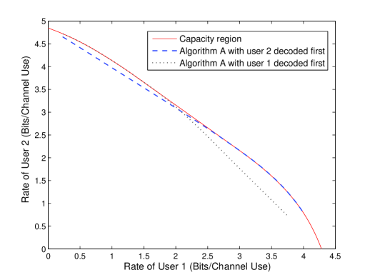
Figure 3: Achieved rate region boundaries of a two-user MAC

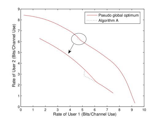
Figure 4: Achieved rate region Boundary of a two-user interference channel

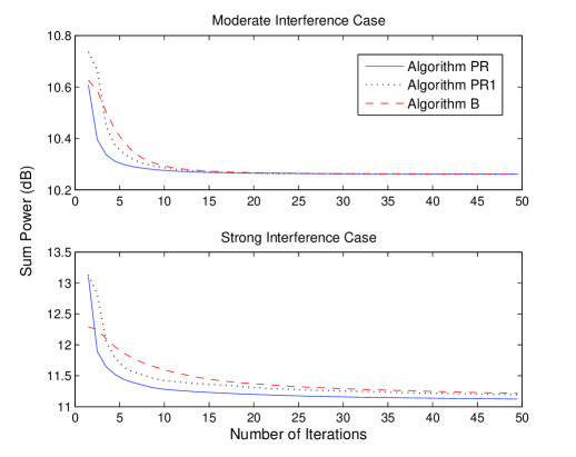
Figure 5: Convergence of the algorithms for the iTree network in Fig. 2

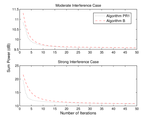
Figure 6: Convergence of the algorithms for a 3-user interference channel

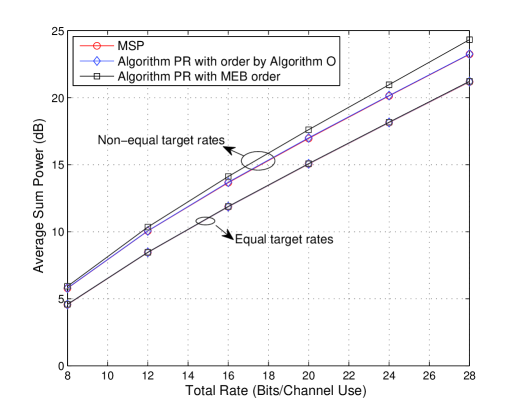
Figure 7: Average sum power vs. the total rate for a 4-user MAC

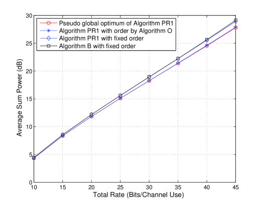
Figure 8: Average sum power vs. the total rate for the B-MAC network in Fig. 1

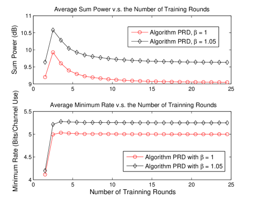
Figure 9: Convergence of the distributed algorithm for a 3-user interference channel

Algorithm A can be used to find the achievable rate region boundary by varying the target rates $\mathcal{I}_{l}^{0}$’s. It finds the point where the boundary is intersected by the ray $\alpha\left(\mathcal{I}_{1}^{0},\cdots,\mathcal{I}_{L}^{0}\right)$. In Fig. 3, we plot the boundaries of the rate regions achieved by Algorithm A with different decoding orders for a two-user MAC with $L_{T}=2,\ L_{R}=4$. It can be observed that the convex hull of the rate regions achieved by Algorithm A is the same as the capacity region, which implies that Algorithm A does achieve the global optimum for this case, and thus is a low complexity approach to calculate the capacity region for MIMO MAC. In Fig. 4, we plot the boundary of the rate region achieved by Algorithm A for a two-user interference channel with $L_{T}=2,\ L_{R}=4$. The pseudo optimum boundary achieved by Algorithm A is also plotted for comparison. In most places, the two boundaries overlap with each other except for a small area. It demonstrates that Algorithm A can find good solutions even with a single initial point.

We demonstrate the superior convergence speed of Algorithm PR and PR1. Sum power versus iteration number is shown in Fig. 5 for the iTree network of Fig. 2 and in Fig. 6 for a 3-user interference channel. Each node has four antennas. The target rate for each link is set as 5 bits/channel use. In the upper sub-plot of Fig. 5, we consider the moderate interference case, where we set $g_{l,k}=0\textrm{dB},\ \forall k,l$. In the lower sub-plot of Fig. 5, we consider strong interference case, where we set $g_{l,3}=10\textrm{dB},\ l=1,2$ for the interfering links, and $g_{l,k}=0\textrm{dB}$ for other $k,l$’s. It is not surprising that Algorithms PR and PR1 have faster convergence speed because polite water-filling exploits the structure of the problem. In the upper sub-plot of Fig. 6, we set $g_{l,k}=0\textrm{dB},\forall k,l$. In the lower sub-plot, we consider a strong interference channel, i.e., $g_{l,k}=10\textrm{dB},\forall k\neq l$, and $g_{l,k}=0\textrm{dB},\forall k=l$. Again, Algorithm PR1 converges faster than Algorithm B. Since the problem is non-convex, the algorithms may converge to different stationary points. But it can be observed that all the stationary points achieve similar performance.

In Fig. 7, we evaluate the performance of Algorithm PR for a 4-user MAC with $L_{T}=2,\ L_{R}=4$. The ‘MSP’ is the optimal solution obtained by the ‘Algorithm 2’ in [15], which has much higher complexity as discussed in Section I-B. For Algorithm PR, both the order obtained by Algorithm O and the MEB order is considered. When the target rate for each user is the same, Algorithm PR with both decoding orders achieves nearly the same sum power as the MSP but with much lower complexity. When the target rates of the users are different and are set as $\left[R_{s},2R_{s},4R_{s},8R_{s}\right]/15$, where $R_{s}$ is the total required rate, Algorithm PR with the order obtained by Algorithm O still achieves near-optimal performance, while Algorithm PR with the MEB order performs worse than that. Not showing is that Algorithm B and PR1 also achieve the same performance as Algorithm PR. In Fig. 8, we evaluate the performance of Algorithms B and PR1 for the B-MAC network in Fig. 1 with $L_{T}=L_{R}=4$. The target rates are set as $\left[R_{s},R_{s},2R_{s},4R_{s},8R_{s}\right]/16$. The encoding/decoding order is partially fixed and is the same as that in Example 1 of Section IV-G. For the pseudo MAC formed by link 2 and link 3 and the pseudo BC formed by link 4 and link 5, the fixed order that $\mathbf{x}_{3}$ is decoded after $\mathbf{x}_{2}$ and $\mathbf{x}_{5}$ is decoded after $\mathbf{x}_{4}$, and its improved order obtained by Algorithm O are applied. With the improved order obtained by Algorithm O, the performance of Algorithm B is not shown because both algorithms achieve nearly the same performance as the Pseudo global optimum of Algorithm PR1, while the algorithms with the fixed order suffers a performance loss.

We illustrate the convergence behavior of the distributed optimization with local CSI. Fig. 9 plots the total transmit power and the minimum rate of the users achieved by Algorithm PRD versus the number of training rounds for a 3-user interference channel with $L_{T}=L_{R}=4$. In Algorithm PRD, the target rates are set as $\beta\left(\mathcal{I}_{1}^{0},\mathcal{I}_{2}^{0},\mathcal{I}_{3}^{0}\right)$ with $\beta=1$ and $\beta=1.05$ respectively, where $\mathcal{I}_{l}^{0}=5$ (bits/channel use), $l=1,2,3$. It can be observed that after 2.5 rounds the rates are close to the targets and after $3.5$ rounds, the powers are also close to the that of infinite rounds. When $\beta=1$, the achieved minimum rate after $3.5$ rounds equals to or exceeds 5 (bits/channel use) in 88 out of 100 simulations. When $\beta=1.05$, achieved minimum rate after $3.5$ rounds equals to or exceeds 5 (bits/channel use) in all 100 simulations, while the total transmit power is about 0.7 dB larger. This suggests a trick that use higher target rates than true targets in order to satisfy the target rates in fewer number of iterations at the expense of more power.

VI Conclusion

The general MIMO one-hop interference networks named B-MAC networks with Gaussian input and any valid coupling matrices are considered. We design algorithms for maximizing the minimum of weighted rates under sum power constraints and for minimizing sum power under rate constraints. They can be used in admission control and in guaranteeing the quality of service. Two kinds of algorithms are designed. The first kind takes advantage of existing SINR optimization algorithms by finding simple and optimal mappings between the achievable rate region and the SINR region. The mappings can be used for many other optimization problems. The second kind takes advantage of the polite water-filling structure of the optimal input found in [1]. Both centralized and distributed algorithms are designed. The proposed algorithms are either proved or shown by simulations to converge to a stationary point, which may not be optimal for non-convex cases, but is shown by simulations to be good solutions.

-A Proof for Theorem 4

Because each link is equivalent to a single-user channel after whitening the interference plus noise, we only need to prove that for any $\mathbf{\Sigma}$ achieving a rate $\mathcal{I}\left(\mathbf{\Sigma}\right)=\textrm{log}\left|\mathbf{I}+\mathbf{H\Sigma H^{\dagger}}\right|$ in a single-user channel $\mathbf{H}$, there exists a decomposition of $\mathbf{\Sigma}=\dot{\mathbf{T}}\dot{\mathbf{T}}^{\dagger}$ leading to $\left\{\mathbf{T},\mathbf{R},\mathbf{p}\right\}$ which achieves a set of SINRs $\gamma_{m}=e^{\mathcal{I}\left(\mathbf{\Sigma}\right)/M}-1,m=1,...,M$.

First, we show that considering unitary precoding matrix $\mathbf{V}\in\mathbb{C}^{M\times M}$ will not loss generality. Note that $\mathcal{I}\left(\mathbf{\Sigma}\right)=\textrm{log}\left|\mathbf{I}+\mathbf{H}\dot{\mathbf{T}}\mathbf{VV^{\dagger}}\dot{\mathbf{T}}^{\dagger}\mathbf{H^{\dagger}}\right|=\textrm{log}\left|\mathbf{I}+\mathbf{\bar{H}VV^{\dagger}\bar{H}^{\dagger}}\right|,$ where $\mathbf{\bar{H}}=\mathbf{H}\dot{\mathbf{T}}$ is the equivalent channel with unitary precoding matrix $\mathbf{V}=\left[\mathbf{v}_{1},...,\mathbf{\mathbf{v}}_{M}\right]$. Define

$$\bar{\mathbf{A}}_{m}=\bar{\mathbf{H}}^{\dagger}\left(\sum_{i=m+1}^{M}\mathbf{\bar{H}}\mathbf{v}_{i}\mathbf{v}_{i}^{\dagger}\mathbf{\bar{H}}^{\dagger}+\mathbf{I}\right)^{-1}\mathbf{\bar{H}}.$$

The SINR of the $m^{th}$ stream achieved by the MMSE-SIC receiver is given by [26]

$$\gamma_{m}=\mathbf{v}_{m}^{\dagger}\bar{\mathbf{A}}_{m}\mathbf{v}_{m}.$$

Hence, we only need to find a unitary precoding matrix $\mathbf{V}$ such that $\mathbf{v}_{m}^{\dagger}\bar{\mathbf{A}}_{m}\mathbf{v}_{m}=e^{\mathcal{I}\left(\mathbf{\Sigma}\right)/M}-1,m=1,...,M$. Then the precoding matrix for the original channel is give by $\dot{\mathbf{T}}^{{}^{\prime}}=\dot{\mathbf{T}}\mathbf{V}$.

We will use the method of induction. We first find a unit vector $\mathbf{v}_{M}$ such that $\mathbf{v}_{M}^{\dagger}\bar{\mathbf{A}}_{M}\mathbf{v}_{M}=e^{\mathcal{I}\left(\mathbf{\Sigma}\right)/M}-1$. Let $\lambda_{i}^{(M)}$ be the $i^{th}$ largest eigenvalue of $\bar{\mathbf{A}}_{M}$ and $\mathbf{u}_{i}^{(M)}$ be the corresponding eigenvector. Since $\mathcal{I}\left(\mathbf{\Sigma}\right)=\textrm{log}\left|\mathbf{I}+\mathbf{\bar{H}VV^{\dagger}\bar{H}^{\dagger}}\right|=\textrm{log}\left|\mathbf{I}+\bar{\mathbf{A}}_{M}\right|=\textrm{log}\prod_{i=1}^{M}\left(1+\lambda_{i}^{(M)}\right)$, we must have $\lambda_{1}^{(M)}\geq e^{\mathcal{I}\left(\mathbf{\Sigma}\right)/M}-1$ and $\lambda_{M}^{(M)}\leq e^{\mathcal{I}\left(\mathbf{\Sigma}\right)/M}-1$. Note that $\mathbf{v}_{M}^{\dagger}\bar{\mathbf{A}}_{M}\mathbf{v}_{M}=\sum_{i=1}^{M}\left|\mathbf{v}_{M}^{\dagger}\mathbf{u}_{i}^{(M)}\right|^{2}\lambda_{i}^{(M)}.$ Because $\left\{\mathbf{u}_{i}^{(m)},i=1,...,M\right\}$ form orthogonal bases, there exists a $\mathbf{v}_{M}$ such that

$$\left|\mathbf{v}_{M}^{\dagger}\mathbf{u}_{i}^{(M)}\right|^{2} =0,\ i=2,...,M-1,$$

$$\left|\mathbf{v}_{M}^{\dagger}\mathbf{u}_{1}^{(M)}\right|^{2}\lambda_{1}^{(M)}+ \left|\mathbf{v}_{M}^{\dagger}\mathbf{u}_{1}^{(M)}\right|^{2}\lambda_{M}^{(M)}=e^{\mathcal{I}\left(\mathbf{\Sigma}\right)/M}-1.$$

Then it follows $\mathbf{v}_{M}^{\dagger}\bar{\mathbf{A}}_{M}\mathbf{v}_{M}=e^{\mathcal{I}\left(\mathbf{\Sigma}\right)/M}-1$.

Assume we already found a set of mutual orthogonal unit vectors $\mathbf{v}_{l},l=m+1,...,M$ such that $\mathbf{v}_{l}^{\dagger}\bar{\mathbf{A}}_{l}\mathbf{v}_{l}=e^{\mathcal{I}\left(\mathbf{\Sigma}\right)/M}-1,l=m+1,...,M$. The rest is to prove that there exists a $\mathbf{v}_{m}$ such that $\mathbf{v}_{m}^{\dagger}\bar{\mathbf{A}}_{m}\mathbf{v}_{m}=e^{\mathcal{I}\left(\mathbf{\Sigma}\right)/M}-1$ and $\mathbf{v}_{m}$ is orthogonal to $\mathbf{v}_{l},l=m+1,...,M$. Perform SVD $\bar{\mathbf{A}}_{m}=\mathbf{U}_{m}\mathbf{D}_{m}\mathbf{U}_{m}^{\dagger}$. Let $\lambda_{n}^{(m)}$ be the $n^{th}$ largest eigenvalue of $\bar{\mathbf{A}}_{m}$ and $\mathbf{u}_{n}^{(m)}$ be the corresponding eigenvector. Define $\mathbf{\hat{u}}_{n}^{(m)}=\mathbf{u}_{n}^{(m)}-\sum_{j=m+1}^{M}\mathbf{v}_{j}^{\dagger}\mathbf{u}_{n}^{(m)}\mathbf{v}_{j},n=1,...,M$, $\mathbf{\hat{U}}_{m}=\left[\mathbf{\hat{u}}_{1}^{(m)},...,\mathbf{\hat{u}}_{M}^{(m)}\right]$ and $\mathbf{\tilde{A}}_{m}=\mathbf{\hat{U}}_{m}\mathbf{D}_{m}\mathbf{\hat{U}}_{m}^{\dagger}$. Then for $i,j=1,...,m$, we have

$$\mathbf{v}_{i}^{\dagger}\bar{\mathbf{A}}_{m}\mathbf{v}_{j}= \mathbf{v}_{i}^{\dagger}\sum_{n=1}^{M}\mathbf{u}_{n}^{(m)}\lambda_{n}^{(m)}\left(\mathbf{u}_{n}^{(m)}\right)^{\dagger}\mathbf{v}_{j}$$

$$= \mathbf{v}_{i}^{\dagger}\sum_{n=1}^{M}\mathbf{\hat{u}}_{n}^{(m)}\lambda_{n}^{(m)}\left(\mathbf{\hat{u}}_{n}^{(m)}\right)^{\dagger}\mathbf{v}_{j}$$ (48)

$$= \mathbf{v}_{i}^{\dagger}\mathbf{\tilde{A}}_{m}\mathbf{v}_{j},$$

where (48) follows from the definition of $\mathbf{\hat{u}}_{n}^{(m)}$ and the fact that $\mathbf{v}_{i}^{\dagger}\mathbf{v}_{k}=0,$ $i=1,...,m$, $k=m+1,...,M$. Because $\mathbf{\tilde{A}}_{m}$ is positive semidefinite and

$$\mathbf{\tilde{A}}_{m}\mathbf{v}_{i}=\mathbf{0},i=m+1,...,M,$$ (49)

the rank of $\mathbf{\tilde{A}}_{m}$ must be less than $m+1$. Let $\tilde{\lambda}_{i}^{(m)}$ be the $i^{th}$ largest eigenvalue of $\mathbf{\tilde{A}}_{m}$ and $\mathbf{\tilde{u}}_{i}^{(m)}$ be the corresponding eigenvector. Then we must have $\tilde{\lambda}_{i}^{(m)}=0,i=m+1,...,M$. Define $\mathbf{V}_{m}=\left[\mathbf{v}_{1},...,\mathbf{\mathbf{v}}_{m}\right]$. Note that the interference from the last $M-m$ streams is $\sum_{i=m+1}^{M}\mathbf{\bar{H}}\mathbf{v}_{i}$ . Then the sum rate of the first $m$ streams is given by

$$\textrm{log}\left|\mathbf{I}+\mathbf{\bar{H}}\mathbf{V}_{m}\mathbf{V}_{m}^{\dagger}\mathbf{\bar{H}^{\dagger}}\left(\sum_{i=m+1}^{M}\mathbf{\bar{H}}\mathbf{v}_{i}\mathbf{v}_{i}^{\dagger}\mathbf{\bar{H}}^{\dagger}+\mathbf{I}\right)^{-1}\right|$$

$$= \textrm{log}\left|\mathbf{I}+\mathbf{V}_{m}^{\dagger}\bar{\mathbf{A}}_{m}\mathbf{V}_{m}\right|$$

$$= \textrm{log}\left|\mathbf{I}+\mathbf{V}_{m}^{\dagger}\mathbf{\tilde{A}}_{m}\mathbf{V}_{m}\right|$$ (50)

$$= \textrm{log}\left|\mathbf{I}+\mathbf{V}^{\dagger}\mathbf{\tilde{A}}_{m}\mathbf{V}\right|$$ (51)

$$= \textrm{log}\prod_{i=1}^{m}\left(1+\tilde{\lambda}_{i}^{(m)}\right)=\frac{m}{M}\mathcal{I}\left(\mathbf{\Sigma}\right),$$

where (50) and (51) follows from (48) and (49) respectively. Therefore we must have $\tilde{\lambda}_{1}^{(m)}\geq e^{\mathcal{I}\left(\mathbf{\Sigma}\right)/M}-1$ and $\tilde{\lambda}_{m}^{(m)}\leq e^{\mathcal{I}\left(\mathbf{\Sigma}\right)/M}-1$. Note that

$$\mathbf{v}_{m}^{\dagger}\bar{\mathbf{A}}_{m}\mathbf{v}_{m} =\mathbf{v}_{m}^{\dagger}\mathbf{\tilde{A}}_{m}\mathbf{v}_{m}$$

$$=\sum_{n=1}^{M}\left|\mathbf{v}_{m}^{\dagger}\mathbf{\tilde{u}}_{n}^{(m)}\right|^{2}\tilde{\lambda}_{n}^{(m)}.$$

Because $\left\{\mathbf{\tilde{u}}_{i}^{(m)},i=1,...,m\right\}$ form orthogonal bases of the $m$-dimensional subspace orthogonal to $\mathbf{v}_{l},l=m+1,...,M$, there exits a unit vector $\mathbf{v}_{m}$ in this subspace such that

$$\left|\mathbf{v}_{m}^{\dagger}\tilde{\mathbf{u}}_{i}^{(m)}\right|^{2} =0,i=2,...,m-1,m+1,...,M,$$

$$\left|\mathbf{v}_{m}^{\dagger}\mathbf{\tilde{u}}_{1}^{(m)}\right|^{2}\tilde{\lambda}_{1}^{(m)}+ \left|\mathbf{v}_{m}^{\dagger}\mathbf{\tilde{u}}_{m}^{(m)}\right|^{2}\tilde{\lambda}_{m}^{(m)}=e^{\mathcal{I}\left(\mathbf{\Sigma}\right)/M}-1.$$

Then we have $\mathbf{v}_{m}^{\dagger}\bar{\mathbf{A}}_{m}\mathbf{v}_{m}=e^{\mathcal{I}\left(\mathbf{\Sigma}\right)/M}-1$. This completes the proof.

-B Proof for Theorem 5

Note that $\mathbf{\Sigma}=\sum_{m=1}^{M}p_{m}\mathbf{t}_{m}\mathbf{t}_{m}^{\dagger}$ implies that $M\geq\text{Rank}(\mathbf{\Sigma})$. Define an $M\times M$ DFT matrix $\mathbf{F}$ where the element at the $k^{th}$ row and $l^{th}$ column is $\mathbf{F}_{k,l}=e^{-\frac{2\pi kl}{M}j}/\sqrt{M}$. If $M$ is chosen to be greater than or equal to $L_{T}$, let $\mathbf{F}_{0}\in\mathbb{C}^{L_{T}\times M}$ be the matrix comprised of the first $L_{T}$ rows of $\mathbf{F}$. Otherwise, let $\mathbf{F}_{0}\in\mathbb{C}^{L_{T}\times M}$ be the matrix such that the upper sub matrix are $\mathbf{F}$, and other elements are zero. Perform SVD $\mathbf{\Sigma}=\mathbf{U}\mathbf{D}\mathbf{U}^{\dagger}$, where the diagonal elements of $\mathbf{D}$ are positive and in descending order. Let $\dot{\mathbf{T}}=\mathbf{U}\mathbf{D}^{1/2}\mathbf{F}_{0}$. It can be verified that $\dot{\mathbf{T}}\dot{\mathbf{T}}^{\dagger}=\mathbf{\Sigma}$. The norms of the columns of $\dot{\mathbf{T}}$ are the diagonal elements of $\dot{\mathbf{T}}^{\dagger}\dot{\mathbf{T}}=\mathbf{F}_{0}^{\dagger}\mathbf{D}\mathbf{F}_{0}$ and they are equal to $\frac{\sum_{i=1}^{L_{T}}\mathbf{D}_{i,i}}{M}$. Then the corresponding transmit powers satisfy $p_{m}=\textrm{Tr}\left(\mathbf{\mathbf{\Sigma}}\right)/M,\forall m$.

-C Proof of the Theorem 8

First, we show that any $\tilde{\mathbf{\Sigma}}_{1:L}$ satisfying the optimality conditions for FOPa must satisfy the KKT conditions of FOPa. The Lagrangian of FOPa (IV-C) is

$$L\left(\mathbf{\Sigma}_{1:L},\nu_{l},\mathbf{\Theta}_{1:L}\right)$$ (52)

$$= \frac{\left(1-\sum_{l\neq 1}\nu_{l}\right)}{\mathcal{I}_{1}^{0}}\mathcal{I}_{1}\left(\mathbf{\Sigma}_{1:L},\mathbf{\Phi}\right)+\frac{\sum_{l\neq 1}\nu_{l}}{\mathcal{I}_{l}^{0}}\mathcal{I}_{l}\left(\mathbf{\Sigma}_{1:L},\mathbf{\Phi}\right)$$

$$+\mu\left(P_{T}-\sum_{l=1}^{L}\textrm{Tr}\left(\mathbf{\Sigma}_{l}\right)\right)+\sum_{l=1}^{L}\textrm{Tr}\left(\mathbf{\Sigma}_{l}\mathbf{\Theta}_{l}\right).$$

The KKT conditions are

$$\nabla_{\mathbf{\Sigma}_{l}}L=0,\ \textrm{Tr}\left(\mathbf{\Sigma}_{l}\mathbf{\Theta}_{l}\right)=0,\ \mathbf{\Sigma}_{l},\mathbf{\Theta}_{l}\succeq 0,\ \forall l;$$

$$\nu_{l}\geq 0,\ \mathcal{I}_{1}^{0}\mathcal{I}_{l}\left(\mathbf{\Sigma}_{1:L},\mathbf{\Phi}\right)=\mathcal{I}_{l}^{0}\mathcal{I}_{1}\left(\mathbf{\Sigma}_{1:L},\mathbf{\Phi}\right),\ \forall l\neq 1;$$ (53)

$$\mu\geq 0,\ P_{T}=\sum_{l=1}^{L}\textrm{Tr}\left(\mathbf{\Sigma}_{l}\right).$$

Recall $\tilde{\nu}_{l}$ is the polite water-filling level in the optimality condition. Let $\mu=1/\sum_{l=1}^{L}\mathcal{I}_{l}^{0}\tilde{\nu}_{l}$ and $\nu_{l}=\mu\mathcal{I}_{l}^{0}\tilde{\nu}_{l}$. Then the condition $\nabla_{\mathbf{\Sigma}_{l}}L=0$ can be expressed as

$$\sum_{k\neq l}\tilde{\nu}_{k}\mathbf{\Phi}_{k,l}\mathbf{H}_{k,l}^{\dagger}\left(\mathbf{\Omega}_{k}^{-1}-\left(\mathbf{\Omega}_{k}+\mathbf{H}_{k,k}\mathbf{\Sigma}_{k}\mathbf{H}_{k,k}^{\dagger}\right)^{-1}\right)\mathbf{H}_{k,l}+\mathbf{I}$$

$$=\tilde{\nu}_{l}\mathbf{H}_{l,l}^{\dagger}\left(\mathbf{\Omega}_{l}+\mathbf{H}_{l,l}\mathbf{\Sigma}_{l}\mathbf{H}_{l,l}^{\dagger}\right)^{-1}\mathbf{H}_{l,l}+\frac{1}{\mu}\mathbf{\Theta}_{l}.$$ (54)

By Theorem 3, $\mathbf{\tilde{\hat{\mathbf{\Sigma}}}}_{1:L}$ can be expressed as

$$\mathbf{\tilde{\hat{\mathbf{\Sigma}}}}_{l}=\tilde{\nu}_{l}\left(\tilde{\mathbf{\Omega}}_{l}^{-1}-\left(\tilde{\mathbf{\Omega}}_{l}+\mathbf{H}_{l,l}\tilde{\mathbf{\Sigma}}_{l}\mathbf{H}_{l}^{\dagger}\right)^{-1}\right),\forall l.$$ (55)

Substitute $\mathbf{\tilde{\mathbf{\Sigma}}}_{1:L}$ into condition (54) to obtain

$$\tilde{\hat{\mathbf{\Omega}}}_{l}=\tilde{\nu}_{l}\mathbf{H}_{l,l}^{\dagger}\left(\tilde{\mathbf{\Omega}}_{l}+\mathbf{H}_{l,l}\tilde{\mathbf{\Sigma}}_{l}\mathbf{H}_{l,l}^{\dagger}\right)^{-1}\mathbf{H}_{l,l}+\frac{1}{\mu}\mathbf{\Theta}_{l},\ \forall l.$$ (56)

Because the KKT condition (56) is also that of the single user polite water-filling problem over the channel $\tilde{\mathbf{\Omega}}_{l}^{-1/2}\mathbf{H}_{l,l}\tilde{\hat{\mathbf{\Omega}}}_{l}^{-1/2}$ and by the optimality condition, $\mathbf{\tilde{\Sigma}}_{l}$ has polite water-filling structure over this channel, $\mathbf{\tilde{\mathbf{\Sigma}}}_{1:L}$ satisfies condition (56). It can be verified that $\mathbf{\tilde{\mathbf{\Sigma}}}_{1:L}$ also satisfies all other KKT conditions in (53).

With a similar proof as above, one can show that for SPMP, the necessary optimality conditions also implies that the KKT conditions hold.

The sufficient part for FOPa is proved by showing that the optimum of FOPa is equal to the optimum of some weighted sum rate maximization problem (WSRMP) and the KKT conditions are sufficient for global optimality when the weighted sum rate $\sum_{l}^{L}\tilde{\nu}_{l}\mathcal{I}_{l}\left(\mathbf{\mathbf{\Sigma}}_{1:L},\mathbf{\Phi}\right)$ is a convex function. Suppose certain $\tilde{\mathbf{\Sigma}}_{1:L}$ satisfies the optimality conditions for FOPa. Then following similar steps from (52) to (56), it can be shown that $\tilde{\mathbf{\Sigma}}_{1:L}$ satisfies the KKT conditions of the following WSRMP.

$$\textrm{{WSRMP}:}\underset{\Sigma_{1:L}}{\textrm{max}} \sum_{l=1}^{L}\tilde{\nu}_{l}\mathcal{I}_{l}\left(\mathbf{\Sigma}_{1:L},\mathbf{\Phi}\right)$$ (57)

s.t. $$\mathbf{\Sigma}_{l}\succeq 0,l=1,\cdots,L\>\textrm{and}\>\sum_{l=1}^{L}\textrm{Tr}\left(\mathbf{\Sigma}_{l}\right)\leq P_{T},$$

where $\left\{\tilde{\nu}_{l}\right\}$ are the polite water-filling levels corresponding to $\tilde{\mathbf{\Sigma}}_{1:L}$.

Because $\sum_{l=1}^{L}\tilde{\nu}_{l}\mathcal{I}_{l}\left(\mathbf{\Sigma}_{1:L},\mathbf{\Phi}\right)$ is a concave function of $\mathbf{\Sigma}_{1:L}$, the KKT conditions are sufficient for the global optimality of WSRMP. Noting that $\mathcal{I}_{l}\left(\tilde{\mathbf{\Sigma}}_{1:L},\mathbf{\Phi}\right)=\alpha\mathcal{I}_{l}^{0},\forall l$. If $\mathbf{\tilde{\mathbf{\Sigma}}}_{1:L}$ is not an optimum of FOPa, there exists a $\mathbf{\tilde{\mathbf{\Sigma}}}_{1:L}^{{}^{\prime}}$ satisfying all the constraints, such that $\mathcal{I}_{1}\left(\mathbf{\tilde{\mathbf{\Sigma}}}_{1:L}^{{}^{\prime}},\mathbf{\Phi}\right)/\mathcal{I}_{1}^{0}>\alpha$, from which it follows that $\mathcal{I}_{l}\left(\mathbf{\tilde{\mathbf{\Sigma}}}_{1:L}^{{}^{\prime}},\mathbf{\Phi}\right)/\mathcal{I}_{l}^{0}>\alpha,\forall l$ since $\mathbf{\tilde{\mathbf{\Sigma}}}_{1:L}^{{}^{\prime}}$ satisfy the first constraint in FOPa. Then we must have $\sum_{l=1}^{L}\tilde{\nu}_{l}\mathcal{I}_{l}\left(\mathbf{\tilde{\mathbf{\Sigma}}}_{l}^{{}^{\prime}},\mathbf{\Phi}\right)>\sum_{l=1}^{L}\tilde{\nu}_{l}\alpha\mathcal{I}_{l}^{0}=\sum_{l=1}^{L}\tilde{\nu}_{l}\mathcal{I}_{l}\left(\tilde{\mathbf{\Sigma}}_{1:L},\mathbf{\Phi}\right)$, which contradicts the fact that $\mathbf{\tilde{\mathbf{\Sigma}}}_{1:L}$ is an optimum of WSRMP.

Similarly, using KKT conditions, the sufficient part for SPMP can be proved by showing that $\tilde{\mathbf{\Sigma}}_{1:L}$ is the global optimum of the following convex optimization problem

$$\underset{\Sigma_{1:L}}{\textrm{min}} \sum_{l=1}^{L}\textrm{Tr}\left(\mathbf{\Sigma}_{l}\right)$$

s.t. $$\mathbf{\Sigma}_{l}\succeq 0,l=1,\cdots,L\>\textrm{and}\>\sum_{l=1}^{L}\tilde{\nu}_{l}\mathcal{I}_{l}\left(\mathbf{\Sigma}_{1:L},\mathbf{\Phi}\right)\geq\sum_{l=1}^{L}\tilde{\nu}_{l}\mathcal{I}_{l}^{0}.$$

References

• [1] A. Liu, Y. Liu, H. Xiang, and W. Luo, “Duality, polite water-filling, and optimization for MIMO B-MAC interference networks and itree networks,” submitted to IEEE Trans. Info. Theory, Apr. 2010. [Online]. Available: http://arxiv4.library.cornell.edu/abs/1004.2484
• [2] M. Maddah-Ali, A. Motahari, and A. Khandani, “Communication over MIMO X channels: Interference alignment, decomposition, and performance analysis,” IEEE Transactions on Information Theory, vol. 54, no. 8, pp. 3457–3470, Aug. 2008.
• [3] S. A. Jafar and S. Shamai, “Degrees of freedom region for the MIMO X channel,” IEEE Transactions on Information Theory, vol. 54, No. 1, pp. 151–170, Jan. 2008.
• [4] V. Cadambe and S. Jafar, “Interference alignment and the degrees of freedom of wireless X networks,” IEEE Transactions on Information Theory, vol. 55, no. 9, pp. 3893 –3908, sept. 2009.
• [5] M. Costa, “Writing on dirty paper (corresp.),” IEEE Trans. Info. Theory, vol. 29, no. 3, pp. 439–441, 1983.
• [6] E. Visotsky and U. Madhow, “Optimum beamforming using transmit antenna arrays,” in Proc. IEEE VTC, Houston, TX, vol. 1, pp. 851–856, May 1999.
• [7] J.-H. Chang, L. Tassiulas, and F. Rashid-Farrokhi, “Joint transmitter receiver diversity for efficient space division multiaccess,” IEEE Transactions on Wireless Communications, vol. 1, no. 1, pp. 16–27, Jan 2002.
• [8] M. Schubert and H. Boche, “Solution of the multiuser downlink beamforming problem with individual SINR constraints,” IEEE Transactions on Vehicular Technology, vol. 53, no. 1, pp. 18–28, Jan. 2004.
• [9] ——, “Iterative multiuser uplink and downlink beamforming under SINR constraints,” IEEE Transactions on Signal Processing, vol. 53, no. 7, pp. 2324 – 2334, july 2005.
• [10] B. Song, R. Cruz, and B. Rao, “Network duality for multiuser MIMO beamforming networks and applications,” IEEE Trans. Commun., vol. 55, no. 3, pp. 618–630, March 2007.
• [11] F. Rashid-Farrokhi, K. Liu, and L. Tassiulas, “Transmit beamforming and power control for cellular wireless systems,” IEEE J. Select. Areas Commun., vol. Vol. 16, no. 8, pp. 1437–1450, Oct. 1998.
• [12] E. Visotski and U. Madhow, “Optimum beamforming using transmit antenna arrays,” in Proc. IEEE VTC, Houston, TX, vol. 1, pp. 851–856, May 1999.
• [13] H. Boche and M. Schubert, “A general duality theory for uplink and downlink beamforming,” in Proc. IEEE Veh. Tech. Conf. (VTC) Fall, Vancouver, Canada, vol. 1, Sept. 2002.
• [14] P. Viswanath and D. Tse, “Sum capacity of the vector Gaussian broadcast channel and uplink-downlink duality,” IEEE Trans. Info. Theory, vol. 49, no. 8, pp. 1912–1921, 2003.
• [15] J. Lee and N. Jindal, “Symmetric capacity of MIMO downlink channels,” Proc. IEEE Int. Symp. Inform. Theory (ISIT), Washington,, pp. 1031–1035, July 2006.
• [16] C.-H. F. Fung, W. Yu, and T. J. Lim, “Precoding for the multiantenna downlink: Multiuser snr gap and optimal user ordering,” IEEE Transactions on Communications, vol. 55, no. 1, pp. 188 –197, jan. 2007.
• [17] W. Yu, W. Rhee, S. Boyd, and J. Cioffi, “Iterative water-filling for Gaussian vector multiple-access channels,” IEEE Trans. Info. Theory, vol. 50, no. 1, pp. 145–152, 2004.
• [18] N. Jindal, W. Rhee, S. Vishwanath, S. Jafar, and A. Goldsmith, “Sum power iterative water-filling for multi-antenna gaussian broadcast channels,” IEEE Trans. Inform. Theory, vol. 51, no. 4, pp. 1570–1580, April 2005.
• [19] W. Yu, “Sum-capacity computation for the gaussian vector broadcast channel via dual decomposition,” IEEE Trans. Inform. Theory, vol. 52, no. 2, pp. 754–759, Feb. 2006.
• [20] W. Yu, G. Ginis, and J. Cioffi, “Distributed multiuser power control for digital subscriber lines,” IEEE J. Select. Areas Commun., vol. 20, no. 5, pp. 1105–1115, 2002.
• [21] O. Popescu and C. Rose, “Water filling may not good neighbors make,” in Proceedings of GLOBECOM 2003, vol. 3, 2003, pp. 1766–1770.
• [22] L. Lai and H. El Gamal, “The water-filling game in fading multiple-access channels,” IEEE Transactions on Information Theory, vol. 54, no. 5, pp. 2110–2122, 2008.
• [23] W. Yu, “Uplink-downlink duality via minimax duality,” IEEE Trans. Info. Theory, vol. 52, no. 2, pp. 361–374, 2006.
• [24] L. Zhang, R. Zhang, Y. Liang, Y. Xin, and H. V. Poor, “On gaussian MIMO BC-MAC duality with multiple transmit covariance constraints,” submitted to IEEE Trans. on Information Theory, Sept. 2008.
• [25] A. Liu, Y. Liu, H. Xiang, and W. Luo, “Polite water-filling for weighted sum-rate maximization in B-MAC networks under multiple linear constraints,” pp. 1–10, submitted, Jun. 2010.
• [26] M. Varanasi and T. Guess, “Optimum decision feedback multiuser equalization with successive decoding achieves the total capacity of the gaussian multiple-access channel,” in Proc. Thirty-First Asilomar Conference on Signals, Systems and Computers, vol. 2, 1997, pp. 1405–1409.
• [27] A. Liu, Y. Liu, H. Xiang, and W. Luo, “On the duality of the mimo interference channel and its application to resource allocation,” in Proc. IEEE GLOBECOM ’09., Dec. 2009.
• [28] A. Liu, A. Sabharwal, Y. Liu, H. Xiang, and W. Luo, “Distributed MIMO network optimization based on local message passing and duality,” in Proc. 47th Annu. Allerton Conf. Commun., Contr. Comput., Monticello, Illinois, USA, 2009.
• [29] W. Yang and G. Xu, “Optimal downlink power assignment for smart antenna systems,” ICASSP ’98, vol. 6, pp. 3337–3340 vol.6, May 1998.
• [30] E. Telatar, “Capacity of multi-antenna gaussian channels,” Europ. Trans. Telecommu., vol. 10, pp. 585–595, Nov./Dec. 1999.
• [31] P. Wang and L. Ping, “On multi-user gain in MIMO systems with rate constraints,” IEEE GLOBECOM ’07., pp. 3179–3183, Nov. 2007.