Structural properties of disk galaxies.

Abstract

Context. Knowledge of the intrinsic shape of galaxy components is a crucial piece of information to constrain phenomena driving their formation and evolution.

Aims. The structural parameters of a magnitude-limited sample of 148 unbarred S0–Sb galaxies were analyzed to derive the intrinsic shape of their bulges.

Methods. We developed a new method to derive the intrinsic shape of bulges based on the geometrical relationships between the apparent and intrinsic shapes of bulges and disks. The equatorial ellipticity and intrinsic flattening of bulges were obtained from the length of the apparent major and minor semi-axes of the bulge, twist angle between the apparent major axis of the bulge and the galaxy line of nodes, and galaxy inclination.

Results. We found that the intrinsic shape is well constrained for a subsample of 115 bulges with favorable viewing angles . A large fraction of them is characterized by an elliptical section ($B/A<0.9$). This fraction is $33\%$, $55\%$, and $43\%$ if using their maximum, mean, or median equatorial ellipticity, respectively. Most are flattened along their polar axis ($C<(A+B)/2$). The distribution of triaxiality is strongly bimodal. This bimodality is driven by bulges with Sérsic index $n>2$, or equivalently, by the bulges of galaxies with a bulge-to-total ratio $B/T>0.3$. Bulges with $n\leq 2$ and with $B/T\leq 0.3$ follow a similar distribution, which is different from that of bulges with $n>2$ and with $B/T>0.3$. In particular, bulges with $n\leq 2$ and with $B/T\leq 0.3$ show a larger fraction of oblate axisymmetric (or nearly axisymmetric) bulges, a smaller fraction of triaxial bulges, and fewer prolate axisymmetric (or nearly axisymmetric) bulges with respect to bulges with $n>2$ and with $B/T>0.3$, respectively.

Conclusions. According to predictions of the numerical simulations of bulge formation, bulges with $n\leq 2$, which show a high fraction of oblate axisymmetric (or nearly axisymmetric) shapes and have $B/T\leq 0.3$, could be the result of dissipational minor mergers. Both major dissipational and dissipationless mergers seem to be required to explain the variety of shapes found for bulges with $n>2$ and $B/T>0.3$.

1 Introduction

The halos of cold dark matter assembled in cosmological simulations appear to be strongly triaxial (see Allgood et al. 2006, and references therein). Their intrinsic shape is characterized by an intermediate-to-long axis ratio $B/A$ and a short-to-long axis ratio $C/A$ which can vary as a function of radius. On the contrary, the halo shape inferred from observations of the Milky Way (Olling & Merrifield 2000; Ibata et al. 2001; Johnston et al. 2005) and a number of individual nearby galaxies (Merrifield 2004) is nearly axisymmetric. The study of the intrinsic shape of the luminous galactic components may serve to constrain the halo shape, which is related to the final morphology of the galaxy and depends on the phenomena driving its formation and evolution (e.g., Heller et al. 2007). The intrinsic shapes of elliptical galaxies and disks were extensively studied in the past, whereas bulges appear to be less studied, even if they account for about $25\%$ of the stellar mass of the local universe (Driver et al. 2007).

1.1 Intrinsic shape of elliptical galaxies

The first attempt to derive the intrinsic shape of elliptical galaxies was done by Hubble (1926). The distribution of their intrinsic flattenings was obtained from the observed ellipticities under the assumption that elliptical galaxies were oblate ellipsoids with a random orientation with respect to the line of sight. Early studies considered elliptical galaxies to be axisymmetric systems. Oblateness and prolateness were assumed by Sandage et al. (1970) and Binney (1978), respectively to reproduce the distribution of observed ellipticities of the Reference Catalog of Bright Galaxies (de Vaucouleurs & de Vaucouleurs 1964, hereafter RC1).

Afterwards, a number of kinematic and photometric findings led to the suggestion that there are also elliptical galaxies with a triaxial shape. In fact, the low ratio between rotational velocity and velocity dispersion (Bertola & Capaccioli 1975; Illingworth 1977), the twisting in the isophotes (Carter 1978; Bertola & Galletta 1979; Galletta 1980), and the rotation measured along the minor axis (Schechter & Gunn 1979) of some elliptical galaxies could not be explained in terms of axisymmetric ellipsoids. As a consequence, Benacchio & Galletta (1980) and Binney & de Vaucouleurs (1981) showed that the distribution of observed ellipticities could be satisfactorily accounted for also in terms of a distribution of triaxial ellipsoids. Similar conclusions were reached by Fasano & Vio (1991), Lambas et al. (1992), Ryden (1992, 1996), and Fasano (1995). However, different galaxy samples and different assumptions on triaxiality resulted in different distributions of intrinsic axial ratios. In addition, not all the elliptical galaxies have the same intrinsic shape. In fact, Tremblay & Merritt (1996) found that the distribution of the observed ellipticities of galaxies brighter than $M_{B}\simeq-20$ is different than that of the less luminous ones. In particular, there is a relative lack of highly-flattened bright ellipticals. This reflects a difference in the shape of low-luminosity and high-luminosity ellipticals: fainter ellipticals are moderately flattened and oblate, while brighter ellipticals are rounder and triaxial. Recently, Fasano et al. (2010) found also that even if both normal ellipticals and brightest cluster galaxies (BCG) are triaxial, BCGs tend to have a more prolate shape, and that this tendency to prolateness is mainly driven by the cD galaxies present in their sample of BCGs. These kinds of statistical analyses benefit from large galaxy samples, such as those studied by Kimm & Yi (2007) and Padilla & Strauss (2008). They analyzed the observed ellipticities of early-type galaxies in Sloan Digital Sky Survey (Adelman-McCarthy et al. 2006). Furthermore, these large datasets allowed them to study the dependence of the intrinsic shape on other galaxy properties, such as the luminosity, color, physical size, and environment.

Determining the distribution of the intrinsic shape of elliptical galaxies is also possible by combining photometric and kinematic information (Binney 1985; Franx et al. 1991). However, the resulting distribution of intrinsic flattenings, equatorial ellipticities, and intrinsic misalignments between the angular momentum and the intrinsic short axis can not be derived uniquely. Only two observables are indeed available, the distribution of observed ellipticities and the distribution of kinematic misalignments between the photometric minor axis and the kinematic rotation axis. Therefore, further assumptions about the intrinsic shape and direction of the angular momentum are needed to simplify the problem. In addition, this approach requires a large sample of galaxies for which the kinematic misalignment is accurately measured. But, to date this information is available only for a few tens of galaxies (Franx et al. 1991).

Many individual galaxies have been investigated by detailed dynamical modeling of the kinematics of gas, stars, and planetary nebulae (e.g., Tenjes et al. 1993; Statler 1994; Statler & Fry 1994; Mathieu & Dejonghe 1999; Gerhard et al. 2001; Gebhardt et al. 2003; Cappellari et al. 2007; Thomas et al. 2007; de Lorenzi et al. 2009). Recently, van den Bosch & van de Ven (2009) have investigated how well the intrinsic shape of elliptical galaxies can be recovered by fitting realistic triaxial dynamical models to simulated photometric and kinematic observations. The recovery based on orbit-based models and state-of-the-art data is degenerate for round or not-rotating galaxies. The intrinsic flattening of oblate ellipsoids is almost only constrained by photometry. The shape of triaxial galaxies is accurately determined when additional photometric and kinematic complexity, such as the presence of an isophotal twist and a kinematically decoupled core, is observed. Finally, the intrinsic shape of individual galaxies can be also constrained from the observed ellipticity and isophotal twist by assuming the intrinsic density distribution (Williams 1981; Chakraborty et al. 2008).

1.2 Intrinsic shape of disk galaxies

Although the disks of lenticular and spiral galaxies are often considered to be infinitesimally thin and perfectly circular, their intrinsic shape is better approximated by flattened triaxial ellipsoids.

The disk thickness can be directly determined from edge-on galaxies. It depends both on the wavelength at which disks are observed and on galaxy morphological type. Indeed, galactic disks become thicker at longer wavelengths (Dalcanton & Bernstein 2002; Mitronova et al. 2004) and late-type spirals have thinner disks than early-type spirals (Bottinelli et al. 1983; Guthrie 1992).

Determining the distribution of both the thickness and ellipticity of disks is possible by a statistical analysis of the distribution of apparent axial ratios of randomly oriented spiral galaxies. Sandage et al. (1970) analyzed the spiral galaxies listed in the RC1. They concluded that disks are circular with a mean flattening $\langle C/A\rangle=0.25$. However, the lack of nearly circular spiral galaxies ($B/A\simeq 1$) rules out that disks have a perfectly axisymmetric shape. Indeed, Binggeli (1980), Benacchio & Galletta (1980), and Binney & de Vaucouleurs (1981) showed that disks are slightly elliptical with a mean ellipticity $\langle 1-B/A\rangle=0.1$. These early findings were based on the analysis of photographic plates of a few hundreds of galaxies. Later, they were confirmed by measuring ellipticities of several thousands of objects in CCD images and digital scans of plates obtained in wide-field surveys. The large number of objects allows the constraining of the distribution of the intrinsic equatorial ellipticity, which is well fitted by a one-sided Gaussian centered on $1-B/A=0$ with a standard deviation ranging from 0.1 to 0.2 and a mean of 0.1 (Lambas et al. 1992; Fasano et al. 1993; Alam & Ryden 2002; Ryden 2004). Like the flattening, the intrinsic ellipticity depends on the morphological type and wavelength. The disks of early-type spirals are more elliptical than those of late-type spirals and their median ellipticity increases with observed wavelength (Ryden 2006). Furthermore, luminous spiral galaxies tend to have thicker and rounder disks than low-luminosity spiral galaxies (Padilla & Strauss 2008). Different mechanisms have been proposed to account for disk thickening, including the scattering of stars off giant molecular clouds (Spitzer & Schwarzschild 1951; Villumsen 1985), transient density waves of the spiral arms (Barbanis & Woltjer 1967; Carlberg & Sellwood 1985), and minor mergers with satellite galaxies (e.g., Quinn et al. 1993; Walker et al. 1996).

The study of the intrinsic shape of bulges presents similarities, advantages, and drawbacks with respect to that of elliptical galaxies. For bulges, the problem is complicated by the presence of other luminous components and requires the isolation of their light distribution. This can be achieved by performing a photometric decomposition of the galaxy surface-brightness distribution. The galaxy light is usually modeled as the sum of the contributions of the different galactic components, i.e., bulge and disk, and eventually lenses, bars, spiral arms, and rings (Prieto et al. 2001; Aguerri et al. 2005). A number of two-dimensional parametric decomposition techniques have been developed in the last several years with this aim (e.g., Simard 1998; Khosroshahi et al. 2000; Peng et al. 2002; de Souza et al. 2004; Laurikainen et al. 2005; Pignatelli et al. 2006; Méndez-Abreu et al. 2008). On the other hand, the presence of the galactic disk allows for the accurate constraining of the inclination of the bulge under the assumption that the two components share the same polar axis (i.e., the equatorial plane of the disk coincides with that of the bulge).

As elliptical galaxies, bulges are diverse and heterogeneous objects. Big bulges of lenticulars and early-type spirals are similar to low-luminosity elliptical galaxies. On the contrary, small bulges of late-type spirals are reminiscent of disks (see the reviews by Kormendy 1993; Wyse et al. 1997; Kormendy & Kennicutt 2004). Some of them have a quite complex structure and host nuclear rings (see Buta 1995; Comerón et al. 2010, for a compilation), inner bars (see Erwin 2004, for a list), and embedded disks (e.g., Scorza & Bender 1995; van den Bosch et al. 1998; Pizzella et al. 2002). Although the kinematical properties of many bulges are well described by dynamical models of oblate ellipsoids which are flattened by rotation with little or no anisotropy (Kormendy & Illingworth 1982; Davies & Illingworth 1983; Fillmore 1986; Corsini et al. 1999; Pignatelli et al. 2001; Cappellari et al. 2006), the twisting of the bulge isophotes (Lindblad 1956; Zaritsky & Lo 1986) and the misalignment between the major axes of the bulge and disk (Bertola et al. 1991; Varela et al. 1996; Méndez-Abreu et al. 2008) observed in several galaxies are not possible if the bulge and disk are both axisymmetric. These features were interpreted as the signature of bulge triaxiality. This idea is supported by the presence of non-circular gas motions (e.g., Gerhard & Vietri 1986; Bertola et al. 1989; Gerhard et al. 1989; Berman 2001; Falcón-Barroso et al. 2006; Pizzella et al. 2008) and a velocity gradient along the galaxy minor axis (e.g., Corsini et al. 2003; Coccato et al. 2004, 2005).

Perfect axisymmetry is also ruled out when the intrinsic shape of bulges is determined by statistical analyses based on their observed ellipticities. Bertola et al. (1991) measured the bulge ellipticity and the misalignment between the major axes of the bulge and disk in 32 S0–Sb galaxies. They found that these bulges are triaxial with mean axial ratios $\langle B/A\rangle=0.86$ and $\langle C/A\rangle=0.65$. $\langle B/A\rangle=0.79$ for the bulges of 35 early-type disk galaxies and $\langle B/A\rangle=0.71$ for the bulges of 35 late-type spirals studied by Fathi & Peletier (2003). They derived the equatorial ellipticity by analyzing the deprojected ellipticity of the ellipses fitting the galaxy isophotes within the bulge radius. None of the 21 disk galaxies with morphological types between S0 and Sab studied by Noordermeer & van der Hulst (2007) harbors a truly spherical bulge. A mean flattening $\langle C/A\rangle=0.55$ was obtained under the assumption of bulge oblateness by comparing the isophotal ellipticity in the bulge-dominated region to that measured in the disk-dominated region. Mosenkov et al. (2010) obtained a median value of the flattening $\langle C/A\rangle=0.63$ for a sample of both early and late-type edge-on galaxies in the near infrared. They found also that bulges with Sérsic index $n<2$ can be described by triaxial, nearly prolate bulges that are seen from different projections, while $n>$ 2 bulges are better represented by oblate spheroids with moderate flattening.

In Méndez-Abreu et al. (2008, hereafter Paper I) we measured the structural parameters of a magnitude-limited sample of 148 unbarred early-to-intermediate spiral galaxies by a detailed photometric decomposition of their near-infrared surface-brightness distribution. The probability distribution function (PDF) of the bulge equatorial ellipticity was derived from the distributions of observed ellipticities of bulges and misalignments between bulges and disks. We proved that about $80\%$ of the sample bulges are not oblate but triaxial ellipsoids with a mean axial ratio $\langle B/A\rangle=0.85$. The PDF is not significantly dependent on morphology, light concentration, or luminosity and is independent on the possible presence of nuclear bars. This is by far the largest sample of bulges studied with this aim.

In this paper, we introduce a new method to derive the intrinsic shape of bulges under the assumption of triaxiality. This statistical analysis is based upon the analytical relations between the observed and intrinsic shapes of bulges and their surrounding disks and it is applied to the galaxy sample described in Paper I. The method was conceived to be completely independent of the studied class of objects, and it can be applied whenever triaxial ellipsoids embedded in (or embedding) an axisymmetric component are considered.

The structure of the paper is as follows. The basic description of the geometry of the problem and main definitions are given in Sect. 2. The statistical analysis of the equatorial ellipticity and intrinsic flattening of bulges is presented in Sect. 3 and 4, respectively. The intrinsic shape of bulges is discussed in Sect. 5. The conclusions are presented in Sect. 6.

2 Basic geometrical considerations

As in Paper I, we assume that the bulge is a triaxial ellipsoid and the disk is circular and lies in the equatorial plane of the bulge. Bulge and disk share the same center and polar axis. Therefore, the inclination of the polar axis (i.e., the galaxy inclination) and the position angle of the line of nodes (i.e., the position angle of the galaxy major axis) are directly derived from the observed ellipticity and orientation of the disk, respectively.

We already introduced in Paper I the basic geometrical definitions about the triaxial ellipsoidal bulge and its deprojection as a function of the main parameters which describe the problem, i.e., the ellipticity $e$ of the projected ellipse, twist angle $\delta$ between its major axis and the line of nodes, galaxy inclination $\theta$, and orientation $\phi$ of the equatorial axes of the bulge with respect to the line of nodes. However, for the sake of clarity we will review again these concepts in this section together with the new definitions needed to perform our statistical approach.

2.1 Direct problem: from ellipsoids to ellipses

Let ($x,y,z$) be the Cartesian coordinates with the origin in the galaxy center, the $x-$axis and $y-$axis corresponding to the principal equatorial axes of the bulge, and the $z-$axis corresponding to the polar axis. As the equatorial plane of the bulge coincides with the equatorial plane of the disk, the $z-$axis is also the polar axis of the disk. If $A$, $B$, and $C$ are the lengths of the ellipsoid semi-axes, the corresponding equation of the bulge in its own reference system is given by

$$\frac{x^{2}}{A^{2}}+\frac{y^{2}}{B^{2}}+\frac{z^{2}}{C^{2}}=1.$$ (1)

It is worth noting that we do not assume that $A\geq B\geq C$, as usually done in the literature.

Let $(x^{\prime},y^{\prime},z^{\prime})$ be now the Cartesian coordinates of the observer system. It has its origin in the galaxy center, the polar $z^{\prime}-$axis along the line of sight (LOS) and pointing toward the galaxy. The plane of the sky lies on the $(x^{\prime},y^{\prime})$ plane.

The projection of the disk onto the sky plane is an ellipse whose major axis is the line of nodes (LON), i.e., the intersection between the galactic and sky planes. The angle $\theta$ between the $z-$axis and $z^{\prime}-$axis corresponds to the inclination of the galaxy and therefore of the bulge ellipsoid; it can be derived as $\theta=\arccos{(d/c)}$ from the length $c$ and $d$ of the two semi-axes of the projected ellipse of the disk. We defined $\phi$ ($0\leq\phi\leq\pi/2$) as the angle between the $x$-axis and the LON on the equatorial plane of the bulge $(x,y)$. Finally, we also defined $\psi$ ($0\leq\psi\leq\pi/2$) as the angle between the $x^{\prime}$-axis and the LON on the sky plane $(x^{\prime},y^{\prime})$. The three angles $\theta$, $\phi$, and $\psi$ are the usual Euler angles and relate the reference system $(x,y,z)$ of the ellipsoid with that $(x^{\prime},y^{\prime},z^{\prime})$ of the observer by means of three rotations (see Fig. 1). Indeed, because of the location of the LON is known, we can choose the $x^{\prime}-$axis along it, and consequently it holds that $\psi=0$. By applying these two rotations to Eq. 1 it is possible to derive the equation of the ellipsoidal bulge in the reference system of the observer, as well as the equation of the ellipse corresponding to its projection on the sky plane (Simonneau et al. 1998). Now, if we identify the latter with the ellipse projected by the observed ellipsoidal bulge, we can determine the position of its axes of symmetry $x_{\rm e}$ and $y_{\rm e}$ and the lengths $a$ and $b$ of the corresponding semi-axes. The $x_{\rm e}-$ axis forms an angle $\delta$ with the LON corresponding to the $x^{\prime}-$axis of the sky plane. We always choose $0\leq\delta\leq\pi/2$ such that $a$ can be either the major or the minor semi-axis. If $a$ corresponds to the major semi-axis then $b$ is the length of the minor semi-axis. If $a$ corresponds to the minor semi-axis then $b$ is the length of the major semi-axis. Later in this paper, when we will present our statistical analysis we will find that this riddle is solved because the two possibilities coincide, and one is the mirror image of the other.

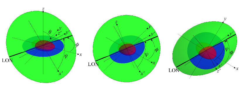
Figure 1: Schematic three-dimensional view of the ellipsoid geometry. The bulge ellipsoid, the disk plane, and the sky plane are shown in red, blue, and green, respectively. The reference systems of the ellipsoid and of the observer as well as the LON are plotted with thin solid lines, thin dashed lines, and a thick solid line, respectively. The bulge ellipsoid is shown as seen from an arbitrary viewing angle (left panel), along the LOS (central panel), and along the polar axis (i.e., the $z-$axis; right panel).

From the previous considerations (see Simonneau et al. 1998, for details) we have that the equations relating the length of the semi-axes of the projected ellipse with the length of the semi-axes of the intrinsic ellipsoid are given by

$$a^{2}b^{2} = A^{2}C^{2}\sin^{2}\theta\cos^{2}\phi+B^{2}C^{2}\sin^{2}\theta\sin^{2}\phi+A^{2}B^{2}\cos^{2}\theta,$$ (2)

$$a^{2}+b^{2} = A^{2}(\cos^{2}\phi+\cos^{2}\theta\sin^{2}\phi)+B^{2}(\sin^{2}\phi+\cos^{2}\theta\cos^{2}\phi)+C^{2}\sin^{2}\theta,$$ (3)

$$\tan 2\delta = \frac{(B^{2}-A^{2})\cos\theta\sin 2\phi}{A^{2}(\cos^{2}\theta\sin^{2}\phi-\cos^{2}\phi)+B^{2}(\cos^{2}\theta\cos^{2}\phi-\sin^{2}\phi)+C^{2}\sin^{2}\theta}.$$ (4)

If the ellipsoidal bulge is not circular in the equatorial plane ($A\neq B$) then it is possible to observe a twist ($\delta\neq 0$; see Eq. 4) between the axes of the projected ellipses of the bulge and disk.

2.2 Inverse problem: from ellipses to ellipsoids

We will focus now our attention on the inverse problem, i.e., the problem of deprojection. Following Simonneau et al. (1998), from Eqs. 2, 3, and 4, we are able to express the length of the bulge semi-axes ($A$, $B$, and $C$) as a function of the length of the semi-axes of the projected ellipse ($a$, $b$) and the twist angle ($\delta$).

For the sake of clarity, we rewrite here the corresponding equations but in a different way with respect to Paper I. First, we define

$$K^{2}=\frac{a^{2}+b^{2}}{2}\left[1+e\,\cos 2\delta\right],$$ (5)

where

$$e=\frac{a^{2}-b^{2}}{a^{2}+b^{2}}\qquad-1\leq e\leq 1,$$ (6)

is, in some sense, a measure of the ellipticity of the observed ellipse. Therefore, $K^{2}$ is a positive measurable quantity.

From Eqs. 2, 3, and 4 it results

$$K^{2}=\frac{A^{2}+B^{2}}{2}\left[1+E\,\cos 2\phi\right],$$ (7)

where

$$E=\frac{A^{2}-B^{2}}{A^{2}+B^{2}}\qquad-1\leq E\leq 1,$$ (8)

measures the intrinsic equatorial ellipticity of the bulge.

With this notation we can rewrite the equations for the semi-axes of the bulge in the form

$$A^{2} = K^{2}\left(1+\frac{e\,\sin 2\delta}{1+e\,\cos 2\delta}\frac{\tan\phi}{\cos\theta}\right),$$ (9)

$$B^{2} = K^{2}\left(1-\frac{e\,\sin 2\delta}{1+e\,\cos 2\delta}\frac{\cot{\phi}}{\cos\theta}\right),$$ (10)

$$C^{2} = K^{2}\left(1-\frac{2\,e\,\cos 2\delta}{\sin^{2}\theta\left(1+e\,\cos 2\delta\right)}+\frac{2\,e\,\cos\theta\,\sin 2\delta}{\sin^{2}\theta\left(1+e\,\cos 2\delta\right)}\cot^{2}{\phi}\right).$$ (11)

The values of $a,b,\delta,$ and $\theta$ can be directly obtained from observations. Unfortunately, the relation between the intrinsic and projected variables also depends on the spatial position of the bulge (i.e., on the $\phi$ angle), which is actually the unique unknown of our problem. Indeed, this will constitute the basis of our statistical analysis.

2.3 Characteristic angles

There are physical constraints which limit the possible values of $\phi$, such as the positive length of the three semi-axes of the ellipsoid (Simonneau et al. 1998). Therefore, we define some characteristic angles which constrain the range of $\phi$. Two different possibilities must be taken into account for any value of the observed variables $a$, $b$, $\delta$ and $\theta$.

The first case corresponds to $a>b$. It implies that $e>0$ from Eq. 6 and $A>B$ from Eqs. 9 and 10. For any value of $\phi$, $A^{2}>K^{2}$ and $K^{2}$ is always positive according to Eq. 7. On the other hand, $B^{2}$ and $C^{2}$ can be either positive or negative depending on the value of $\phi$ according to Eqs. 10 and 11, respectively. This limits the range of the values of $\phi$. $B^{2}$ is positive only for $\phi>\phi_{B}$. The angle $\phi_{B}$ is defined by $B^{2}=0$ in Eq. 10 as

$$\tan{\phi_{B}}=\frac{e\,\sin{2\delta}}{\cos{\theta}\,\left(1+e\,\cos{2\delta}\right)}.$$ (12)

Likewise, $C^{2}$ is positive only for values of $\phi<\phi_{C}$. The angle $\phi_{C}$ is defined by $C^{2}=0$ in Eq. 11 as

$$\tan{2\phi_{C}}=\frac{2\,e\,\sin{2\delta}\,\cos{\theta}}{e\,\cos{2\delta}\,\left(1+\cos^{2}{\theta}\right)-\sin^{2}{\theta}}.$$ (13)

Thus, if $a>b$ then the values of $\phi$ can only be in the range $\phi_{B}\leq\phi\leq\phi_{C}$.

The second case corresponds to $a<b$. It implies that $e<0$ (Eq. 6) and $A<B$ (Eqs. 9 and 10). For any value of $\phi$, $B^{2}>K^{2}$ and $K^{2}$ is always positive according to Eq. 7. But, $A^{2}$ and $C^{2}$ can be either positive or negative depending on the value of $\phi$ according to Eqs. 9 and 11, respectively. This limits the range of the values of $\phi$. $A^{2}$ is positive only for $\phi<\phi_{A}$. The angle $\phi_{A}$ is defined by $A^{2}=0$ in Eq. 9 as

$$\tan{\phi_{A}}=-\frac{\cos{\theta}\left(1+e\,\cos{2\delta}\right)}{e\,\sin{2\delta}}.$$ (14)

Likewise, $C^{2}$ is positive only for values of $\phi>\phi_{C}$. The angle $\phi_{C}$ is given in Eq. 13. Thus, if $a<b$, then the values $\phi$ can only be in the range $\phi_{C}\leq\phi\leq\phi_{A}$.

However, the problem is symmetric: the second case, when the first semi-axis of the observed ellipse (which is measured clockwise from the LON) corresponds to the minor axis (i.e., $a<b$), is the mirror situation of the first case, when the first measured semi-axis of the observed ellipse corresponds to the major axis (i.e., $a>b$). In the second case, if we assume the angle $\pi/2-\delta$ to define the position of the major semi-axis $a$ of the observed ellipse with respect to the LON in the sky plane, and $\pi/2-\phi$ to define the position of the major semi-axis $A$ of the equatorial ellipse of the bulge with respect to the LON in the bulge equatorial plane, then we can always consider $a>b$ and $A>B$. Therefore, $e\geq 0$ and $E\geq 0$ always. This means that we have the same mathematical description in both cases: the possible values of $\phi$ are $\phi_{B}\leq\phi\leq\phi_{C}$ with $\phi_{B}$ and $\phi_{C}$ defined by Eqs. 12 and 13, respectively. Furthermore, we can rewrite Eqs. 9, 10, and 11

$$A^{2} = K^{2}\left[1+\tan{\phi_{B}}\,\tan{\phi}\right],$$ (15)

$$B^{2} = K^{2}\left[1-\frac{\tan{\phi_{B}}}{\tan{\phi}}\right],$$ (16)

$$C^{2} = K^{2}\,2\,\tan{\phi_{B}}\frac{\cos^{2}\theta}{\sin^{2}\theta}\left[\cot{2\,\phi}-\cot{2\,\phi_{C}}\right].$$ (17)

where $\phi_{B}$ and $\phi_{C}$ are given as a function of the observed variables $a$, $b$, $\delta$, and $\theta$, i.e., they are known functions for each observed bulge.

We can always consider $A>B$ as explained before. But, we are not imposing any constraint on the length $C$ of the polar semi-axis. According to this definition oblate and prolate triaxial ellipsoids do not necessarily have an axisymmetric shape. We will define a triaxial ellipsoid as completely oblate if $C$ is smaller than both $A$ and $B$ (i.e., the polar axis is the shortest axis of the ellipsoid). We define a triaxial ellipsoid as completely prolate if $C$ is greater than both $A$ and $B$ (i.e., the polar axis is the longest axis of the ellipsoid). If the polar axis is the intermediate axis we have either a partially oblate or a partially prolate triaxial ellipsoid. A further detailed description of all these cases will be given at the end of this section.

From Eq. 16 we obtain that the semi-axis length $B$ is zero for $\phi=\phi_{B}$ and it increases when $\phi$ goes from $\phi_{B}$ to $\phi_{C}$. The semi-axis length $C$ is zero for $\phi=\phi_{C}$ and decreases when $\phi$ goes from $\phi_{B}$ to $\phi_{C}$. There is an intermediate value $\phi_{BC}$ for which $B^{2}=C^{2}$. This angle is given by

$$\tan{\phi_{BC}}=\frac{\tan{\delta}}{\cos{\theta}}.$$ (18)

For $\phi_{BC}<\phi<\phi_{C}$, $C^{2}<B^{2}$ and both of them are smaller than $A^{2}$. This implies that in this range of $\phi$ the corresponding triaxial ellipsoid is completely oblate.

On the other hand, $B^{2}<A^{2}$ for all possible values of $\phi$. This is not the case for $C^{2}$, because it increases when $\phi$ decreases. Thus, we can define a new angle $\phi_{AC}$ for which $C^{2}=A^{2}$. This angle is given by

$$\tan{\phi_{AC}}=\cos{\theta}\tan{\delta}.$$ (19)

For $\phi<\phi_{AC}$, $C^{2}>A^{2}>B^{2}$. Therefore, the corresponding triaxial ellipsoid is completely prolate. It is important to notice here that this case is physically possible only when $\phi_{AC}>\phi_{B}$, and the values of $\phi$ are within the range of possible values $\phi_{B}\leq\phi\leq\phi_{C}$. Therefore, we conclude that for any observed bulge (i.e., for any set of measured values of $a$, $b$, $\delta$, and $\theta$) the corresponding triaxial ellipsoid could be always completely oblate, while we are not sure that it could be prolate.

We define the quadratic mean radius of the equatorial ellipse of the bulge in order to extensively discuss all the different possibilities.

$$R^{2}=\frac{A^{2}+B^{2}}{2}=K^{2}\tan{\phi_{B}}\left[\cot{\phi_{B}}-\cot{2\,\phi}\right],$$ (20)

which depends only on the unknown position $\phi$.

Since $A^{2}>B^{2}$, $A^{2}\geq R^{2}\geq B^{2}$ but there is always a value $\phi_{\rm RC}$ corresponding to the case $C^{2}=R^{2}$

$$\tan{2\phi_{RC}}=\tan{2\delta}\,\frac{1+\cos^{2}{\theta}}{2\,\cos{\theta}}.$$ (21)

The mean equatorial radius allows us to distinguish oblate ($C^{2}<R^{2}$) and prolate ($C^{2}>R^{2}$) triaxial ellipsoids. Unfortunately, the situation is more complicated and there are four different possibilities for the intrinsic shape of the bulge ellipsoid. They are sketched in Fig. 2 and can be described as follows

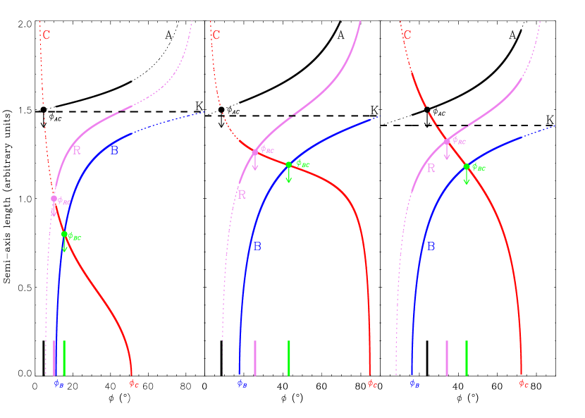
Figure 2: The lengths $A$, $B$, and $C$ of the semi-axes of the bulge ellipsoid and its mean equatorial radius $R$ as a function of the angle $\phi$. The solid lines correspond to the ranges of physically possible values of $A$, $B$, $C$, and $R$, while the dotted lines show their overall trends within $0\leq\phi\leq\pi/2$. A triaxial bulge with $\phi_{AC}<\phi_{RC}<\phi_{B}$, $\phi_{AC}<\phi_{B}<\phi_{RC}$, and $\phi_{B}<\phi_{AC}<\phi_{RC}$ is shown in the left, central, and right panel, respectively.

• If $\phi_{AC}<\phi_{RC}<\phi_{B}$ the triaxial ellipsoid is always oblate (Fig. 2, left panel). It is either completely oblate (i.e., $A>B>C$) if $R>B>C$ ($\phi_{BC}<\phi<\phi_{C}$) or partially oblate if $R>C>B$ ($\phi_{B}<\phi<\phi_{BC}$).

• If $\phi_{AC}<\phi_{B}<\phi_{RC}$ the triaxial ellipsoid can be either oblate or prolate (Fig. 2, central panel). It is either completely oblate if $R>B>C$ ($\phi_{BC}<\phi<\phi_{C}$), or partially oblate if $R>C>B$ ($\phi_{RC}<\phi<\phi_{BC}$), or partially prolate if $C>R>B$ ($\phi_{B}<\phi<\phi_{RC}$).

• If $\phi_{B}<\phi_{AC}<\phi_{RC}$ four different possibilities are allowed for the triaxial shape of the bulge ellipsoid (Fig. 2, right panel). It is either completely oblate if $R>B>C$ ($\phi_{BC}<\phi<\phi_{C}$), or partially oblate if $R>C>B$ ($\phi_{RC}<\phi<\phi_{BC}$), or partially prolate if $A>C>R$ ($\phi_{AC}<\phi<\phi_{BC}$), or completely prolate (i.e., $C>A>B$) if $C>A>R$ ($\phi_{B}<\phi<\phi_{AC}$).

3 Equatorial ellipticity of bulges

In Paper I we focused on the equatorial ellipticity defined in Eq. 8. This is a straightforward definition resulting from the equations involved in projecting and deprojecting triaxial ellipsoids. It allows us to solve the problem of inverting an integral equation in order to derive the PDF of the equatorial ellipticity of bulges. However, the usual axial ratio $B/A$ is a more intuitive choice to describe the equatorial ellipticity of the bulge when only one galaxy is considered. Therefore, we redefine the equatorial ellipticity as $Z=B^{2}/A^{2}$. Adopting a squared quantity gives us the chance of successfully performing an analytic study of the problem. By taking into account Eqs. 15 and 16, we obtain

$$Z=\frac{B^{2}}{A^{2}}=\frac{\tan{\left(\phi-\phi_{B}\right)}}{\tan{\phi}}=1-\frac{2\,\sin{\phi_{B}}}{\sin{\phi_{B}}+\sin{\left(2\phi-\phi_{B}\right)}}.$$ (22)

$Z=0$ for $\phi=\phi_{B}$, while the limiting value of $Z$ for $\phi=\phi_{C}$ is

$$Z_{C}=\frac{\tan{\left(\phi_{C}-\phi_{B}\right)}}{\tan{\phi_{C}}}=1-\frac{2\,\sin{\phi_{B}}}{\sin{\phi_{B}}+\sin{\left(2\,\phi_{C}-\phi_{B}\right)}}.$$ (23)

When $\phi$ is between $\phi_{B}$ and $\phi_{C}$, the value of $Z$ reaches a maximum given by

$$Z_{\rm M}=\frac{1-\sin{\phi_{B}}}{1+\sin{\phi_{B}}},$$ (24)

which is observed when $\phi$ corresponds to

$$\phi_{\rm M}=\frac{\pi}{4}+\frac{\phi_{B}}{2},$$ (25)

where $\phi_{\rm M}$ is always larger than $\phi_{B}$. The value $Z$ decreases for $\phi>\phi_{\rm M}$, after reaching its maximum $Z_{\rm M}$ at $\phi=\phi_{\rm M}$. $Z=0$ for $\phi=\pi/2$. But, it is not necessary to study the behaviour of $Z$ for $\phi_{C}<\phi\leq\pi/2$ since this range of $\phi$ is not physically possible.

Therefore, as soon as $\phi$ increases from $\phi_{B}$ to $\phi_{C}$ there are two possible cases for $\phi_{\rm M}$ and the corresponding trend of $Z$. If $\phi_{C}>\phi_{\rm M}$, the value of $Z$ reaches the maximum $Z_{\rm M}$ for $\phi=\phi_{\rm M}$. For larger values of $\phi$ it decreases, reaching the limit value $Z_{C}$ for $\phi=\phi_{C}$. If $\phi_{C}<\phi_{\rm M}$, $Z$ does not reach the maximum value given by Eq. 24. In this case, the maximum value of $Z$ corresponds to $Z_{C}$.

We also derive for each observed bulge the mean value $\langle Z\rangle$ of its equatorial ellipticity. From Eq. 22

$$\langle Z\rangle = \frac{1}{\phi_{C}-\phi_{B}}\int_{\phi_{B}}^{\phi_{C}}Z(\phi)\,d\phi=$$ (26)

$$= 1\,-\frac{\tan{\phi_{B}}}{\phi_{C}-\phi_{B}}\ln{\frac{\sin{\phi_{C}}}{\cos{\left(\phi_{C}-\phi_{B}\right)\,\sin{\phi_{B}}}}}.$$

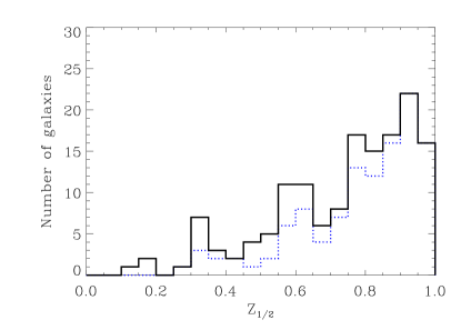
Figure 3: The distribution of the 148 sample bulges as a function of their maximum (top panel), mean (middle panel), and median (bottom panel) equatorial ellipticities plotted with a solid line. In each panel, the dotted line refers to the distribution of the 115 sample bulges with $\phi_{C}>\phi_{\rm M}$.

To perform a more exhaustive statistical analysis, we compute for each observed bulge the probability $P(Z)$ corresponding to $0<Z<Z_{C}$ by taking into account that $\phi$ can take any value in the range $\phi_{B}\leq\phi\leq\phi_{C}$ with the same probability given by

$$P(\phi)=\frac{1}{\phi_{C}-\phi_{B}}.$$ (27)

$P(Z)=\sum P(\phi)\left|d\phi/dZ\right|$, where the sum is defined over all the $\phi$ values which solve Eq. 22. The probability $P(Z)$ allows us to compute some characteristic values of $Z$, such as the median value $Z_{1/2}$. It is defined in such a way that the integrated probability between $Z=0$ and $Z_{1/2}$ is equal to the integrated probability between $Z_{1/2}$ and $Z_{C}$.

The distribution of the sample bulges as a function of their maximum, mean, and median equatorial ellipticity is plotted in Fig. 3.

Moreover, we define the confidence interval ($Z_{1/6},Z_{5/6}$) where the integrated probability is 67%. The integrated probabilities between $Z=0$ and $Z_{1/6}$ and between $Z=0$ and $Z_{5/6}$ are 1/6 and 5/6, respectively. To this aim, we introduce three characteristic values of $\phi$ in the range between $\phi_{B}$ and $\phi_{C}$. According to the probability $P(\phi)$ given in Eq. 27, they are

$$\phi^{0}_{1/2}=\frac{1}{2}\phi_{C}+\frac{1}{2}\phi_{B},$$ (28)

$$\phi^{0}_{1/6}=\frac{1}{6}\phi_{C}+\frac{5}{6}\phi_{B},$$ (29)

$$\phi^{0}_{5/6}=\frac{5}{6}\phi_{C}+\frac{1}{6}\phi_{B}.$$ (30)

We have seen that $Z$ has a different behaviour for $\phi_{C}<\phi_{\rm M}$ and for $\phi_{C}>\phi_{\rm M}$. Therefore, we will separately study these two cases in order to derive $P(Z)$ and the corresponding distribution of equatorial ellipticities.

3.1 Bulges with $\phi_{C}<\phi_{\rm M}$

If $\phi_{C}<\phi_{\rm M}$, the value of $Z$ monotonically increases from $Z(\phi_{\rm B})=0$ to $Z_{C}=Z(\phi_{C})$. There is only one value of $\phi$ corresponding to any given value of $Z$. Thus the integrated probability $P(Z)$ from $Z=0$ to $Z=Z_{1/6}$, $Z_{1/2}$, and $Z_{5/6}$ is equal to the integration of $P(\phi)$ from $\phi=\phi_{B}$ to $\phi=\phi^{0}_{1/6}$, $\phi^{0}_{1/2}$, and $\phi^{0}_{5/6}$, respectively. Consequently, the median value is

$$Z_{1/2}=Z(\phi^{0}_{1/2})=1-\frac{2\,\sin{\phi_{B}}}{\sin{\phi_{B}}+\sin{\phi_{C}}},$$ (31)

and the limits of the confidence interval are

$$Z_{1/6}=Z(\phi^{0}_{1/6})=1-\frac{2\,\sin{\phi_{B}}}{\sin{\phi_{B}}+\sin{\left(\frac{1}{3}\phi_{C}+\frac{2}{3}\phi_{B}\right)}},$$ (32)

and

$$Z_{5/6}=Z(\phi^{0}_{5/6})=1-\frac{2\,\sin{\phi_{B}}}{\sin{\phi_{B}}+\sin{\left(\frac{5}{3}\phi_{C}-\frac{2}{3}\phi_{B}\right)}}.$$ (33)

In this case, the probability $P(Z)$ is

$$P(Z)=\frac{1}{\phi_{C}-\phi_{B}}\,\frac{\sin{\phi_{B}}}{(1-Z)\,\sqrt{(1-Z)^{2}-\sin^{2}{\phi_{B}}\,(1+Z)^{2}}},$$ (34)

which increases monotonically between

$$P(0)=\frac{1}{\phi_{C}-\phi_{B}}\,\tan{\phi_{B}},$$ (35)

and

$$P(Z_{C})=\frac{1}{\phi_{C}-\phi_{B}}\,\frac{1}{4}\,\frac{\left[\sin{\phi_{B}}+\sin{\left(2\,\phi_{C}-\phi_{B}\right)}\right]^{2}}{\sin{\phi_{B}\,\cos{\left(2\,\phi_{C}-\phi_{B}\right)}}}.$$ (36)

The probability $P(Z)$ given in Eq. 34 strongly peaks at $Z=Z_{C}$ in such a way that $Z_{1/2}$ is close to $Z_{C}$. For this reason, although the right portion ($Z_{1/2},Z_{5/6}$) of the confidence interval ($Z_{1/6},Z_{5/6}$) is not large, the confidence interval spans a large fraction of the total range between 0 and $Z_{C}$. This is the case for the bulge of MCG -02-33-017 (Fig. 4, top panel). Using the mean $\langle Z\rangle$ and median $Z_{1/2}$ values to describe the equatorial ellipticity of these kinds of bulges is a poor approximation.

Figure 4: PDF of the equatorial ellipticity for three sample bulges. MCG -02-33-017 (top panel) hosts a bulge with $\phi_{C}<\phi_{\rm M}$. NGC 1107 (middle panel) hosts a bulge with $\phi_{C}>\phi_{\rm M}$ and $\phi^{0}_{1/2}<\phi^{\prime}_{C}$. NGC 4789 (bottom panel) hosts a bulge with $\phi_{C}>\phi_{\rm M}$ and $\phi^{0}_{1/2}>\phi^{\prime}_{C}$. In each panel, the vertical line shows the median $Z_{1/2}$ value, the arrow corresponds to the maximum value of $Z$, and the hatched area marks the confidence interval ($Z_{1/6},Z_{5/6}$) corresponding to $67\%$ probability.

3.2 Bulges with $\phi_{C}>\phi_{\rm M}$

For $\phi_{C}>\phi_{\rm M}$, $Z$ monotonically increases from $Z(\phi_{B})=0$ to $Z_{\rm M}=Z(\phi_{\rm M})$ and then it monotonically decreases from $Z_{\rm M}$ to $Z_{C}=Z(\phi_{C})$. For $0<Z<Z_{C}$ there is only one value of $\phi$ for each value of $Z$, while for $Z_{C}<Z<Z_{\rm M}$ there are two values of $\phi$ which correspond to each value of $Z$. There is a discontinuity in $P(Z)$ for $Z=Z_{C}$, which corresponds to the value $\phi^{\prime}_{C}=\frac{\pi}{2}-(\phi_{C}-\phi_{B})$. $dZ/d\phi=0$ for $\phi=\phi_{\rm M}$ and the probability $P(Z)$ becomes infinity at $Z=Z_{\rm M}$. It is not possible to compute directly the median value $Z_{1/2}$ and confidence interval ($Z_{1/6},Z_{5/6}$) from $P(\phi)$ in Eq. 27. Therefore, we need to rewrite $P(Z)$ as

$$P(Z)=\left\{\begin{array}[]{l}\frac{1}{\phi_{C}-\phi_{B}}\,\frac{\sin{\phi_{B}}}{(1-z)\,\sqrt{(1-z)^{2}-\sin^{2}{\phi_{B}}\,(1+z)^{2}}}\qquad 0\leq Z<Z_{C},\\ \frac{2}{\phi_{C}-\phi_{B}}\,\frac{\sin{\phi_{B}}}{(1-z)\,\sqrt{(1-z)^{2}-\sin^{2}{\phi_{B}}\,(1+z)^{2}}}\qquad Z_{C}\leq Z\leq Z_{\rm M}.\\ \end{array}\right.$$ (39)

There are different values for $Z_{1/6}$, $Z_{1/2}$, and $Z_{5/6}$ depending on whether $\phi^{0}_{1/2}$ is smaller or greater than $\phi^{\prime}_{C}$ which corresponds to the discontinuity in $P(Z)$.

For $\phi^{0}_{1/2}<\phi^{\prime}_{C}$ the values of $Z_{1/2}$ and $Z_{1/6}$ are given by Eqs. 31 and 32, respectively. But, there are two possible values for $Z_{5/6}$ depending on the value of $\phi^{0}_{5/6}$. If $\phi^{0}_{5/6}<\phi^{\prime}_{C}$ then $Z_{5/6}$ is given by the Eq. 33. If $\phi^{0}_{5/6}>\phi^{\prime}_{C}$ the corresponding values of $Z$ are on the right side of the discontinuity (i.e., two values of $Z$ correspond to a given value of $\phi>\phi^{\prime}_{C}$). In this case

$$Z_{5/6}=1-\frac{2\,\sin{\phi_{B}}}{\sin{\phi_{B}}+\cos{\frac{\phi_{C}-\phi_{B}}{6}}},$$ (40)

which corresponds to $Z(\phi_{5/6})$ with $\phi_{5/6}=\pi/4-\phi_{C}/12+7\,\phi_{B}/12$.

For $\phi^{0}_{1/2}>\phi^{\prime}_{C}$ the value of $Z_{1/2}$ is given by

$$Z_{1/2}=1-\frac{2\,\sin{\phi_{B}}}{\sin{\phi_{B}}+\cos{\frac{\phi_{C}-\phi_{B}}{2}}},$$ (41)

and it corresponds to $Z(\phi_{1/2})$ with $\phi_{1/2}=\pi/2-\phi_{C}/2+3\,\phi_{B}/2$. Likewise, $Z_{5/6}$ is given by Eq. 40. But, for $Z_{1/6}$ we have two possibilities according to the value of $\phi^{0}_{1/6}$. If $\phi^{0}_{1/6}<\phi^{\prime}_{C}$ then $Z_{1/6}$ is given by Eq. 32. If $\phi^{0}_{1/6}>\phi^{\prime}_{C}$ the corresponding values of $Z$ are on the right side of the discontinuity, and it is

$$Z_{1/6}=1-\frac{2\,\sin{\phi_{B}}}{\sin{\phi_{B}}+\cos{\frac{5\,\left(\phi_{C}-\phi_{B}\right)}{6}}}$$ (42)

which corresponds to $Z(\phi_{1/6})$ with $\phi_{1/6}=\pi/4-5\,\phi_{C}/12+11\,\phi_{B}/12$.

For $\phi_{C}>\phi_{\rm M}$ the probability $P(Z)$ in Eq. 39 peaks strongly at $Z_{\rm M}$ and therefore the median $Z_{1/2}$ and maximum $Z_{\rm M}$ values of the equatorial ellipticity are very close and the confidence interval ($Z_{1/6},Z_{5/6}$) is narrow. This is the case for the bulges of NGC 1107 (Fig. 4, middle panel) and NGC 4789 (Fig. 4, bottom panel). We conclude that for these types of bulges the statistics we have presented here are representative of their intrinsic equatorial ellipticity.

3.3 Statistics of the equatorial ellipticity of bulges

The distribution of the maximum equatorial ellipticity (corresponding to either $Z_{C}$ for bulges with $\phi_{C}<\phi_{\rm M}$ or $Z_{\rm M}$ for bulges with $\phi_{C}>\phi_{\rm M}$) peaks at $Z_{\rm M}>0.9$ (Fig. 3, top panel). These are nearly circular bulges ($B/A=0.95$). But, we conclude that a large fraction of the sample bulges are strong candidates to be triaxial because $41\%$ of them have $Z_{\rm M}<0.80$ ($B/A<0.89$). This result is in agreement with our previous finding in Paper I and with the analysis of the distribution of mean (Fig. 3, middle panel) and median (Fig. 3, bottom panel) ellipticities. In fact, we find that $64\%$ and $53\%$ of our bulges have $\langle Z\rangle<0.8$ and $Z_{1/2}<0.8$, respectively. The mean values of $\langle Z\rangle$ and $Z_{1/2}$ are 0.68 and 0.73, respectively.

The width of the confidence interval ($Z_{1/6},Z_{5/6}$) corresponding to a $67\%$ probability is related to the accuracy of the $Z$ measurement. The narrowest confidence intervals are found for bulges with $\phi_{C}\rightarrow\pi/2$ and $\phi_{B}\rightarrow 0$. This implies that $\phi^{\prime}_{C}\rightarrow\phi_{B}$ and $Z_{C}>Z_{\rm M}$. For these bulges the discontinuity in $P(Z)$ is almost negligible. The case with $\phi_{C}=\pi/2$ and $\phi_{B}=0$ corresponds either to spherical bulges (i.e., $e=0$) or to bulges with a circular equatorial section (i.e., $\tan{2\delta}=0$). Consequently, the bulges with $B\approx A$ are among those characterized by the narrower confidence interval and better determination of $Z$. We can select all sample objects for which the $Z$ measurement is only slightly uncertain. They are the 115 galaxies with $\phi_{C}>\phi_{\rm M}$. The distribution of these selected bulges as a function of their $Z_{\rm M}$, $\langle Z\rangle$, and $Z_{1/2}$ is plotted in Fig. 3 too. The fraction of bulges with $Z_{\rm M}<0.8$ is $33\%$. It is significantly smaller than the $41\%$ found for the complete sample, because the selected sample is biased toward bulges with $B\approx A$ including all the bulges with a circular (or nearly circular) equatorial section. The fraction of selected bulges with $\langle Z\rangle<0.8$ and $Z_{1/2}<0.8$ is $55\%$ and $43\%$, respectively.

4 Intrinsic flattening of bulges

The axial ratio $C/A$ usually describes the intrinsic flattening $F$ of a triaxial ellipsoid if $A\geq B\geq C$. Since we have no constraints on the lengths $A$, $B$, and $C$, we redefine the flattening as

$$F(\phi)=\frac{C^{2}}{R^{2}}=\frac{2C^{2}}{A^{2}+B^{2}},$$ (43)

by using the lengths $C$ and $R$ of the polar semi-axis and the mean equatorial radius given by Eqs. 11 and 20, respectively.

$$F(\phi)=F_{\theta}\,\frac{\cot{2\phi}-\cot{2\phi_{C}}}{\cot{\phi_{B}}-\cot{2\phi}}=F_{\theta}\,\frac{\sin{\phi_{B}}}{\sin{2\phi_{C}}}\frac{\sin{\left(2\phi_{C}-2\phi\right)}}{\sin{\left(2\phi-\phi_{B}\right)}},$$ (44)

where

$$F_{\theta}=\frac{2\,\cos^{2}{\theta}}{\sin^{2}{\theta}},$$ (45)

accounts for the effect of inclination. The angle $\theta$ also enters in the definition of the two angles $\phi_{B}$ and $\phi_{C}$ in Eqs. 12 and 13, respectively. Adopting a squared quantity for $F$ gives us the chance of successfully performing an analytic study of the problem as was done for the equatorial ellipticity $Z$ in Eq. 22.

Since $dF(\phi)/d\phi<0$, the function $F(\phi)$ is monotonically decreasing with a maximum $F_{\rm M}$ at $\phi=\phi_{B}$ given by

$$F_{\rm M}=F_{\theta}\frac{\sin{\left(2\,\phi_{C}-2\,\phi_{B}\right)}}{\sin{2\,\phi_{C}}}.$$ (46)

If $\phi$ increases from $\phi_{B}$ to $\phi_{C}$, the value of $F(\phi)$ decreases to zero at $\phi=\phi_{C}$. According to Eq. 46, for $F_{\rm M}<1$ the triaxial ellipsoids are oblate, with some of them being partially oblate and others completely oblate. For $F_{\rm M}>1$ the triaxial ellipsoids can also be partially prolate and in some extreme cases completely prolate.

From Eq. 44, we compute the mean value $\langle F\rangle$ of the intrinsic flattening as

$$\langle F\rangle = \frac{1}{\phi_{C}-\phi_{B}}\int_{\phi_{B}}^{\phi_{C}}F(\phi)\,d\phi=$$ (47)

$$= F_{\theta}\frac{\sin{\phi_{B}}}{\sin{2\,\phi_{C}}}\left[\frac{\sin{\left(2\,\phi_{C}-\phi_{B}\right)}}{2\,\left(\phi_{C}-\phi_{B}\right)}\ln{\left(\frac{\sin{\left(2\,\phi_{C}-\phi_{B}\right)}}{\sin{\phi_{B}}}\right)}-\right.$$

$$\left.-\cos{\left(2\,\phi_{C}-\phi_{B}\right)}\right].$$

Since $F(\phi)$ is a monotonic function (i.e., each value of $F$ corresponds to only one value of $\phi$), the integrated probability $P(F)$ between $F(\phi_{C})=0$ and some characteristic value $F_{*}=F(\phi_{*})$ is equal to the integral of $P(\phi)$ between $\phi_{*}$ and $\phi_{C}$. Then, it is straightforward to compute the median value $F_{1/2}$ of the intrinsic flattening which corresponds to the median value $\phi^{0}_{1/2}=(\phi_{C}+\phi_{B})/2$

$$F_{1/2}=F_{\theta}\,\frac{\sin{\phi_{B}}}{\sin{\left(2\,\phi_{C}\right)}}\frac{\sin{\left(\phi_{C}-\phi_{B}\right)}}{\sin{\phi_{C}}}.$$ (48)

As was done for the equatorial ellipticity, we can define also for the flattening a confidence interval ($F_{1/6}$, $F_{5/6}$) where the integrated probability is $67\%$. In fact, the integrated probabilities between $F=0$ and $F_{1/6}$ and between $F=0$ and $F_{5/6}$ are 1/6 and 5/6, respectively. We have

$$F_{1/6}=F_{\theta}\,\frac{\sin{\phi_{B}}}{\sin{\left(2\,\phi_{C}\right)}}\frac{\sin{\left(\frac{1}{3}\phi_{C}-\frac{1}{3}\phi_{B}\right)}}{\sin{\left(\frac{5}{3}\phi_{C}-\frac{2}{3}\phi_{B}\right)}},$$ (49)

which corresponds to $\phi^{0}_{1/6}$ given in Eq. 29, and

$$F_{5/6}=F_{\theta}\,\frac{\sin{\phi_{B}}}{\sin{\left(2\,\phi_{C}\right)}}\frac{\sin{\left(\frac{5}{3}\phi_{C}-\frac{5}{3}\phi_{B}\right)}}{\sin{\left(\frac{1}{3}\phi_{C}+\frac{2}{3}\phi_{B}\right)}},$$ (50)

which corresponds to $\phi^{0}_{5/6}$ given in Eq. 30. The distribution of the sample bulges as a function of their maximum, mean, and median intrinsic flattening is plotted in Fig. 5.

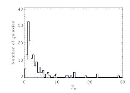
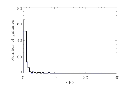
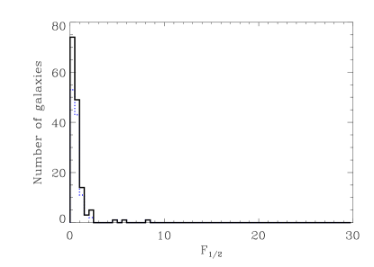
Figure 5: The distribution of the 148 sample bulges as a function of their maximum (top panel), mean (middle panel), and median (bottom panel) intrinsic flattening, plotted with a solid line. In each panel, the dotted line refers to the distribution of the 115 sample bulges with $\phi_{C}>\phi_{\rm M}$.

It is possible to perform a more exhaustive statistical analysis by defining the probability $P(F)$ of having a flattening $F$ as

$$P(F)=k_{0}\,\frac{1}{A_{0}F^{2}+B_{0}F+C_{0}},$$ (51)

where

$$k_{0} = \frac{\cos^{2}{\theta}\,\sin{\left(2\phi_{C}-\phi_{B}\right)}}{\sin^{2}{\theta}\,(\phi_{C}-\phi_{B})\,\sin{2\phi_{C}}\,\sin{\phi_{B}}},$$ (52)

$$A_{0} = \frac{1}{\sin^{2}{\phi_{B}}},$$ (53)

$$B_{0} = \frac{4\,\cos^{2}{\theta}\,\cos{\left(2\phi_{C}-\phi_{B}\right)}}{\sin^{2}{\theta}\,\sin{2\phi_{C}}\,\sin{\phi_{B}}},$$ (54)

$$C_{0} = \frac{4\,cos^{4}{\theta}}{\sin^{4}{\theta}\,\sin^{2}{2\phi_{C}}},$$ (55)

where $k_{0}$, $A_{0}$, and $C_{0}$ are always positive, while $B_{0}>0$ for $2\phi_{C}-\phi_{B}<\pi/2$ ($\phi_{C}<\phi_{\rm M}$) and $B_{0}<0$ for $2\phi_{C}-\phi_{B}>\pi/2$ ($\phi_{C}>\phi_{\rm M}$). All these quantities can be computed directly for each observed bulge, indeed they depend only on the measured values of $a$, $b$, $\delta$, and $\theta$ through the angles $\phi_{B}$ and $\phi_{C}$.

In Sect. 3.1 we found that the confidence interval ($Z_{1/6}$, $Z_{5/6}$) of equatorial ellipticity for a bulge with $\phi_{C}<\phi_{\rm M}$ is wide. For this reason, the median $Z_{1/2}$ and mean $\langle Z\rangle$ values are not representative of the equatorial ellipticity of the bulge. The same is true for ($F_{1/6}$, $F_{5/6}$) because the probability function $P(F)$ peaks at $F=0$ and slowly decreases as soon as $F$ increases. As a consequence, the median $F_{1/2}$ and mean $\langle F\rangle$ values are not representative of the intrinsic flattening of the bulge. This is the case for the bulge of MCG -02-33-017 (Fig. 6, left panels)

Figure 6: The intrinsic flattening as a function of the angle $\phi$ (top panels) and its PDF (bottom panels) for two sample bulges. MCG -02-33-017 (left panels) and NGC 4789 (right panels) host a bulge with $B_{0}>0$ and $B_{0}<0$, respectively. In the bottom panels, the vertical line shows the median $F_{1/2}$ value and the hatched area marks the confidence interval ($F_{1/6},F_{5/6}$) corresponding to $67\%$ of probability.

On the contrary, if $\phi_{C}>\phi_{\rm M}$ then $B_{0}<0$, and the probability function $P(F)$ peaks at the most probable value

$$F_{\rm MP}=-\frac{1}{2}\frac{B_{0}}{A_{0}},$$ (57)

and it quickly decreases to

$$P(0)=\frac{k_{0}}{C_{0}},$$ (58)

and to zero for $F<F_{\rm MP}$ and $F>F_{\rm MP}$, respectively. The confidence interval ($F_{1/6}$, $F_{5/6}$) is narrow. The median $F_{1/2}$, mean $\langle F\rangle$, and the most probable value $F_{\rm MP}$ are close to each other and all of them are representative of the intrinsic flattening. This is the case for the bulge of NGC 4789 (Fig. 6, right panels).

4.1 Statistics of the intrinsic flattening of bulges

The distribution of the maximum intrinsic flattening (Fig. 5, top panel) shows that $12\%$ of the sample bulges have $F_{\rm M}<1$ (i.e., they are either completely or partially oblate triaxial ellipsoids). Judging by $F_{\rm M}$, the majority of sample bulges could be highly elongated along the polar axis. However, these highly elongated bulges are not common. Indeed, after excluding from the complete sample the bulges with $F_{\rm M}<1$, only $19\%$ ($18\%$ if we consider only the selected sample of 115 bulges) of the remaining bulges have a probability greater than $50\%$ to have an intrinsic flattening $F>1$ and there are no bulges with more than a $90\%$ probability of having $F>1$ (Fig. 7). This is in agreement with the results based on the analysis of the distribution of the mean (Fig. 5, middle panel) and median (Fig. 5, bottom panel) intrinsic flattening. We find that $78\%$ of the sample bulges have $\langle F\rangle<1$, and $83\%$ have $F_{1/2}<1$. They are oblate triaxial ellipsoids.

The large number of sample bulges with $F_{\rm M}>1$ with respect to those which are actually elongated along the polar axis is due to a projection effect of the triaxial ellipsoids. For any $\phi$ the contribution of inclination $\theta$ to the value of $F$ is given by $F_{\theta}$ as defined in Eq. 45. However, the intrinsic flattening scales with $F_{\theta}$, whereas the probability $P(F)$ scales with $1/F_{\theta}$. Thus, the probability to have large $F_{\theta}$ values (and large $F_{\rm M}$ values) is very small. For instance, the probability to have the maximum $F_{\rm M}$ value given by Eq. 46 is

$$P(F_{\rm M})=\frac{1}{2\,\left(\phi_{C}-\phi_{B}\right)}\frac{1}{F_{\theta}}\frac{\sin{\phi_{B}}\,\sin{2\,\phi_{C}}}{\sin{\left(2\,\phi_{C}-\phi_{B}\right)}}.$$ (59)

We conclude that $F_{\rm M}$ is not a good proxy for the intrinsic flattening of a bulge, although $Z_{\rm M}$ is a good proxy for equatorial ellipticity.

Figure 7: Number of sample bulges which could have an intrinsic flattening $F>1$ as a function of the probability that this happens. Bulges with $F<1$ (i.e., oblate triaxial ellipsoids) have been not taken into account.

The distribution of the selected bulges with $\phi_{C}>\phi_{\rm M}$ as a function of their $F_{\rm M}$, $\langle F\rangle$, and $F_{1/2}$ is also plotted in Fig. 5. The fraction of oblate triaxial ellipsoids is rather similar to that of the complete sample, being $10\%$, $78\%$, and $83\%$ if we consider bulges with $F_{\rm M}<1$, $\langle F\rangle<1$, and $F_{1/2}<1$, respectively. The mean values of $\langle F\rangle$ and $F_{1/2}$ are 0.88 and 0.71, respectively, for the complete sample, and 0.86 and 0.75, respectively, for the selected sample.

5 Intrinsic shape of bulges

The distributions of the equatorial ellipticity and intrinsic flattening of bulges have been studied in Sects. 3 and 4 as two independent and not correlated statistics. It is possible to find the relation between them from Eqs. 8 and 43

$$\sqrt{E^{2}-\sin^{2}{\phi_{B}}}=\frac{\frac{F}{F_{\rm\theta}}\sin{2\phi_{C}}+\sin{\phi_{B}}\cos{\left(2\phi_{C}-\phi_{B}\right)}}{\sin{\left(2\,\phi_{C}-\phi_{B}\right)}},$$ (60)

to constrain the intrinsic shape of an observed bulge with the help of the known characteristic angles $\phi_{B}$ and $\phi_{C}$, which depend only on the measured values of $a$, $b$, $\delta$, and $\theta$. Eq. 60 can be rewritten as a function of the axial ratios $B/A$ and $C/A$ as

$$\frac{2\,\sin{\left(2\phi_{C}\right)}}{F_{\rm\theta}}\frac{C^{2}}{A^{2}}=$$

$$\sin{\left(2\phi_{C}-\phi_{B}\right)}\sqrt{\left(1-\frac{B^{2}}{A^{2}}\right)^{2}-\sin^{2}{\phi_{B}}\left(1+\frac{B^{2}}{A^{2}}\right)^{2}}-$$

$$\sin{\phi_{B}}\cos{\left(2\phi_{C}-\phi_{B}\right)}\left(1+\frac{B^{2}}{A^{2}}\right)^{2}.$$ (61)

Since $B/A$ and $C/A$ are both functions of the same variable $\phi$, their probabilities are equivalent (i.e., for a given value of $B/A$ with probability $P(B/A)$, the corresponding value of $C/A$ obtained by Eq. 61 has a probability $P(C/A)=P(B/A)$). This allows us to obtain the range of possible values of $B/A$ and $C/A$ for an observed bulge and to constrain its most probable intrinsic shape by adopting the probabilities $P(Z)$ and $P(F)$ derived in Sects. 3 and 4, respectively.

An example of the application of Eq. 61 to two bulges of our sample is shown in Fig. 8, where the hatched area marks the confidence region which encloses $67\%$ of the total probability for all the possible values of $B/A$ and $C/A$. The intrinsic shape of bulges with $\phi_{C}<\phi_{\rm M}$ is less constrained, since the median values of $B/A$ and $C/A$ are less representative of their actual values. This is the case for the bulge of MCG -02-33-017 (Fig. 8, top panel). On the contrary, the intrinsic shape of bulges with $\phi_{C}>\phi_{\rm M}$ is better constrained. This is the case for the bulge of NGC 4789 (Fig. 8, bottom panel).

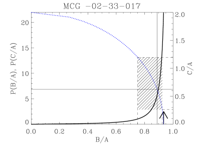
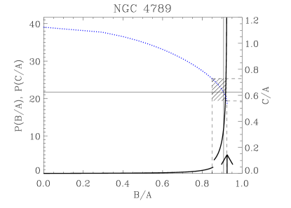
Figure 8: Relation between the axial ratios $B/A$ and $C/A$ for two sample bulges. MCG -02-33-017 (upper panel) hosts a bulge with $\phi_{M}<\phi_{C}$ and NGC 4789 (lower panel) hosts a bulge with $\phi_{M}>\phi_{C}$. The probability associated with each value of $B/A$ and its corresponding value of $C/A$ (thick solid line), the value of $C/A$ as a function of $B/A$ (dotted line), the maximum value of the equatorial ellipticity (arrow), the median values of $B/A$ (vertical thin solid line) and $C/A$ (horizontal thin solid line), and the confidence region which encloses all the possible values of $B/A$ and $C/A$ within a $67\%$ probability (hatched area) are shown in both panels.

5.1 Statistics of the intrinsic shape of bulges

Following the above prescriptions, we calculated the axial ratios $B/A$ and $C/A$ and their confidence intervals for all the sample bulges. There is no correlation between $B/A$ and $C/A$ (Fig. 9), unless only bulges with $\phi_{C}>\phi_{\rm M}$ are taken into account. The range of $C/A$ values corresponding to a given $B/A$ decreases as $B/A$ ranges from 1.0 to 0.5, giving a triangular shape to the distribution of allowed axial ratios. Circular and nearly circular bulges can have either an axisymmetric oblate or an axisymmetric prolate or a spherical shape. More elliptical bulges are more elongated along their polar axis.

Figure 9: The intrinsic shape of the 148 sample bulges. The axial ratios with $50\%$ probability are plotted for each bulge. Diamonds refer to the 115 sample bulges with $\phi_{C}>\phi_{\rm M}$.

We derived the triaxiality parameter, as defined by Franx et al. (1991), for the 115 sample bulges with a well-constrained intrinsic shape (i.e., those with $\phi_{C}>\phi_{\rm M}$)

$$T=\frac{1-\left(\frac{\hat{B}}{\hat{A}}\right)^{2}}{1-\left(\frac{\hat{C}}{\hat{A}}\right)^{2}},$$ (62)

where $\hat{A}$, $\hat{B}$, and $\hat{C}$ are the lengths of the longest, intermediate, and shortest semi-axes of the triaxial ellipsoid, respectively (i.e., $\hat{A}\geq\hat{B}\geq\hat{C}$). This notation is different with respect to that we adopted in the previous sections. Oblate triaxial (or axisymmetric) ellipsoids can be flattened either along the $y-$axis on the equatorial plane of the galaxy or along the polar axis. Prolate triaxial (or axisymmetric) ellipsoids can be elongated either along the $x-$axis on the equatorial plane of the galaxy or along the polar axis. Therefore, prolate bulges do either lie on the disk plane (and are similar to bars) or do stick out from the disk (and are elongated perpendicularly to it). This change of notation is needed to compare our results with those available in literature.

The triaxiality parameter for bulges with $\phi_{C}>\phi_{\rm M}$ is characterized by a bimodal distribution (Fig. 10) with a minimum at $T=0.55$ and two maxima at $T=0.05$ and $T=0.85$, respectively. According to this distribution, $65\%\pm 4\%$ of the selected bulges are oblate triaxial (or axisymmetric) ellipsoids ($T<0.55$) and the remaining $35\%\pm 4\%$ are prolate (or axisymmetric) triaxial ellipsoids ($T\geq 0.55$). The uncertainties for the percentages were estimated by means of Montecarlo simulations. Since $T$ is a function of $\phi$, we generated 10000 random values of $\phi$ in the range between $\phi_{B}$ and $\phi_{C}$ for each bulge and derived the corresponding distributions of $B/A$ and $C/A$ according to their PDFs. From $B/A$ and $C/A$ we calculated the distribution of $T$ and its standard deviation, which we adopted as uncertainty.

We investigated the cause of such a bimodality by separating the bulges according to their Sérsic index ($n$) and bulge-to-total luminosity ratio ($B/T$). Both quantities were derived for each sample bulge in Paper I. The Sérsic index is a shape parameter describing the curvature of the surface-brightness profile of the bulge. A profile with $n=1$ corresponds to an exponential law, while a profile with $n=4$ corresponds to an $r^{1/4}$ law. The bimodality is driven by bulges with Sérsic index $n>2$ (Fig. 10, upper panel), or alternatively, by bulges of galaxies with $B/T>0.3$ (Fig. 10, lower panel). In fact, the sample of bulges with $\phi_{C}>\phi_{\rm M}$ and the two subsamples of bulges with $n>2$ and of bulges in galaxies with $B/T>0.3$ are characterized by the same distribution of $T$, as confirmed at high confidence level ($>99\%$) by a Kolmogorov-Smirnov test. We find that $66\%\pm 4\%$ of bulges with $n>2$ have $T<0.55$. Their number decreases as $T$ increases from 0 to 0.55. The remaining bulges have $T>0.55$ and their number increases as $T$ ranges from 0.55 to 1. A similar distribution is observed for the bulges of galaxies with $B/T>0.3$. $67\%\pm 4\%$ of them host a bulge with $T<0.55$. Instead, the distribution of the triaxiality parameter of bulges of galaxies with $B/T\leq 0.3$ is almost constant with a peak at $T=0.05$. This is true also for the bulges with $n\leq 2$, although to a lesser degree.

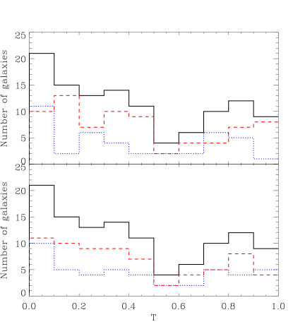
Figure 10: Distribution of the triaxiality parameter $T$ for the 115 bulges with $\phi_{C}>\phi_{\rm M}$ (continuous line). The distributions of bulges with Sérsic index $n\leq 2$ (dotted line) and $n>2$ (dashed line) are shown in the upper panel. The distributions of bulges of galaxies with bulge-to-total ratio $B/T\leq 0.3$ (dotted line) and $B/T>0.3$ (dashed line) are shown in the lower panel.

The two subsamples of bulges with $n\leq 2$ and $n>2$ are different, as confirmed by a Kolmogorov-Smirnov test ($99\%$ confidence level). In particular, the fraction of oblate axisymmetric (or nearly axisymmetric) bulges ($T<0.1$) is remarkably higher for $n\leq 2$ ($27\%\pm 4\%$) than for $n>2$ ($14\%\pm 3\%$). The fraction of triaxial bulges ($0.1\leq T\leq 0.9$) is lower for $n\leq 2$ ($71\%\pm 5\%$) than for $n>2$ ($76\%\pm 3\%$). The fraction of prolate axisymmetric (or nearly axisymmetric) bulges ($T>0.9$) for $n\leq 2$ is $2\%\pm 2\%$, but $11\%\pm 3\%$ for $n>2$.

The two subsamples of bulges of galaxies with $B/T>0.3$ and $B/T\leq 0.3$ are different too, as confirmed by a Kolmogorov-Smirnov test ($99\%$ confidence level). The fraction of oblate axisymmetric bulges ($T<0.1$) is significantly higher for bulges of galaxies with $B/T\leq 0.3$ ($22\%\pm 4\%$) than for $B/T>0.3$ ($16\%\pm 2\%$). The fraction of triaxial bulges ($0.1\leq T\leq 0.9$) is significantly lower for $B/T\leq 0.3$ ($67\%\pm 4\%$) than for $B/T>0.3$ ($78\%\pm 3\%$). A few prolate bulges ($T>0.9$) are observed for $B/T\leq 0.3$ ($11\%\pm 3\%$) and $B/T>0.3$ ($6\%\pm 2\%$). The distribution of bulges with $n\leq 2$ and bulges of galaxies with $B/T\leq 0.3$ appears to be the same at a high confidence level ($>99\%$) as confirmed by a Kolmogorov-Smirnov test.

Bulges with $\phi_{C}>\phi_{\rm M}$ can be divided into two classes: those with $n\leq 2$ (or $B/T\leq 0.3$) and those with $n>2$ (or $B/T>0.3$). About $70\%$ of bulges with $n\leq 2$ are hosted by galaxies with $B/T\leq 0.3$. The same is true for bulges with $n>2$ which are mostly hosted by galaxies with $B/T>0.3$. This agrees with the correlation between $n$ and $B/T$.

In order to understand whether the intrinsic shape is correlated with some of the bulge properties we measured in Paper I, we plotted the axial ratios $C/A$ and $B/A$ and the triaxiality of the sample bulges with $\phi_{C}>\phi_{\rm M}$ as a function of their Sérsic index, $J$-band luminosity, and central velocity dispersion (Fig. 11). As we found in Paper I for the intrinsic equatorial ellipticity, there are no statistically significant correlations between the bulge shape and the bulge Sérsic index, luminosity or velocity dispersion as pointed out by the low Spearman rank correlation coefficient (Fig. 11). However, this could be a selection effect since the sample of observed bulges spans over a limited range of Hubble types (S0–Sb).

Figure 11: The bulge axial ratios $C/A$ and $B/A$ and the triaxiality $T$ as a function of the bulge Sérsic parameter $n$, $J$-band luminosity $L_{\rm b}$ and central velocity dispersion $\sigma_{0}$. Only the 115 bulges with $\phi_{C}>\phi_{\rm M}$ are represented. The Spearman rank correlation coefficient ($\rho$) is shown in upper right corner of each panel.

5.2 The influence of nuclear bars on the intrinsic shape of bulges

Our sample galaxies were selected to not host large-scale bars. We checked for their presence in Paper I by a visual inspection of both the original image and the residual image we obtained after subtracting the best-fitting photometric model. However, these selection criteria did not account for the presence of unresolved nuclear bars. Nuclear bars are more elongated than their host bulges and have random orientations, therefore they could affect the measurement of the structural parameters of bulges and consequently of their intrinsic shape.

In Paper I we built up a set of 1000 artificial images with a Sérsic bulge, an exponential disk, and a Ferrers nuclear bar to study the effects of the bar on the measurements of the photometric parameters of bulge and disk. The mean errors on the fitted axial ratio and position angle of the bulge ($\langle\Delta q_{\rm b}\rangle$, $\langle\Delta{\rm PA}_{\rm b}\rangle$) and disk ($\langle\Delta q_{\rm d}\rangle$, $\langle\Delta{\rm PA}_{\rm d}\rangle$) and their standard deviations ($\delta\Delta q_{\rm b}$, $\delta\Delta{\rm PA}_{\rm b}$, $\delta\Delta q_{\rm d}$, $\delta\Delta{\rm PA}_{\rm d}$) are given in Table 2 of Paper I.

In the present paper, we tested whether including a nuclear bar affects the $T$ distribution. For each galaxy, we randomly generated a series of 1000 values of $q_{\rm b}$, $q_{\rm d}$, ${\rm PA}_{\rm b}$, and ${\rm PA}_{\rm d}$. To assess whether the bulges appear elongated and twisted with respect to the disk due to the presence of a nuclear bar, we assumed that the axial ratios were normally distributed around the values $q_{\rm b}+\langle\Delta q_{\rm b}\rangle$ and $q_{\rm d}+\langle\Delta q_{\rm d}\rangle$ with standard deviations $\delta\Delta q_{\rm b}$ and $\delta\Delta q_{\rm d}$, respectively, and that the position angles were normally distributed around the values ${\rm PA}_{\rm b}\pm\langle\Delta{\rm PA}_{\rm b}\rangle$ and ${\rm PA}_{\rm d}\pm\langle\Delta q_{\rm d}\rangle$ with standard deviations $\delta\Delta{\rm PA}_{\rm b}$ and $\delta\Delta{\rm PA}_{\rm d}$, respectively. We chose the PA values that gave the smallest $\delta$ with respect to the observed one.

If we assume that all the artificial bulges host a nuclear bar, we still obtain a bimodal distribution of $T$ (Fig. 12). However, the fraction of oblate axisymmetric (or nearly axisymmetric) bulges ($T<0.1$) is higher ($23\%\pm 2\%$) with respect to the observed $18\%\pm 3\%$. For a more realistic fraction of galaxies which host a nuclear bar (i.e, $30\%$, see Laine et al. 2002; Erwin 2004), the resulting distribution of $T$ is consistent within errors with the distribution derived in Sect. 5.1 (Fig. 12). We found that $20\%\pm 2\%$, $71\%\pm 3\%$, and $9\%\pm 2\%$ of the sample bulges are oblate axisymmetric ($T<0.1$), triaxial ($0.1\leq T\leq 0.9$), and prolate axisymmetric ($T>0.9$), respectively, with respect to the $18\%\pm 3\%$, $74\%\pm 4\%$, and $8\%\pm 2\%$ previously found. In addition, we have also tested the effects of not consider a distribution of bar parameters but only the stronger bar included in the simulations (0.8 $\times$ r_e, q_b = 0.2, and L_bar = 0.02 $\times$ L_tot), i.e., the worst-case scenario . If we assume that 30$\%$ of our galaxies host this kind of nuclear bars the results change strongly, obtaining that only $56\%\pm 4\%$ of the sample bulges are triaxial ($0.1\leq T\leq 0.9$) with respect to the $74\%\pm 4\%$ previously found. Considering that all galaxies host such kind of nuclear bars the fraction of triaxial bulges is $30\%\pm 3\%$.

The measured ellipticity and bulge misalignment with the disk of the artificial galaxies without a nuclear bar are smaller with respect to the actual values measured for the sample bulges. This sets an upper limit to the axisymmetry of the bulges.

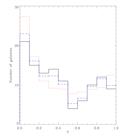
Figure 12: Distribution of the triaxiality parameter $T$ for the original sample of 115 bulges with $\phi_{C}>\phi_{\rm M}$ (continuous line), for a sample with $30\%$ of bulges with a nuclear bar (dashed line) and for a $100\%$ fraction of galaxies hosting a nuclear bar (dotted line).

6 Conclusions

In this work, we have developed a new method to derive the intrinsic shape of bulges. It is based upon the geometrical relationships between the observed and intrinsic shapes of bulges and their surrounding disks. We assumed that bulges are triaxial ellipsoids with semi-axes of length $A$ and $B$ in the equatorial plane and $C$ along the polar axis. The bulge shares the same center and polar axis of its disk, which is circular and lies on the equatorial plane of the bulge. The intrinsic shape of the bulge is recovered from photometric data only. They include the lengths $a$ and $b$ of the two semi-major axes of the ellipse, corresponding to the two-dimensional projection of the bulge, the twist angle $\delta$ between the bulge major axis and the galaxy line of nodes, and the galaxy inclination $\theta$. The method is completely independent of the studied class of objects, and it can be applied whenever a triaxial ellipsoid embedded in (or embedding) an axisymmetric component is considered.

We analyzed the magnitude-limited sample of 148 unbarred S0–Sb galaxies, for which we have derived (Paper I) the structural parameters of bulges and disks by a detailed photometric decomposition of their near-infrared surface-brightness distribution.

From the study of the equatorial ellipticity $Z=B^{2}/A^{2}$, we found that there is a combination of the characteristic angles for which the intrinsic shape can be more confidently constrained. This allowed us to select a qualified subsample of 115 galaxies with a narrow confidence interval (corresponding to $67\%$ of probability) of $Z$. For example, bulges with $B\approx A$ are among those characterized by the narrower confidence interval and the best determination of $Z$. The fraction of selected bulges with a maximum equatorial ellipticity $Z_{\rm M}<0.80$ ($B/A<0.89$), mean equatorial ellipticity $\langle Z\rangle<0.80$ and a median equatorial ellipticity $Z_{1/2}<0.80$ is $33\%$, $55\%$ and $43\%$, respectively. We conclude that not all the selected bulges have a circular (or nearly circular) section, but a significant fraction of them is characterized by an elliptical section. These bulges are strong candidates to be triaxial. In spite of the lower fraction of bulges with a maximum equatorial ellipticity smaller than 0.8, $Z_{\rm M}$ is a good proxy for the equatorial ellipticity because the selected sample contains all the bulges with $B\approx A$.

The analysis of the intrinsic flattening $F=2\,C^{2}/(A^{2}+B^{2})$ shows that only a few bulges of the selected sample are prolate triaxial ellipsoids. Only $22\%$ and $17\%$ have a mean intrinsic flattening $\langle F\rangle>1$ or a median intrinsic flattening $F_{1/2}>1$, respectively. The fraction rises to $90\%$ when a maximum intrinsic flattening $F_{\rm M}>1$ is considered. However, this is due to the projection effect of triaxial ellipsoids. Indeed, the fraction of bulges which are actually elongated along the polar axis is very small: only $18\%$ of bulges with $F_{\rm M}>1$ have a probability greater than $50\%$ to have an intrinsic flattening $F>1$, and there are no bulges with more than a $90\%$ probability of having $F>1$. Thus, $F_{\rm M}$ is not a good proxy for the intrinsic flattening.

After considering the equatorial ellipticity and intrinsic flattening as independent parameters, we derived the relation among them in order to calculate for each sample bulge both axial ratios, $B/A$ and $C/A$, and their confidence intervals. As already found for $Z$ and $F$, the axial ratios are better constrained for the selected sample of 115 bulges. We derived the triaxiality parameter, as defined by Franx et al. (1991), for all of them. We found that it follows a bimodal distribution with a minimum at $T=0.55$ and two maxima at $T=0.05$ (corresponding to oblate axisymmetric or nearly axisymmetric ellipsoids) and $T=0.85$ (strongly prolate triaxial ellipsoids), respectively. According to this distribution, $65\%$ of the selected bulges are oblate triaxial (or axisymmetric) ellipsoids ($T<0.55$) and the remaining $35\%$ are prolate triaxial (or axisymmetric) ellipsoids ($T>0.55$). This bimodality is driven by bulges with Sérsic index $n>2$ or alternatively by bulges of galaxies with a bulge-to-total ratio $B/T>0.3$. Bulges with $n\leq 2$ and bulges of galaxies with $B/T\leq 0.3$ follow a similar distribution, which is different from that of bulges with $n>2$ and bulges of galaxies with $B/T>0.3$. In particular, the sample of bulges with $n\leq 2$ and the sample of bulges of galaxies with $B/T\leq 0.3$ show a larger fraction of oblate axisymmetric (or nearly axisymmetric) bulges ($T<0.1$), a smaller fraction of triaxial bulges ($0.1\leq T\leq 0.9$), and fewer prolate axisymmetric (or nearly axisymmetric) bulges ($T>0.9$) with respect to the corresponding sample of bulges with $n>2$ and the sample of bulges of galaxies with $B/T>0.3$, respectively.

The different distribution of the intrinsic shapes of bulges according to their Sérsic index gives further support to the presence of two bulge populations with different structural properties: the classical bulges, which are characterized by $n>2$ and are similar to low-luminosity elliptical galaxies, and pseudobulges, with $n\leq 2$ and characterized by disk-like properties (see Kormendy & Kennicutt 2004, for a review). The correlation between the intrinsic shape of bulges with $n\leq 2$ and those in galaxies with $B/T\leq 0.3$ and between bulges with $n>2$ and those in galaxies with $B/T>0.3$ agrees with the correlation between the bulge Sérsic index and bulge-to-total ratio of the host galaxy, as recently found by Drory & Fisher (2007) and Fisher & Drory (2008).

No statistically significant correlations have been found between the intrinsic shape of bulges and bulge luminosity or velocity dispersion. However, this could be a selection effect since the sample bulges span a limited range of Hubble types (S0–Sb).

The observed bimodal distribution of the triaxiality parameter can be compared to the properties predicted by numerical simulations of spheroid formation. Cox et al. (2006) studied the structure of spheroidal remnants formed from major dissipationless and dissipational mergers of disk galaxies. Dissipationless remnants are triaxial with a tendency to be more prolate, whereas dissipational remnants are triaxial and tend be much closer to oblate. This result is consistent with previous studies of dissipationless and dissipational mergers (e.g., Barnes 1992; Hernquist 1992; Springel 2000; González-García & Balcells 2005). In addition, Hopkins et al. (2010) used semi-empirical models to predict galaxy merger rates and contributions to bulge growth as functions of merger mass, redshift, and mass ratio. They found that high $B/T$ systems tend to form in major mergers, whereas low $B/T$ systems tend to form from minor mergers. In this framework, bulges with $n\leq 2$, which shows a high fraction of oblate axisymmetric (or nearly axisymmetric) shapes and have $B/T\leq 0.3$, could be the result of dissipational minor mergers. A more complex scenario including both major dissipational and dissipationless mergers is required to explain the variety of intrinsic shapes found for bulges with $n>2$ and $B/T>0.3$.

On the other hand, depending on the initial conditions (see Vietri 1990, and references therein), the final shape of the early protogalaxies could also be triaxial. However, high-resolution numerical simulations in a cosmologically motivated framework that resolves the bulge structure are still lacking. The comparison of a larger sample of bulges with a measured intrinsic shape and covering the entire Hubble sequence with these numerical experiments is the next logical step in addressing the issue of bulge formation.