NUMERICAL SIMULATIONS OF THERMOHALINE CONVECTION: IMPLICATIONS FOR EXTRA-MIXING IN LOW-MASS RGB STARS

Abstract

Low-mass stars are known to experience extra-mixing in their radiative zones on the red-giant branch (RGB) above the bump luminosity. To determine if the salt-fingering transport of chemical composition driven by ³He burning is efficient enough to produce RGB extra-mixing, 2D numerical simulations of thermohaline convection for physical conditions corresponding to the RGB case have been carried out. We have found that the effective ratio of a salt-finger’s length to its diameter $a_{\rm eff}\lesssim 0.5$ is more than ten times smaller than the value needed to reproduce observations ($a_{\rm obs}\gtrsim 7$). On the other hand, using the thermohaline diffusion coefficient from linear stability analysis together with $a=a_{\rm obs}$ is able to describe the RGB extra-mixing at all metallicities so well that it is tempting to believe that it may represent the true mechanism. In view of these results, follow-up 3D numerical simulations of thermohaline convection for the RGB case are clearly needed.

1 Introduction

A main sequence (MS) star with a mass $M\lesssim 1.5\,M_{\odot}$, e.g. the Sun, gets its energy from thermonuclear fusion reactions of the pp-chains. When its core has exhausted the hydrogen fuel, the star leaves the MS and becomes a red giant branch (RGB) star. The red giant has a compact electron-degenerate helium core of the size of the Earth surrounded by a thin hydrogen burning shell (hereafter, HBS) that provides the star with the energy via the transformation of H into He via the CNO-cycle. The bulk of the red giant’s volume is occupied by a convective envelope that extends from the surface to nearly the HBS, however the base of the convective envelope always stays separated from the HBS by a convectively stable radiative zone with a thickness of the order of one solar radius.

It is possible to select a large sample of low-mass post-MS stars that have very similar masses and metallicities. The simplest way to do this is to choose normal post-MS stars belonging to a same several billion year old open or globular cluster. For field stars, one needs well-measured distances to estimate the masses accurately enough, so that only stars with well-determined Hipparcos parallaxes suit this purpose. A distribution of the characteristics of stars from such a sample along the RGB in the Hertzsprung-Russell (HR) diagram can then be interpreted as an evolutionary sequence (the Vogt-Russell theorem). In particular, a correlation of a surface chemical composition anomaly (a deviation of atmospheric abundances from those on the MS) with the luminosity or effective temperature can be considered as an evolutionary pattern produced by nuclear reactions and ongoing mixing.

Spectroscopic observations and their theoretical interpretations have firmly established two distinct mixing episodes in low-mass RGB stars (e.g., Charbonnel 1994). First, on the lower RGB, the convective envelope quickly grows in mass and, as a result, its base penetrates the layers in which the partial burning of H via the pp-chains resulted in an accumulation of large amounts of ³He, and where Li was mostly destroyed. It also reaches the layers in which the non-equilibrium operation of the CN-branch of the CNO-cycle took place. This should lead to sharp changes of the star’s atmospheric chemical composition, such as a strong decrease of its surface Li abundance, a noticeable reduction of the ¹²C/¹³C isotopic ratio, a modest decrease and increase of the C and N abundances respectively, and a considerable enrichment of the convective envelope in ³He. These changes continue until the convective envelope attains its maximum mass after which its base starts to recede in front of the HBS advancing in mass. This mixing episode is called the first dredge-up. All of the above predicted changes of the star’s surface chemical composition, except those of ³He, have often been observed on the lower RGB.

Second, on the upper RGB, above the luminosity at which differential luminosity functions of globular-cluster RGB stars have clearly visible bumps, observations reveal that the same abundance changes that were occurring during the first dredge-up resume, and that the changes are even larger this time. The bump luminosity corresponds to the evolutionary phase during which the HBS passes through and erases the chemical composition discontinuity imprinted by the convective envelope at the end of the first dredge-up. When the HBS crosses the discontinuity it finds itself in a region with a slightly increased H abundance; consequently, the red giant readjusts its structure appropriately, causing it to move to slightly lower luminosities before continuing up the RGB. As a result of spending more time in the narrow range of luminosity where this readjustment occurs, there is a pile-up of stars around the bump luminosity. Given that the base of convective envelope recedes through a region of homogeneous chemical composition, the observed evolutionary variations of the surface abundances on the upper RGB can be understood only if there is some extra-mixing process of non-convective origin that connects the convective envelope with the HBS. The physical nature of this extra-mixing still remains elusive. For a long time, it has been thought that the RGB extra-mixing is related to rotation-induced instabilities (e.g., Sweigart & Mengel 1979; Charbonnel 1995; Denissenkov & Tout 2000). However, the work of Palacios et al. (2006) casts doubt on these models.

It was not until recently that the most promising mechanism of the RGB extra-mixing was proposed by Eggleton, Dearborn, & Lattanzio (2006) and Charbonnel & Zahn (2007). When the HBS is approached from the base of convective envelope, the first active thermonuclear reaction involving abundant nuclei that is encountered is ³He(³He,2p)⁴He. It has a unique property of lowering the mean molecular weight locally, by $\Delta\mu\approx\mu^{2}\Delta X(^{3}\mbox{He})/6$, where $\Delta X(^{3}\mbox{He})$ is a mass fraction of ³He consumed in the reaction. As a consequence, the density is reduced by the same amount (assuming the ideal gas law), which makes the local material lighter than that in its immediate surroundings, therefore the ³He-depleted material will tend to rise. Mixing driven by ³He burning in stars was discussed already in the 1970s (e.g., Ulrich 1972), however it was the publication by Eggleton, Dearborn, & Lattanzio (2006) that brought this mechanism to the attention of other researchers in the context of the RGB extra-mixing.

Charbonnel & Zahn (2007) have given a correct physical explanation of the mixing process to which the ³He burning in the HBS should lead. This is the salt-fingering or thermohaline convection that has been studied in detail, both experimentally and theoretically, in oceanography for many years (e.g., see reviews by Ruddick & Kerr 2003, Schmitt 2003, and Kunze 2003). It is caused by a double-diffusive instability that occurs in a situation when a stabilizing agent (heat) diffuses away faster than a destabilizing agent (salt and $\mu$ in the oceanic and RGB cases, respectively). In the ocean, the double-diffusive instability usually develops close to the surface where warm salty water finds itself overlying cold fresh water. A blob of the surface water will tend to sink because its higher salinity (a concentration of salt) makes it denser than the surrounding deeper water while its temperature remains close to the ambient one thanks to the faster diffusion of heat. Similarly, a blob at depth will tend to rise. In the oceanic case, the usual outcome of this instability are vertically elongated salt fingers containing sinking and rising water of different salinity.

Given that the local reduction of $\mu$ by the ³He burning is very small, $\Delta\mu/\mu\sim-10^{-4}$, it can become visible only in the background of homogeneous chemical composition. This happens precisely at the bump luminosity. Another feature that makes the ³He-driven thermohaline convection the most promising mechanism for the RGB extra-mixing is its dependence on just one parameter, the envelope ³He abundance after the first dredge-up. This means that stars with similar masses and metallicities should demonstrate comparable chemical composition anomalies on the upper RGB, the pattern that seems to be observed in real stars (e.g., Gratton et al. 2000; Smith & Martell 2003). Before the RGB extra-mixing was introduced into the standard stellar evolution theory, the latter had been in conflict with the seemingly observed constancy of the interstellar ³He abundance since the Big Bang. The problem is that low-mass stars produce a lot of ³He on the MS that is dredged up to the surface on the RGB and then deposited in the interstellar medium as a result of mass-loss. The most plausible solution of this problem is the RGB extra-mixing that strongly decreases the envelope abundance of ³He by circulating it through the ³He burning layers of the HBS. Therefore, if the RGB extra-mixing is indeed driven by the ³He burning (thermohaline convection) then the cosmological ³He problem has a beautiful solution: it is ³He itself abundantly produced in low-mass MS stars that takes care of its own destruction in the same stars on the RGB, so that the net balance of ³He from low-mass stars in the interstellar medium is close to zero.

Charbonnel & Zahn (2007) have modeled thermohaline mixing using a diffusion coefficient obtained from a linear theory by Ulrich (1972). Unfortunately, the linear theory does not give a reliable estimate of the maximum length of salt fingers relative to their diameter, i.e., the finger aspect ratio $a=l/d$, the square of which enters the diffusion coefficient. This leads to a large uncertainty in the theory leaving it basically semi-empirical, like other up-to-date theories and models of the RGB extra-mixing. From the results presented by Charbonnel & Zahn (2007), it follows that the surface abundance patterns in low-mass RGB stars can be reproduced theoretically only if $a\gg 1$. To support the large finger aspect ratio, Charbonnel & Zahn (2007) referred to the oceanic case where long salt fingers were observed experimentally. However, it is not legitimate to directly compare the oceanic and RGB cases because they correspond to very different fluid flows sets. In particular, the ratio of viscosity to thermal diffusivity (the Prandtl number $Pr$) is close to ten for the oceanic case, whereas $Pr<10^{-5}$ for the RGB case. It turns out that only direct numerical simulations with non-linear interactions and other relevant effects taken into account can give better insight into the ³He-driven thermohaline mixing in the low-mass RGB stars. It is this task that is addressed in this research for the first time.

The paper is organized as follows. Section 2 summarizes the main results from the linear theory that are relevant for our further discussion. Section 3 presents and analyzes the results of our 2D numerical simulations of thermohaline convection. It is followed by Section 4, in which we employ a diffusion coefficient from the linear theory to model, as precisely as possible, the changes of chemical composition incurred by the RGB thermohaline mixing. Discussion and conclusions are provided in the final Section 5. Wherever it is appropriate, we make a comparison of the oceanic and RGB cases.

2 Relevant Results from the Linear Salt-Fingering Theory

In this as well as in the next section, our analysis begins with the Boussinesq equations that describe motion in a nearly incompressible stratified viscous fluid

$$\frac{\partial\mathbf{v}}{\partial t}+(\mathbf{v},\nabla)\mathbf{v} = \frac{\delta\rho}{\rho_{0}}\,\mathbf{g}+\nu\nabla^{2}\mathbf{v},$$ (1)

$$\frac{\partial T}{\partial t}+(\mathbf{v},\nabla)T = k_{T}\nabla^{2}T,$$ (2)

$$\frac{\partial S}{\partial t}+(\mathbf{v},\nabla)S = k_{S}\nabla^{2}S,$$ (3)

where $\mathbf{v}$ is the velocity, $\rho_{0}$ is a constant reference density, $\delta\rho$ is a deviation of the local density from $\rho_{0}$, $\mathbf{g}$ is the gravitational acceleration, $\nu$ is the viscosity, $T$ is the temperature, $S$ is the salinity, $k_{T}$ and $k_{S}$ are the thermal and haline diffusivities. Note that, in the RGB case, $S$ should be replaced by $\mu$, while equation (3) is still valid as long as $|\Delta\mu|/\mu\ll 1$. We have also neglected source terms in equations (2) and (3) that could be related to nuclear reactions in the RGB case.

In the Boussinesq approximation, which is a reasonable one even for a compressible fluid provided that its motion is studied on length scales much less than the density height scale and velocities remain much less than the speed of sound, the density variation is taken into account only in the buoyancy force term $\mathbf{f}_{\rm b}=(\delta\rho/\rho_{0})\,\mathbf{g}$. Assuming that the relative deviations of $\rho$, $T$, and $S$ from their reference values in the initial unperturbed state $(\rho_{0},T_{0},S_{0})$ are small, we use a linearized equation of state

$$\delta\rho=-\alpha\delta T+\beta\delta S,$$ (4)

where

$$\alpha=-\frac{1}{T}\left(\frac{\partial\ln\rho}{\partial\ln T}\right)_{P},\ \ \ \mbox{and}\ \ \ \beta=\frac{1}{S}\left(\frac{\partial\ln\rho}{\partial\ln S}\right)_{P}$$

are the coefficients of thermal expansion and haline contraction. For the ideal gas law, which provides a good approximation to the equation of state in the radiative zone of a low-mass RGB star, we simply have $\alpha=1/T$ and $\beta=1/\mu$.

We use the Cartesian coordinate system $(x,y,z)$ oriented so that its vertical axis $z$ has a direction opposite to that of the gravitational acceleration and the $x$-axis is located in a star’s meridional plane. Let $w$ denote the velocity’s vertical component. Linearizing equations (1 – 3), we arrive at the following system of linear PDEs for the vertical velocity component and variations of temperature and salinity:

$$\frac{\partial w}{\partial t} = g(\alpha\delta T-\beta\delta S)+\nu\nabla^{2}w,$$ (5)

$$\frac{\partial\delta T}{\partial t} = -w\frac{\partial T}{\partial z}+k_{T}\nabla^{2}\delta T,$$ (6)

$$\frac{\partial\delta S}{\partial t} = -w\frac{\partial S}{\partial z}+k_{S}\nabla^{2}\delta S.$$ (7)

Given that we seek a solution representing vertically elongated structures with a large ratio of the vertical to horizontal length scales, we can neglect horizontal velocity components and we can also assume that $\nabla^{2}\approx\partial^{2}/\partial^{2}x+\partial^{2}/\partial^{2}y$.

Following Kunze (1987), we will take into consideration the influence of salt-fingering on the ambient temperature and salinity gradients that appear on the right-hand sides of equations (6) and (7). This influence is determined by the ratios $\delta_{T}=-2\delta T/\Delta T$ and $\delta_{S}=-2\delta S/\Delta S$, in which $\Delta T=(\partial T_{0}/\partial z)\,l$ and $\Delta S=(\partial S_{0}/\partial z)\,l$ are differences in temperature and salinity between two points separated by the finger length $l$ in the vertical direction in the initial unperturbed state. The factor of two in the above relations takes account of the fact that every sinking finger with excesses of S and T has a neighbouring rising finger possessing deficiencies of S and T of same magnitudes. The perturbed gradients are expressed via the new independent variables

$$\frac{\partial T}{\partial z}=\frac{\partial T_{0}}{\partial z}\,(1-\delta_{T}),$$ (8)

$$\frac{\partial S}{\partial z}=\frac{\partial S_{0}}{\partial z}\,(1-\delta_{S}),$$ (9)

where $0\leq(\delta_{T},\,\delta_{S})\leq 1$. With regard to the temperature gradient, it is important to note a difference between the oceanic and RGB cases. In the RGB case, one should subtract the adiabatic temperature gradient $(\partial T/\partial z)_{\rm ad}$ from both $\partial T/\partial z$ and $\partial T_{0}/\partial z$ in equation (8) because a temperature gradient is always negative in stars and it remains stable only as long as its absolute magnitude is less than that of the adiabatic gradient. The maximum effect that a salt-fingering heat flux can produce on $\partial T/\partial z$ is to render it adiabatic ($\delta_{T}=1$). In the oceanic case, any positive temperature gradient stabilizes the density stratification.

Finally, expressing $\delta T$ and $\delta S$ by $\delta_{T}$ and $\delta_{S}$ and substituting them into the system (5 – 7) gives

$$\frac{\partial w}{\partial t}-\nu\nabla^{2}w = \frac{l}{2}\,g\beta\,\frac{\partial S_{0}}{\partial z}\,(\delta_{S}-R_{\rho}\delta_{T}),$$ (10)

$$\frac{\partial\delta_{T}}{\partial t}-k_{T}\nabla^{2}\delta_{T} = \frac{2}{l}\,w\,(1-\delta_{T}),$$ (11)

$$\frac{\partial\delta_{S}}{\partial t}-k_{S}\nabla^{2}\delta_{S} = \frac{2}{l}\,w\,(1-\delta_{S}),$$ (12)

where $R_{\rho}=\alpha\Delta T/\beta\Delta S$ is a parameter known as the density ratio in oceanography. In stellar physics, it corresponds to $R_{\rho}=(\nabla-\nabla_{\rm ad})/\nabla_{\mu}$, where $\nabla=(\partial\ln T_{0}/\partial\ln P)$, $\nabla_{\rm ad}=(\partial\ln T/\partial\ln P)_{\rm ad}$, and $\nabla_{\mu}=(\partial\ln\mu_{0}/\partial\ln P)$. Solutions of the last equations are sought in the usual form of $w$, $\delta_{T}$, $\delta_{S}\propto\exp(\sigma t)\times\exp[\,i(k_{x}x+k_{y}y)]$ taking into account that the vertical velocity can be approximated as $w\approx\sigma l/2$, where $\sigma$ is the growth rate of salt fingers, whereas $k_{x}$ and $k_{y}$ are their horizontal wave numbers. After some simple algebra, the three equations are reduced to the following third-order dispersion relationship:

$$4\sigma^{3}+2(k_{T}+k_{S}+2\nu)k^{2}\sigma^{2}+\{[k_{T}k_{S}+2\nu(k_{T}+k_{S})]k^{4}+$$

$$2g\beta\,\frac{\partial S_{0}}{\partial z}\,(R_{\rho}-1)\}\sigma-g\beta\,\frac{\partial S_{0}}{\partial z}\,(k_{T}-R_{\rho}k_{S})k^{2}=0,$$ (13)

where $k=\sqrt{k_{x}^{2}+k_{y}^{2}}$ is related to the salt-finger diameter $d=2\pi/k$.

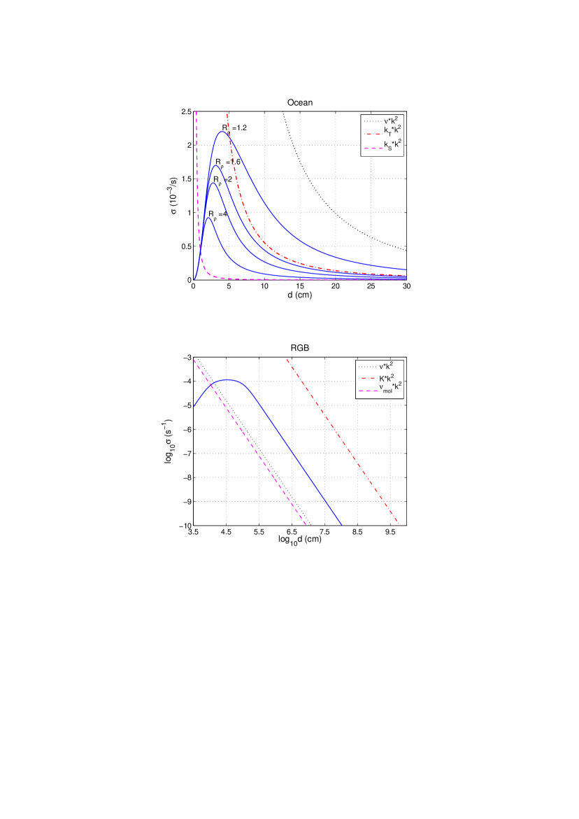
Figure 1: Solid curves show growth rates for salt fingers of different diameters for the oceanic (upper panel) and RGB (lower panel) cases. Dotted, dot-dashed and dashed curves are reciprocals of microscopic viscous, thermal and mixing timescales for perturbations with the wave number $k=2\pi/d$.

Positive real roots of equation (13), corresponding to exponentially growing solutions (the double-diffusive instability), are plotted in Fig. 1 for the oceanic (upper panel) and RGB (lower panel) cases. Note that, from here on, we will be using more customary notations for the stellar structure parameters related to salt-fingering, whereas those introduced so far will be reserved for the oceanic case. In particular, the thermal and haline diffusivities become the radiative and molecular diffusivities in the RGB case

$$k_{T} \rightarrow K=\frac{4acT^{3}}{3\varkappa C_{P}\rho^{2}},$$

$$k_{S} \rightarrow \nu_{\rm mol}=1.84\times 10^{-17}(1+7X)\,\frac{T^{5/2}}{\rho}\ (\mbox{cm}^{2}\,\mbox{s}^{-1}),$$

where $a$ is the radiation constant, $c$ is the speed of light, $\varkappa$ is the Rosseland mean opacity, $C_{P}$ is the specific heat at constant pressure, and $X$ is the hydrogen mass fraction. The viscosity in the vicinity of the HBS consists of comparable parts of $\nu_{\rm mol}$ and the radiative viscosity

$$\nu=\nu_{\rm mol}+\nu_{\rm rad},\ \ \mbox{where}\ \ \nu_{\rm rad}=\frac{4aT^{4}}{15c\varkappa\rho^{2}}.$$

For the reader’s convenience, Table 1 shows the correspondence between similar parameters in the oceanic and RGB cases as well as their characteristic values. For the oceanic case, we have used the data compiled by Kunze (1987) (also, see Table 1 in the review by Kunze 2003). For the RGB case, the data are taken from our bump luminosity model that has a mass $M=0.83\,M_{\odot}$ and heavy-element mass fraction $Z=0.0005$. They refer to a point in the ³He-burning region of the HBS shell at which $\nabla_{\mu}$ is negative and has its maximum absolute value (for model details, see Section 3.3).

From the lower panel of Fig. 1, it is seen that $Kk^{2}\gg 2\sigma$ and $Kk^{2}\gg 2\nu k^{2}\sim\nu_{\rm mol}k^{2}$ in the RGB case. This allows one to approximate the cubic equation (13) by the quadratic

$$2Kk^{2}\sigma^{2}+\left[K(2\nu+\nu_{\rm mol})k^{4}+2g\beta\frac{\partial\mu_{0}}{\partial z}(R_{\rho}-1)\right]\sigma$$

$$-g\beta\frac{\partial\mu_{0}}{\partial z}(K-R_{\rho}\nu_{\rm mol})k^{2}+\nu K\nu_{\rm mol}k^{6}=0.$$ (14)

For short horizontal wave numbers, such that

$$k^{4}\ll g\beta\frac{\partial\mu_{0}}{\partial z}\frac{(K-R_{\rho}\nu_{\rm mol})}{\nu K\nu_{\rm mol}},\ \ \mbox{and}\ \ k^{4}\ll 2g\beta\frac{\partial\mu_{0}}{\partial z}\frac{(R_{\rho}-1)}{K(2\nu+\nu_{\rm mol})},$$

a positive solution of (14) is simplified to

$$\sigma\approx\frac{1}{2}\,\frac{(K-R_{\rho}\nu_{\rm mol})}{(R_{\rho}-1)}\,k^{2}=2\pi^{2}\,\frac{(K-R_{\rho}\nu_{\rm mol})}{(R_{\rho}-1)}\,\frac{1}{d^{2}}.$$

The last expression describes very well the decline of the finger’s growth rate with an increase of its diameter at $d\gg d_{\rm max}=d(\sigma_{\rm max})$. It can be used to estimate a thermohaline diffusion coefficient $D_{\mu}\approx wl\approx\frac{1}{2}\sigma l^{2}$. This leads to the well-known results

$$D_{\mu}\approx\frac{1}{4}\,\frac{(K-R_{\rho}\nu_{\rm mol})}{R_{\rho}-1}\,k^{2}l^{2}=C\frac{\nabla_{\mu}}{\nabla_{\rm rad}-\nabla_{\rm ad}-\nabla_{\mu}}\left(1-\frac{\nu_{\rm mol}}{K}\,\frac{\nabla_{\rm rad}-\nabla_{\rm ad}}{\nabla_{\mu}}\right)\,a^{2}K,$$ (15)

where $C=C_{\rm Kunze}=\pi^{2}$ and

$$\nabla_{\rm rad}=\left(\frac{\partial\ln T_{0}}{\partial\ln P}\right)=\frac{3}{16\pi Gac}\,\frac{\varkappa P}{T^{4}}\,\frac{L_{r}}{M_{r}}$$

is the radiative temperature gradient, $M_{r}$ and $L_{r}$ being the mass and luminosity at the radius $r$ in the star (assuming spherical symmetry). The first of the expressions (15) indicates that the double-diffusive instability develops only when $1<R_{\rho}<1/\tau$, where $\tau=\nu_{\rm mol}/K=k_{S}/k_{T}$ is the inverse Lewis number. This result is known since the pioneering work of Stern (1960). Its discussion in regard to the RGB thermohaline mixing has been presented by Denissenkov & Pinsonneault (2008b) (also, see Vauclair 2004). Ulrich (1972), who neglected the influence of salt-fingering on the ambient $T$- and $\mu$-gradients, had obtained an expression for $D_{\mu}$ with the constant $C=C_{\rm Ulrich}=8\pi^{2}/3$. He did not retain the impeding factor in the parentheses either. It is Ulrich’s formula that has been employed by Charbonnel & Zahn (2007). Kippenhahn et al. (1980) used a different physical approach to arrive at a similar expression for $D_{\mu}$ with $C=C_{\rm Kipp}=12$. In addition, they came to the conclusion that, because of their strong interactions with the surrounding medium, the perturbed blobs of fluid did not have a chance to become salt-fingers, so that their aspect ratio should be as small as $a=l/d\approx 0.5$.

It is useful to estimate the diameter of the fastest growing fingers $d_{\rm max}$ as a function of other parameters. This can be done by analyzing the dependence of the positive root of equation (14) on the wave number $k$. It turns out that a sufficiently good approximation for both the oceanic and RGB cases is

$$d_{\rm max}\approx 2\pi\sqrt[4]{\frac{\nu k_{T}}{N_{T}^{2}}},$$ (16)

where $N_{T}^{2}$ is the square of the unperturbed $T$-component of the Brunt-Väisälä (buoyancy) frequency. For the RGB case, we have $N_{T}^{2}=(\nabla_{\rm ad}-\nabla_{\rm rad})g/H_{P}$, $H_{P}$ being the pressure scale height. We find that $N_{T}^{2}\approx 1.5\times 10^{-4}$ s^-2 at the same location in our RGB model for which the other data are listed in Table 1. Its substitution into (16) together with the values of $\nu$ and $k_{T}=K$ gives $\log_{10}d_{\rm max}\approx 4.4$ which is very close to the position of the maximum on the solid curve in the lower panel of Fig. 1.

Solid curves in Fig. 1 demonstrate that the diameter and velocity of the fastest growing salt fingers in the oceanic ($R_{\rho}=1.6$) and RGB cases are $d_{\rm max}^{\rm\,Ocean}\approx 3$ cm, $w_{\rm max}^{\rm Ocean}\approx 0.003\,a_{\rm max}^{\rm Ocean}$ cm s^-1, and $d_{\rm max}^{\rm RGB}\approx 0.3$ km, $w_{\rm max}^{\rm RGB}\approx 2\,a_{\rm max}^{\rm RGB}$ cm s^-1, where $a_{\rm max}^{\rm Ocean}$ and $a_{\rm max}^{\rm RGB}$ are the (unknown) finger aspect ratios for the corresponding cases. The major uncertainty in the linear theory is the parameter $a$. Its value can be estimated only by numerical simulations that directly solve the original non-linear equations (1 – 3). The double-diffusive instability is a primary instability. It is responsible for the initial growth of salt fingers. What will happen later on and, in particular, how far the fluid blob will travel vertically, forming a salt finger before its trajectory is bent or the finger gets destroyed by its interactions with other fingers and surrounding medium, is determined by secondary instabilities. It is this problem that we are going to address in the next section.

3 2D Numerical Simulations of Thermohaline Convection

3.1 Basic Equations and a Method of Their Solution

In the Boussinesq approximation, the continuity equation is simplified to $(\nabla,\mathbf{v})=0$. It can be automatically satisfied by representing the velocity vector with a stream function $\psi$, such that

$$\mathbf{v}=(u,w)=(-\frac{\partial\psi}{\partial z},\,\frac{\partial\psi}{\partial x}),$$ (17)

where $u$ is the velocity (horizontal) $x$-component. After the substitution of (17) into the original system (1 – 3), we obtain a new system of Boussinesq equations that contain only scalar functions and their derivatives

$$\frac{\partial\,\nabla^{2}\psi}{\partial t} = -J(\psi,\nabla^{2}\psi)+Pr\frac{\partial}{\partial x}(T^{\prime}-\frac{S^{\prime}}{R_{\rho}})+Pr\nabla^{4}\psi,$$ (18)

$$\frac{\partial T^{\prime}}{\partial t} = -J(\psi,T^{\prime})-\frac{\partial\psi}{\partial x}+\nabla^{2}T^{\prime},$$ (19)

$$\frac{\partial S^{\prime}}{\partial t} = -J(\psi,S^{\prime})-\frac{\partial\psi}{\partial x}+\tau\nabla^{2}S^{\prime},$$ (20)

where $J(a,b)=\frac{\partial a}{\partial x}\frac{\partial b}{\partial z}-\frac{\partial a}{\partial z}\frac{\partial b}{\partial z}$ is the Jacobian. Unlike the quantities $\delta T(x,y,t)$ and $\delta S(x,y,t)$ in equations (5 – 7), the variances $T^{\prime}$ and $S^{\prime}$ describe deviations of temperature and salinity from $T_{0}(z)$ and $S_{0}(z)$ not only in the horizontal plane but also along the radius, so that

$$T(x,z,t)=T_{0}(0)+\left(\frac{\partial T_{0}}{\partial z}\right)\,z+T^{\prime}(x,z,t),$$

$$S(x,z,t)=S_{0}(0)+\left(\frac{\partial S_{0}}{\partial z}\right)\,z+S^{\prime}(x,z,t),$$

where $T_{0}(0)$ and $S_{0}(0)$ are constants measuring the temperature and salinity in the initial unperturbed state at an arbitrarily chosen vertical position that corresponds to $z=0$. Equations (18 – 20) have been non-dimensionalized using $d$ and $d^{2}/k_{T}$ as the length and time units, where $d=d_{\rm max}/2\pi$, and dividing $T$ and $S$ by $(\partial T_{0}/\partial z)\,d$ and $(\partial S_{0}/\partial z)\,d$, respectively.

We solve the system of equations (18 – 20) numerically for a 2D doubly-periodic Cartesian domain by employing a computer code kindly provided by Bill Merryfield. According to him, the code uses a Fourier collocation method with dealiasing that follows the $2/3$ rule (Canuto et al. 1988). Integration in time is via the leapfrog method, with the time-splitting instability damped by applying a Robert filter with the parameter $0.002$ (e.g., Whitfield, Holloway, & Holyer 1989). Dissipation terms are represented by exponential integration factors. The linear portion of the code was tested by comparing the evolution of small initial perturbations to predictions of linear stability theory (Schmitt 1979). To check the non-linear portion, the code was tested for conservation of temperature variance, salinity variance, energy and enstrophy after the dissipation, buoyancy, and background gradient terms had been removed. Initial $S^{\prime}$ is specified by selecting Fourier coefficients from a bi-Gaussian distribution and scaling by $k^{-2}$, where $k$ is the magnitude of wave vector $\mathbf{k}$. The variance of initial non-dimensional $S^{\prime}$ is normalized to $0.1$. Initial values of $T^{\prime}$ and $\psi$ are set to zero.

3.2 The Oceanic Case

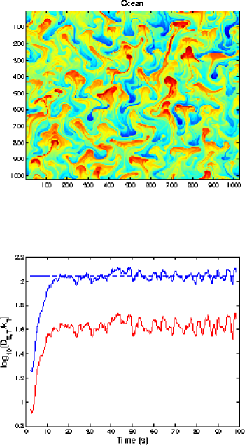
Figure 2: A snapshot of our $1024\times 1024$ numerical simulations of the oceanic salt-fingering at the equilibrium state (upper panel). A change of color from blue to red corresponds to an increase of salinity. Blue and red curves in the lower panel show the diffusion coefficients for the salinity and heat salt-fingering transport in units of the microscopic thermal diffusivity. The blue dashed line approximates the equilibrium value of $D_{S}/k_{T}$.

For test purposes, we have first reproduced one of the results presented by Merryfiled & Grinder (2000) in their unpublished paper (personal communication from Bill Merryfield). It corresponds to the oceanic case with the density ratio $R_{\rho}=1.6$ (Table 1). As output, the code directly gives the effective fingering salt and heat diffusivities, $D_{S}$ (denoted as $D_{\mu}$ in the RGB case) and $D_{T}$, normalized by $k_{T}$ ($K$). This is achieved by a procedure that first determines the fingering salt ($\mu$) and heat fluxes by spatially and temporally averaging the products $wS$ and $wT$ and then dividing them by $\partial S_{0}/\partial z$ ($\partial\mu_{0}/\partial z$) and $\partial T_{0}/\partial z$, respectively, after the fingers have attained statistical equilibrium. The horizontal size of the solution domain is initially chosen to be wide enough, $L_{x}=L_{z}=16\,d_{\rm max}$, so that the averaging does not produce large-amplitude fluctuations. The blue and red solid curves in the lower panel of Fig. 2 show transitions of the ratios $D_{S}/k_{T}$ and $D_{T}/k_{T}$ to their equilibrium values. The upper panel gives a snapshot of salt fingers in the statistical equilibrium. This solution has been obtained with a $1024\times 1024$ resolution for the salinity, while the code always uses a $2\times 2$ times lower resolution for $T$ and $\psi$. The dashed blue line in the lower panel plots the constant $D_{S}/k_{T}=2\pi^{2}a^{2}/R_{\rho}$, where $a=3$. It approximates the linear thermohaline diffusion coefficient (15) for $C=2C_{\rm Kunze}=2\pi^{2}=19.7$, given that $\tau\ll 1$ (Table 1). Here, as well as in the next section, we will compare our numerical results for $D_{S}$ and $D_{\mu}$ with those predicted by the linear theory (eq. 15) using $C=2C_{\rm Kunze}$. With this choice, $C$ lies approximately in the middle between $C_{\rm Kipp}=12$ and $C_{\rm Ulrich}=8\pi^{2}/3=26.3$. The comparison gives an effective value of the finger aspect ratio that, after being substituted in (15), leads to a value of the linear diffusion coefficient of the same order of magnitude as the one derived from our numerical simulations. In particular, we have obtained $a\approx 3$ for the test case. This estimate, as well as the salinity patterns in the upper panel of Fig. 2, confirm that we really deal with (i.e., reproduce numerically) vertically elongated structures (fingers) in the oceanic case.

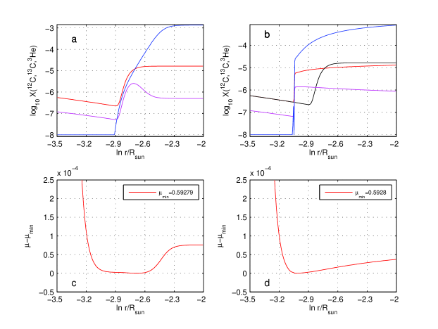
Figure 9: Same as in Fig. 5 but for the bump luminosity model with $Z=0.0001$ and $M=0.85\,M_{\odot}$.

Note that, although not perfect, the 2D numerical simulations of salt-fingering in the ocean have succeeded in producing both the salt and heat fluxes compatible with those measured by St. Laurent & Schmitt (1999) in the North Atlantic tracer release experiment (e.g., Fig. 9 in the review by Kunze 2003).

3.3 The RGB Case

We have employed two stellar evolution codes to compute bump luminosity models of low-mass RGB stars: our own code, the most recent version of which is described by Denissenkov et al. (2010), and the MESA code available at http://mesa.sourceforge.net. The combinations of mass, heavy-element and helium mass fractions for which the models have been computed with our code are $(M/M_{\odot},Z,Y)=(0.83,0.0005,0.24),\ (0.83,0.001,0.24)$, and $(0.83,0.002,0.24)$, while the models produced with the MESA code have $(M/M_{\odot},Z,Y)=(0.85,0.0001,0.24),\ (0.83,0.001,0.24)$, and $(1.5,0.0188,0.27)$. The MESA lowest-metallicity model reproduces conditions at which the RGB extra-mixing is thought to be most efficient, according to both observations and theory (e.g., Martell, Smith, & Briley 2008). The parameters of the common model, $M=0.83\,M_{\odot}$ and $Z=0.001$, are close to those of the field stars with known Hipparcos parallaxes for which evolutionary abundance changes have been found on the upper RGB by Gratton et al. (2000). Finally, the solar-metallicity model has a mass and composition typical for the so-called Li-rich giants that are located close to the bump luminosity (Charbonnel & Balachandran 2000) and in which Li is believed to be produced in a large amount by enhanced extra-mixing (Denissenkov & Herwig 2004).

Sharp declines of both the Li abundance and carbon isotopic ratio at the bump luminosity in the majority of low-mass RGB stars (e.g., Gratton et al. 2000; Shetrone 2003; D’Orazi & Marino 2010) demonstrate that the RGB extra-mixing starts to operate and becomes very efficient already at this evolutionary phase. Hence, if it is actually caused by the ³He burning and its associated thermohaline convection, the latter should already be present in the bump luminosity models in which the HBS has erased the chemical composition discontinuity left behind by the base of convective envelope at the end of the first dredge-up and, as a result, the $\mu$ depression produced by the ³He burning is now a prominent feature on the otherwise uniform $\mu$ profile outside the HBS.

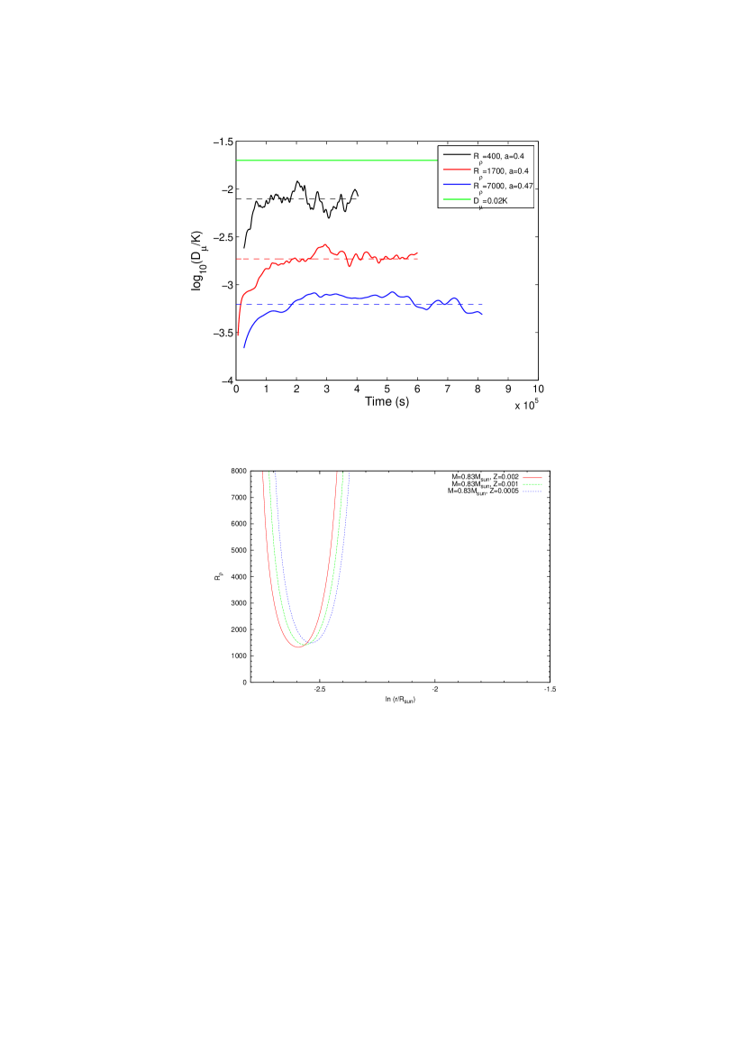
Figure 3: Upper panel shows thermohaline diffusion coefficients (oscillating curves) and their corresponding equilibrium values (dashed lines) obtained in our 2D numerical simulations for the density ratios $R_{\rho}=400$, 1700, and 7000, which are close to those found in the radiative zones of RGB stars (lower panel). The solid green line in the upper panel gives the empirically constrained rate of the RGB extra-mixing. The diffusion coefficients are divided by the thermal diffusivity. In the upper panel, the inset also shows the effective finger aspect ratios ($a$) that produce the corresponding equilibrium values (dashed lines) when $C=2C_{\rm Kunze}=2\pi^{2}$ is substituted in the expression (15).

MESA is a state-of-the-art stellar evolution code that even allows non-stop computations through the helium core flash toward the end of the asymptotic giant branch (AGB) evolution for low-mass stars. We will use the MESA models as a background in our post-processing 1D simulations of the RGB extra-mixing. A comparison shows that the common models in the two sets of computations have very similar structures. Curves in the lower panel of Fig. 3 show the density ratio profiles in the vicinity of the HBS in our models. Their minima are close to the value of $R_{\rho}=1700$ that is used in our 2D numerical simulations of the RGB thermohaline convection. They correspond to the maximum negative values of $\nabla_{\mu}\approx-10^{-4}$ that are reached a short distance outside of the $\mu$ depression floor, where $\nabla_{\mu}=0$ and $R_{\rho}=\infty$. The approximate values of other relevant parameters at the location of the minimum $R_{\rho}$ are listed in Table 1. They do not vary appreciably between the models with different values of $Z$.

Denissenkov & Pinsonneault (2008b) have shown that evolutionary changes (those which vary with luminosity) of the surface abundances of Li, C, N, and of the ¹²C/¹³C ratio above the bump luminosity in the field RGB stars with $Z\approx 0.002$ from the study of Gratton et al. (2000) can be reproduced theoretically if extra-mixing in their radiative zones is modeled using a diffusion coefficient $D_{\rm mix}\approx 0.02K$. This gives an order-of-magnitude estimate of the rate of extra-mixing that has to be provided by its correct physical mechanism. The value of $D_{\mu}/K=D_{\rm mix}/K=0.02$ is plotted in Fig. 3 (green line). It is to be compared with the red curve in the same figure that has been computed using the same method and resolution which were used to prepare the blue curve in Fig. 2 for the oceanic case but now for the set of parameters corresponding to the RGB case (Table 1). To find out how the numerical value of $D_{\mu}$ depends on the density ratio, we have repeated the computations for $R_{\rho}=400$ (black curve) and $R_{\rho}=7000$ (blue curve). The results presented in Fig. 3 can be summarized as follows. By fitting the three curves with their corresponding linear thermohaline diffusion coefficients (eq. 15) (dashed lines of the same colors), we determine very similar values of the effective finger aspect ratio, $a\approx 0.4$ – $0.5$. This means that the effective salt-fingering $\mu$-diffusivity can indeed be approximated by (15) or, in other words, that $D_{\mu}/K\propto 1/R_{\rho}\propto|\nabla_{\mu}|$, at least within the investigated parameter range. Second, the value of $a$ resulting from our direct 2D numerical simulations turns out to be surprisingly close to the value of $a=0.5$ advocated by Kippenhahn et al. (1980), whereas it is an order of magnitude smaller than the value assumed by Ulrich (1972). Third, the equilibrium value of $D_{\mu}$ for our standard RGB case (i.e., for the values of relevant parameters in the vicinity of the HBS presented in Table 1) is nearly an order of magnitude smaller than the value of $D_{\rm mix}=0.02K$ that satisfies the observational data (compare the red and green lines). Note that the latter was assumed to be constant during the upper RGB evolution, whereas $D_{\mu}$ will obviously decline with time along with an evolutionary decrease of the envelope ³He abundance, hence $|\nabla_{\mu}|$, which will make it even more difficult for the ³He-driven thermohaline convection to comply with observations (see the next section). Finally, the effective thermohaline heat diffusivity is found to be negligibly small compared to the radiative thermal diffusivity $K$ in all the cases. Consequently, it will not influence the thermal structure of the radiative zone.

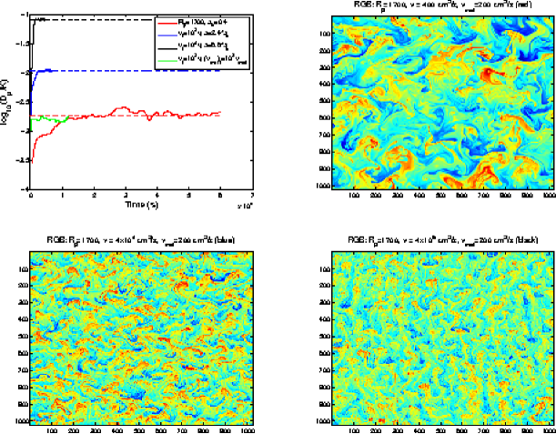
Figure 4: Snapshots and results of our 2D numerical simulations of thermohaline convection for the RGB case with the same density ratio $R_{\rho}=1700$ but for different values of viscosity and mixing rate. Upper-right panel: the standard RGB case (see Table 1). Lower-left and lower-right panels: the viscosity has been increased by the factors of $10^{2}$ and $10^{4}$ (assuming it is now of turbulent origin). Upper-left panel: the diffusion coefficients and effective finger aspect ratios corresponding to the cases presented in the other three panels. The green curve has the same parameter set as the blue curve except that its corresponding mixing rate (molecular diffusivity $\nu_{\rm mol}$) has also been increased by the factor of $10^{2}$.

The red curve from Fig. 3 is also plotted in the upper-left panel of Fig. 4, while the upper-right panel shows a snapshot of its corresponding salinity ($\mu$ in this case) field at equilibrium. A comparison of the latter panel with the upper panel of Fig. 2 leads us to the conclusion that, unlike the oceanic case, there are no visible vertically elongated structures (fingers) in the RGB case. This is the reason why we get $a<1$ in the second case. The $\mu$-field patterns in the upper-right panel of Fig. 4 instead resemble disorganized turbulent-like convection. A possible explanation of the difference in the salinity-field structures between the oceanic and RGB case can be given on a basis of results of the analysis of the equilibration of the salt-finger instability reported by Radko (2010). First of all, it should be noted that the difference between the two cases is evidently caused by their corresponding different values of the three dimensionless parameters in equations (18 – 20): $R_{\rho}$, $Pr$, and $\tau$ (the last three rows in Table 1). Radko (2010) replaced the original non-linear equations by their weakly non-linear analogs using asymptotic expansions in which $\varepsilon=1/R_{\rho}-\tau\ll 1$ and then he solved them numerically for a wide range of $Pr$ employing a computer code similar to that used by us. As a result, he has isolated two dominating mechanisms of salt-fingering equilibration. These are the triad interactions between various growing modes (e.g., Vallis 2006) and the adverse action of vertical shear, spontaneously developing as a result of secondary salt-finger instability. Radko (2010) has come to the conclusion that, although both processes are essential, it is the shear instability that becomes critical at $Pr\ll 1$. Under these circumstances, the growth of fingering salinity and heat fluxes is limited by the energy dissipation sufficient to balance the buoyancy forcing generated by the double-diffusive (primary) instability (Shen 1995). The fluxes generally decrease with the Prandtl number, although their dependence on $Pr$ is non-monotonic.

To verify these predictions for the RGB case, we have repeated our computations with the viscosity ($Pr\propto\nu$) artificially increased by factors of $10^{2}$ and $10^{4}$. The effective $\mu$-diffusivities for these test cases, as well as their approximations by the linear diffusion coefficient (15), are plotted with blue and black solid and dashed curves in the upper-left panel of Fig. 4. We see that the increase of $Pr$ indeed results in an increase of $D_{\mu}$, the latter being proportional to the $\mu$-flux. The linear approximation of $D_{\mu}$ for $\nu_{\rm t}=10^{4}\,\nu=4\times 10^{6}$ cm² s^-1 yields the effective finger aspect ratio $a\approx 6.6\,a_{0}=2.6$, where $a_{0}=0.4$ for the standard RGB case. We use a subscript “t” in the expression for viscosity to emphasize the fact that this cannot be a microscopic viscosity anymore. Instead, it could be a turbulent viscosity like the one associated with rotation-driven instabilities. When $\nu=4\times 10^{6}$ cm² s^-1, the $\mu$-field patterns, like the value of $a$, appear to almost be identical to those obtained for the oceanic case (compare the lower-right panel of Fig. 4 with upper panel of Fig. 2). The case of $\nu_{\rm t}=10^{2}\,\nu=4\times 10^{4}$ cm² s^-1 corresponds to a transition from the $\mu$-field structure at $\nu=4\times 10^{6}$ cm² s^-1 that looks more or less organized in the vertical direction to the structure resembling a turbulent-like convection at $\nu=400$ cm² s^-1. The most interesting pattern seen in the lower-left panel of Fig. 4 is something like a vertically varying sinusoidal shear. This is most likely to be a manifestation of the mean field effects (a secondary instability) that become critical at low $Pr$, according to Radko (2010). It is also interesting to compare our snapshot panels corresponding to the decreasing $\nu$ with the sequence of $T$-field snapshots presented in Fig. 2 by Shen (1995). They look very similar. However, the important difference is that Shen shows a time sequence along which the secondary instability, the one that leads to the equilibrium salt-fingering convection, is developing, whereas our sequence shows the equilibrium states already achieved for different values of $Pr$, at the highest of which the secondary instability appears to be strongly suppressed.

Our results in the upper-left panel of Fig. 4, in particular, the one represented by the black curve, could be used to support the hypothesis that the ³He-driven thermohaline convection is the main RGB extra-mixing mechanism, provided that a sufficiently strong turbulent viscosity, say of rotational origin (e.g., Palacios et al. 2006), would be present in the radiative zones of RGB stars. However, such a speculation has to admit (and explain how it is possible) that the turbulence enhances only the viscosity but not the $\mu$-diffusivity. Indeed, when we increase both $\nu$ and $\nu_{\rm mol}$ by the same factor, the effective thermohaline $\mu$-diffusivity returns close to its standard value (the green curve in the upper-left panel of Fig. 4). This is not surprising because an increase of $\nu_{\rm mol}$ ($k_{S}$ in the oceanic case) reduces the buoyancy force by making it faster for the difference in the chemical composition between rising and sinking blobs to be smoothed out horizontally (see the second term in the parentheses in eq. 15). Furthermore, if we accept the hypothesis that turbulence in stellar radiative zones should be highly anisotropic, with its associated horizontal viscosity components strongly dominating over that in the vertical direction (Zahn 1992), then the above speculation becomes even less likely, again provided that the chemical composition transport is accelerated by the turbulence proportionally to that of momentum.

4 Post-Processing 1D Simulations of the RGB Thermohaline Mixing

The results of our 2D numerical simulations of thermohaline convection in the vicinity of the HBS in the bump luminosity RGB model predict the effective salt-finger aspect ratio $a=0.4$ – $0.5$ that is an order of magnitude smaller than the one advocated by Ulrich (1972), the latter being needed to reproduce the Gratton et al. (2000) observational data, according to Charbonnel & Zahn (2007). The small value of $a$ in the RGB case compared to its much higher value in the oceanic case is due to the more favourable conditions for the development of secondary instabilities, that strongly limit the growth of salt fingers, at low Prandtl numbers.

However, our simulations are far from being perfect. Indeed, first of all, they are two-dimensional, in which case the oceanic salt-fingering fluxes were found to be underestimated by a factor of two to three compared to 3D numerical simulations (Radko & Stern 1999). For low Prandtl numbers corresponding to the RGB case, differences between the 2D and 3D solutions may be even more substantial (Radko 2010). Second, our simulations are restricted to a small space domain surrounding the point of minimum $R_{\rho}$. Third, they do not take into account either nuclear reactions or a modification of $R_{\rho}$ by thermohaline mixing, both of which may influence the growth of salt fingers. Finally, there still remains the possibility that the secondary instability associated with the mean field effects (vertical shear) can be suppressed in the RGB case, for example, by rotation-induced turbulence, such that the turbulent viscosity considerably exceeds the rate of turbulent mixing for some reason, which will result in a higher $a$. Therefore, we have decided to supplement our 2D numerical simulations of the RGB thermohaline convection with 1D computations of the evolutionary changes of the surface chemical composition of RGB stars above the bump luminosity in which we model the ³He-driven thermohaline convection using the linear-theory diffusion coefficient (15) as in the work of, e.g. Charbonnel & Zahn (2007) and Stancliffe et al. (2009). However, given that the diffusion coefficient (15) is proportional to an extremely small quantity $|\nabla_{\mu}|\lesssim 10^{-4}$, which is affected by the mixing itself, we decided that it would be very sensible to re-mesh the computational grid of full stellar evolution computations, and to perform our 1D simulations on a fixed mesh in a post-processing way. Our goal is to see if we can adjust a value of $a$ with which the diffusion coefficient (15) will really be able to reproduce the ¹²C/¹³C, C, and N data of Gratton et al. (2000). We want to do this also because there were some discrepancies between the results reported by Charbonnel & Zahn (2007) and Stancliffe et al. (2009), on the one side, and those obtained and anticipated by Denissenkov & Pinsonneault (2008b), on the other.

4.1 Basic Equations and a Method of Their Solution

Denissenkov & Pinsonneault (2008a) have noticed that, in the absence of extra-mixing, the $\mu$-profile in the radiative zone of an RGB star above the bump luminosity does not change very much if the mean molecular weight is plotted as a function of radius. The electron-degenerate He core in the center of the RGB star can be considered as a low-mass white dwarf, whose radius is known to weakly depend on its mass ($R\propto M^{1/3}$). The He core mass increases with time as the star climbs the RGB, thanks to the transformation of H into He taking place in the HBS atop the He core. This needs some fresh H to constantly be conveyed to the HBS from the base of convective envelope through the radiative zone. Note that, whereas the mass of the radiative zone is very small ($\sim 0.01$ – $0.001\,M_{\odot}$), its radius extends from a value of the order of the Earth’s radius at the He core boundary to a value of the order of the Sun’s radius at the base of the convective envelope. A typical radial velocity of the mass inflow between the envelope and HBS, that feeds H to the HBS, is $\dot{r}\approx-(10^{-4}$ – $10^{-5})$ cm s^-1. Given these facts, it is natural to write and solve the nuclear kinetics equations for the radiative zone in the Eulerian coordinates

$$\frac{\partial y_{i}}{\partial t}+\dot{r}\,\frac{\partial y_{i}}{\partial r}=\left(\frac{\partial y_{i}}{\partial t}\right)_{\rm nucl}+\frac{\partial}{\partial r}\left(D_{\mu}\,\frac{\partial y_{i}}{\partial r}\right),$$ (21)

where $y_{i}$ is the mole-per-gram abundance of the $i^{\rm th}$ nuclide, $D_{\mu}$ is the thermohaline diffusion coefficient given by expression (15) with $C=2C_{\rm Kunze}=2\pi^{2}$, and the first term on the right-hand side describes local changes of $y_{i}$ produced by nuclear reactions.

Distributions of $\rho(r)$, $T(r)$, and other stellar structure parameters in the radiative zone necessary for calculations of $\dot{r}$, $D_{\mu}$, and the nuclear term in (21) are taken from a couple of our MESA models separated by a sufficiently large distance in $\log L/L_{\odot}$ on the RGB, the first model being located immediately after the bump luminosity, where the RGB extra-mixing is supposed to commence. The models are used to interpolate the structure parameters in both $r$ and $t$. The mass inflow rate can be estimated from the mass and energy conservation relations

$$\frac{dr}{dt}=-\frac{1}{4\pi r^{2}\rho}\,\frac{dM_{r}}{dt},\ \ \ \ \frac{dM_{r}}{dt}=\frac{L}{\varepsilon_{\rm CN}X_{\rm e}},$$ (22)

where $X_{\rm e}$ is the envelope hydrogen mass fraction, $\varepsilon_{\rm CN}\approx 6\times 10^{18}$ erg g^-1 is the energy released per one gram of hydrogen burnt in the CN-branch of nuclear reactions, and $L$ is the star’s luminosity that is assumed to be constant in the radiative zone above the HBS. A comparison of these relations with real $\dot{r}$-profiles from our RGB models has led to the following corrected relation

$$\dot{r}\approx-0.6\,\left(\frac{L_{\odot}}{4\pi R_{\odot}^{2}\varepsilon_{\rm CN}}\right)\,\frac{L/L_{\odot}}{(r/R_{\odot})^{2}\rho X_{\rm e}}$$ (23)

that will be used in our 1D simulations.

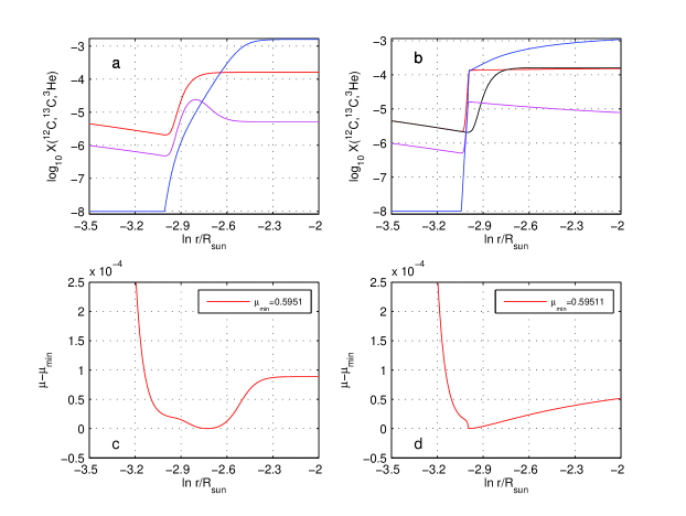
Figure 5: The ³He, ¹²C, and ¹³C abundance and $\mu$ profiles in the vicinity of the HBS in the bump luminosity model with $Z=0.001$ and $M=0.83\,M_{\odot}$ computed in the absence of extra-mixing (panels a and c). Panels b and d: the same profiles after they have been modified by RGB extra-mixing modeled by the diffusion coefficient (15) with $a=5$. The black curve in panel b is the same as the red curve from panel a.

Our test nucleosynthesis computations have shown that both the location and form of the $\mu$ depression are entirely determined by the reactions of ³He burning and those of the CN-branch of the CNO-cycle. Therefore, in our post-processing RGB extra-mixing simulations, we have included only the following reactions: ³He(³He,2p)⁴He, ³He($\alpha,\gamma)^{7}$Be(p,$\gamma)^{8}$B($\beta^{+}\nu_{\rm e}$) 2 ⁴He, ¹²C(p,$\gamma)^{13}$N($\beta^{+}\nu_{\rm e})^{13}$C, ¹³C(p,$\gamma)^{14}$N, ¹⁴N(p,$\gamma)^{15}$O($\beta^{+}\nu_{\rm e})^{15}$N, and ¹⁵N(p,$\alpha)^{12}$C. Their rates have been taken from the NACRE compilation by Angulo et al. (1999). The abundances of H, ³He, ⁴He, ¹²C, ¹³C, ¹⁴N, and ¹⁵N from the convective envelope of the MESA bump luminosity model are used as initial uniform conditions in the radiative zone. Simple boundary conditions, $(\partial y_{i}/\partial r)=0$, are applied at the bottom of the HBS, where $X=10^{-4}$, and at the star’s surface. Mixing in the convective envelope is modeled with the diffusion coefficient $D_{\rm conv}=10^{12}$ cm² s^-1, which keeps the envelope composition uniform. The system of equations (21) has been solved numerically by a finite element method using the COMSOL Multiphysics software package. Initially, we substitute $D_{\mu}=\nu_{\rm mol}$ into equations (21) and solve them using the stellar structure parameters only from the first model for a long enough time to determine stationary abundance and $\mu$ profiles in the background of the radiative zone mass-inflow (e.g., panels a and c in Fig. 5). After this, we switch on the ³He-driven thermohaline mixing and let it operate as our model evolves by adding the expression (15) to $D_{\mu}$ and interpolating the relevant stellar structure parameters in time and radius between our two RGB models. Note that the addition of (15) to the diffusion coefficient introduces an extra non-linearity in the PDEs (21) because of the dependence

$$D_{\mu}\propto\frac{\partial\ln\mu}{\partial\ln r}=-\mu\,\sum_{i}\,(1+Z_{i})\,y_{i}\,\frac{\partial\ln y_{i}}{\partial\ln r},$$ (24)

where $Z_{i}$ is the charge of the $i^{\rm th}$ nuclide. It is this non-linearity associated with extremely small values of the term $(\partial\ln\mu/\partial\ln r)$ plus the frequent re-meshing of the radiative zone needed because the HBS constantly advances in mass that make the implementation of the ³He-driven thermohaline mixing difficult in full stellar evolution computations. The researches who have done such calculations (e.g., Charbonnel & Zahn 2007, and Stancliffe et al. 2009) did not provide details of their implementations making it impossible to try to reproduce or assess their results. To eliminate a potential problem associated with the re-meshing, we solve the PDEs on a fixed mesh. To treat the non-linearity as precisely as possible, we use a large number of mesh points (approximately 1000) and set up very small tolerances in the time stepping algorithm of the COMSOL code.

4.2 Solutions for the Low-Metallicity RGB Models

A mean metallicity of upper RGB stars from the Gratton et al. (2000) sample with [C/Fe] abundances clearly demonstrating an evolutionary decline corresponds to the heavy-element mass fraction $Z\approx 0.0005$, with a dispersion comparable to the mean value. Their masses as estimated using the Hipparcos parallaxes are centered around $M\approx 0.85\,M_{\odot}$. Therefore, we will model the RGB extra-mixing in these stars using MESA RGB models that have $Z=0.001$ and $Z=0.0001$, and the masses $M=0.83\,M_{\odot}$ and $M=0.85\,M_{\odot}$, respectively. Panels a and c in Fig. 5 show the ³He, ¹²C, ¹³C, and $\mu$ profiles in the vicinity of the HBS in the bump luminosity model with $Z=0.001$ in the absence of extra-mixing. A rule of thumb for estimating a correct depth of the $\mu$ depression is the relation $\Delta\mu\approx\mu^{2}\Delta X(^{3}\mbox{He})/6$, where $\Delta X(^{3}\mbox{He})$ can be replaced with the envelope ³He mass fraction with no harm done. Applying this rule for $\log_{10}X_{\rm e}(^{3}\mbox{He})\approx-2.8$ and $\mu\approx\mu_{\rm min}=0.595$ (panels a and c), we obtain an estimate of $\Delta\mu\approx-9\times 10^{-5}$ that is close to the maximum depth of the $\mu$ depression in panel c.

The minimum of $\mu$ is reached at $\ln\,r_{\rm min}/R_{\odot}\approx-2.73$, or $r_{\rm min}/R_{\odot}\approx 0.065$, where $r_{\rm min}=r(\mu_{\rm min})$. This is very close to the values reported in our previous publications (e.g., Denissenkov & Pinsonneault 2008b). If we draw a vertical line through the point of $\mu_{\rm min}$ in panel c toward the panel a then we will come to our former conclusion that the ³He-driven thermohaline convection cannot explain the observed decline of [C/Fe] unless it penetrates below $\mu_{\rm min}$. It turns out that such overshooting is indeed possible, provided that the thermohaline mixing is much more efficient than the one predicted by our 2D numerical simulations. Panels b and d in Fig. 5 show the abundance and $\mu$ profiles that are obtained for a case of extra-mixing in which $D_{\mu}$ has been modeled by equation (15) with $a=5$. Note that this finger aspect ratio is nearly ten times as large as the effective one estimated from Fig. 3, the resulting diffusion coefficient being almost two orders of magnitude higher. Panels b and d correspond to a short time after the mixing has been switched on. We see that the mixing extends down to the radius $r_{\rm mix}\approx 0.05\,R_{\odot}$. Again, this is close to the mixing depth used by Denissenkov & Pinsonneault (2008a). Although the overshooting from $r_{\rm min}$ to $r_{\rm mix}$ has been produced numerically, it has some physical justification, and can therefore be real. When the mixing is switched on, it will first steepen the $\mu$-profile immediately to the right from $r_{\rm min}$ (panel c). Very soon, this will result in the formation of a discontinuity in the $\mu$-profile at $r_{\rm min}$, where material with a higher $\mu$ overlies material with a lower $\mu$. Such a stratification is also subject to the double-diffusive instability, like the one with uniform salinity and temperature gradients considered previously. Hence, the material from the right will start to mix with the material from the left, thus pushing the $\mu$-profile discontinuity to the left and, simultaneously, lowering it. This process will continue until the point $r_{\rm mix}$ is reached at which the local reduction of $\mu$ by ³He burning, with ³He being conveyed by mixing from the envelope, is balanced by the increase of $\mu$ caused by the transformation of H into He in the CN-cycle.

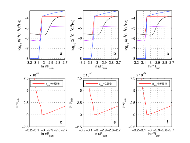
Figure 6: The first pair of the upper and lower panels (a and d) is the same as panels b and d in the previous figure, while the other two pairs correspond to finger aspect ratios $a=6$ and $a=7$, respectively.

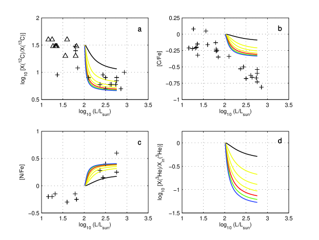
Figure 7: The evolutionary changes of the surface ¹²C/¹³C ratio (panel a) and the abundances of C (panel b) and N (panel c) in the field low-metallicity and low-mass RGB stars studied by Gratton et al. (2000) (crosses and triangles, the latter showing upper limits). Curves represent theoretical reproductions by our model of RGB extra-mixing with $Z=0.001$ and $M=0.83\,M_{\odot}$ in which mixing is described by the diffusion coefficient (15) with $a=1$ (black curves), $a=2$, 3, and 4 (yellow curves), $a=5$ (red curves), $a=6$ (green curves), and $a=7$ (blue curves). Panel d shows the unobserved decline of the envelope ³He abundances that is predicted theoretically.

Fig. 6 compares the abundance and $\mu$ profiles for $a=5$ (panels a and d), $a=6$ (panels b and e), and $a=7$ (panels c and f) in the same bump luminosity model. Black curves in the three upper panels show the ¹²C profile in the model without mixing (the red curve in Fig. 5a). One can see that the mixing with the higher finger aspect ratio penetrates deeper into the HBS and, at the same time, its diffusion coefficient is increased proportionally to $a^{2}$ (eq. 15). However, this does not turn out to strongly change the evolutionary variations of the surface composition produced by the mixing with the large values of $a$. They are plotted with red ($a=5$), green ($a=6$), and blue ($a=7$) curves in Fig. 7, where crosses and triangles represent the Gratton et al. (2000) data, the triangles showing upper limits to the ¹²C/¹³C ratio. For comparison, black curves in Fig. 7 correspond to the case of $a=1$. Note that even this small finger aspect ratio still leads to a nearly four times larger thermohaline diffusion coefficient than the one predicted by our 2D numerical simulations (the red curve in Fig. 3).

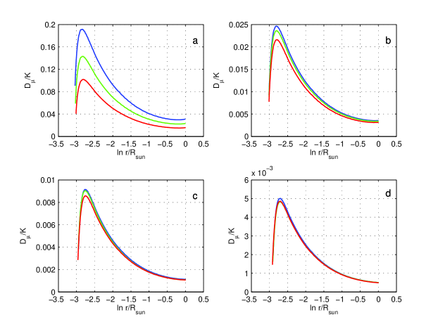
Figure 8: Convergence of the diffusion coefficient profiles for the models presented by the same colors in the previous figure. Panels a, b, c, and d show how the results vary with time. Each panel is separated, in turn, by a time interval that is approximately equal to 20% of the total time for which the models have been evolved.

Denissenkov & VandenBerg (2003) have demonstrated that an increase of the RGB extra-mixing rate by the factor of two should result in a strong enhancement of the evolutionary decline of the carbon abundance (see their Fig. 7). An increase of the mixing depth should also enhance the [C/Fe] depletion, though in a lesser proportion than that of the diffusion coefficient (their Fig. 8). In the present case, it turns out that, in spite of the fact that the increase of $a$ from 5 to 7 doubles the diffusion coefficient (15) and, at the same time, produces deeper mixing, this does not affect the [C/Fe] evolutionary decline (compare the red and blue curves in Fig. 7b) very much. This difference is explained by a convergence of the diffusion coefficients (15) calculated for different but sufficiently large values of $a$ to the same profile (Fig. 8), as ³He gets depleted in the envelope (Fig. 7d). The faster and deeper mixing destroys ³He quicker than the slower and shallower mixing and, because the diffusion coefficient (15) is indirectly proportional to the mass fraction of ³He left in the envelope (through the dependence $\Delta\mu\propto\Delta X(^{3}\mbox{He})$), the $D_{\mu}$-profile corresponding to the larger value of $a$ quickly converges to that calculated for the smaller $a$. In other words, it can be said that the efficient ³He-driven thermohaline mixing becomes self-quenching. On the contrary, the aforementioned results reported by Denissenkov & VandenBerg (2003) were obtained for constant mixing rates. In connection to this, it should be noted that Denissenkov & Pinsonneault (2008b) have reproduced the Gratton et al. (2000) data with the diffusion coefficient $D_{\rm mix}=0.02\,K$ also assuming that it does not change with time. Therefore, given that the coefficient (15) rapidly decreases with time as a result of the self-quenching (Fig. 8), its initial values have to be much larger than $0.02\,K$ (Fig. 8a). Hence, the green line in the upper panel of Fig. 3 with which we have compared our 2D numerical simulations of the thermohaline diffusion coefficient should be increased by approximately one order of magnitude.

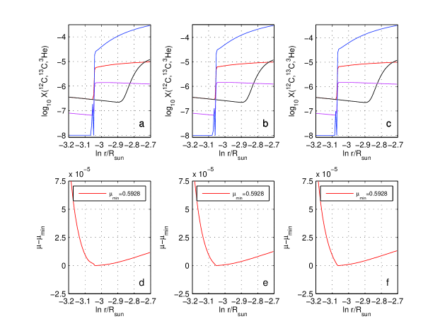
Figure 10: Same as in Fig. 6 but for the bump luminosity model with $Z=0.0001$ and $M=0.85\,M_{\odot}$.

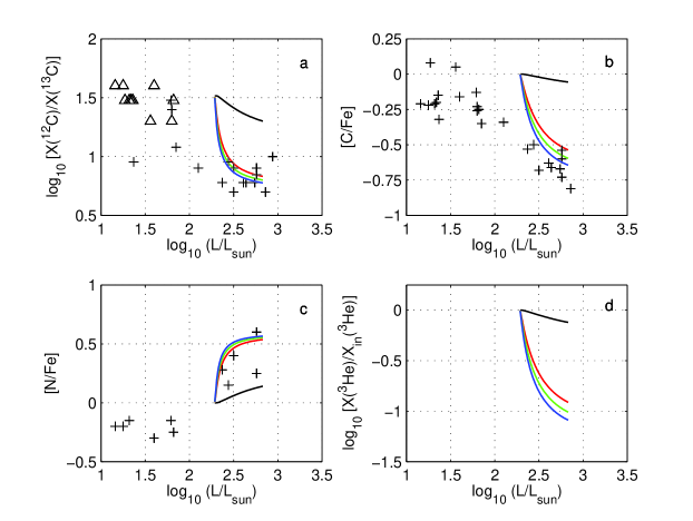
Figure 11: Same as in Fig. 7, except that the yellow curves are omitted, but for the RGB model with $Z=0.0001$ and $M=0.85\,M_{\odot}$.

The floor of the $\mu$ depression is found to be almost flat in the case of $Z=0.0001$ and $M=0.85\,M_{\odot}$ (Fig. 9c). As a result, for the same value of $a=5$, the mixing in this model penetrates deeper (with respect to the ¹²C profile in the unmixed model, shown with black curves in Figs. 5b and 9b) than in the model with the higher metallicity (compare panels b and d in the two figures). As in the previous case, the mixing depth increases with $a$ (Fig. 10). Given that the bump luminosity is higher for the lower metallicity model, the mixing in it starts with a larger initial $K$, hence with a higher $D_{\mu}\propto K$, because $K\propto L$ but, at the same time, the mixing has less time to accomplish its task. Evolutionary changes of the surface chemical composition produced by the mixing are shown in Fig. 11. We see that the low [C/Fe] ratios in the most luminous RGB stars from the Gratton et al. sample are almost reproduced with the diffusion coefficient (15), provided that the finger aspect ratio can reach a value of $a\gtrsim 7$. Note, however, that this result is obtained for $Z=0.0001$, whereas some of these stars have metallicities closer to $Z=0.001$, in which case the agreement between our model predictions and the observational [C/Fe] data is worse (Fig. 7b). Nevertheless, given the model uncertainties, the approximations used in our 1D simulations of the RGB thermohaline mixing, and the fact that the metallicities of upper RGB stars from the Gratton et al. sample are distributed between $Z\approx 0.001$ and a value of $Z$ close to 0.0001, we find the general agreement between the linear theory with the high finger aspect ratios and observations to be satisfactory. Besides, the model confirms the observational inference that the effect of the RGB extra-mixing increases towards lower metallicities. Thus, the results of our 1D simulations of ³He-driven thermohaline mixing in upper RGB stars go along with those reported by Charbonnel & Zahn (2007). In particular, even our adjusted finger aspect ratio $a=7$ results in a value of the total non-dimensional coefficient $C_{\rm t}=2\pi^{2}a^{2}=967$ that is very close to the value of $C_{\rm t}=1000$ used by them.

4.3 Solutions for the Solar-Metallicity RGB Model

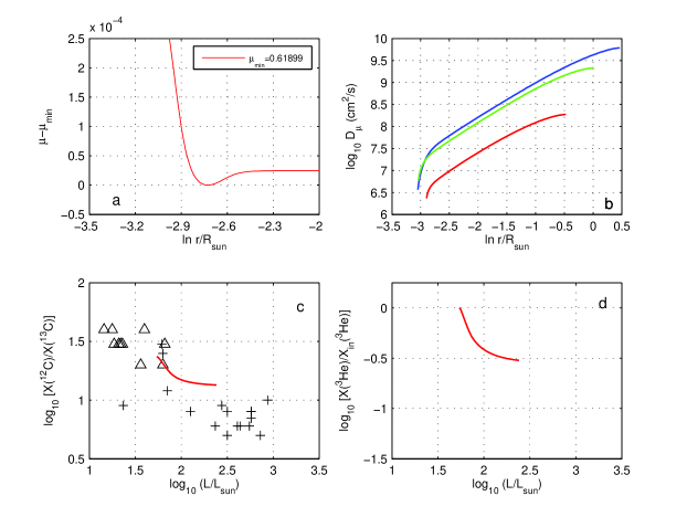
Figure 12: The $\mu$ and $D_{\mu}$ profiles and the evolutionary changes of the ¹²C/¹³C ratio and abundance of ³He computed for the RGB model with $Z=0.0188$ and $M=1.5\,M_{\odot}$ using the diffusion coefficient (15) with $a=7$ (red curves). The blue and green curves in panel b show the $D_{\mu}$ profiles from the bump luminosity models with $Z=0.0001$ and $Z=0.001$, respectively.

The $\mu$-profile in the vicinity of the HBS in our MESA bump luminosity model with $Z=0.0188$ and $M=1.5\,M_{\odot}$ is plotted in Fig. 12. It is shown in the absence of mixing. It has two important differences, as compared to the $\mu$-profiles in the low-metallicity models, by being shallower and narrower. The first property means that the ³He-driven thermohaline mixing in the solar-metallicity RGB star should be much slower than that in low-metallicity red giants for the same finger aspect ratio. A comparison of the coefficients $D_{\mu}$ for our three MESA models calculated using equation (15) with $a=7$ confirms this conclusion (Fig. 12). The second property means that the mixing in the solar-metallicity model cannot penetrate as deep into the HBS as it did in the low-$Z$ models. As a result, it cannot dredge up carbon depleted material and, therefore, does not affect the surface [C/Fe] abundance at all. The only visible abundance changes that it can cause are Li depletion, and a modest reduction of the carbon isotopic ratio (Fig. 12). It is interesting that the linear theory (eq. 15) with $a=7$ predicts that ³He-driven thermohaline mixing in the solar-metallicity RGB star should lead to ¹²C/${}^{13}\mbox{C}\approx 12$ – $14$, which is very close to the abundance ratios measured in upper RGB stars in the open cluster M 67 (Gilroy & Brown 1991), which has nearly the solar metallicity and an MS turn-off mass of about $1.3\,M_{\odot}$ (e.g., VandenBerg & Stetson 2004). This result shows that the ³He-driven thermohaline mixing modeled by the diffusion coefficient (15) with the finger aspect ratio $a\gtrsim 7$ can indeed reproduce properly the evolutionary abundance changes observed in upper RGB stars of all metallicities, a conclusion similar to that obtained by Charbonnel & Zahn (2007). Having said that, we emphasize that our 2D numerical simulations predict $a<1$; in which case, the model of the RGB thermohaline mixing fails to interpret the observations (the black curves in Figs. 6 and 10).

Li-rich giants may pose another problem for the explanation of the RGB extra-mixing by the ³He-driven thermohaline convection. These stars have masses and metallicities close to those of our solar-metallicity MESA model, and most of them are located near the bump luminosity (Charbonnel & Balachandran 2000). Denissenkov & Herwig (2004) have shown that the anomalously large abundances of Li in these stars can be explained by the “⁷Be-transport” mechanism (Cameron & Fowler 1971) only if their radiative zones experience extra-mixing with a significantly enhanced diffusion coefficient (up to $10^{11}$ cm² s^-1). The blue curve in Fig. 12 corresponds to $a=7$ but it only reaches values of the order of $D_{\mu}\sim 10^{8}$ cm² s^-1. To obtain the values necessary for efficient Li production, we have to assume $a\approx 200$, which does not seem realistic. Hence, we would rather attribute the enhanced extra-mixing in Li-rich giants to some alternative mixing process that replaces thermohaline convection in these stars. However, we think this would be inconsistent because it is difficult to understand why this alternative mixing process cannot be the universal one that operates both in the Li-rich giants, which represent a few percent of all upper RGB stars, and in all other upper RGB stars in which its efficiency is reduced to $D_{\rm mix}\sim 10^{8}$ – $10^{9}$ cm² s^-1 for some reason. Drake et al. (2002) have reported that, in their sample of single K giants “among rapid ($v\sin i\gtrsim 8$ km s^-1) rotators, a very large proportion ($\sim$50%) are Li-rich giants” and that “this proportion is in contrast with a very low proportion ($\sim$2%) of Li-rich stars among the much more common slowly rotating K-giants”. This correlation of the RGB extra-mixing enhancement (needed for the Li enrichment) with the rapid rotation has been used by Denissenkov & Herwig (2004) to speculate that the RGB extra-mixing is actually driven by rotation and that the Li-rich giants had been spun up as a result of their engulfing of massive planets. Note that, although Palacios et al. (2006) have claimed that the RGB extra-mixing cannot be associated with a pure rotational mechanism, there is still a possibility that an interaction of rotation and large-scale magnetic fields can drive the mixing (Busso et al. 2007; Denissenkov, Pinsonneault, & MacGregor 2009). The only scenario that could explain this correlation in the model with thermohaline mixing would be to assume that the Li-rich giants swallowed low-mass MS companions that are enriched in ³He. This could explain the rapid rotation (a deposit of orbital angular momentum) and probably the speed-up of extra-mixing by the increased amount of ³He that was supplied externally. However, from our point of view, this scenario appears to be too complicated, and therefore highly improbable.

Finally, a comparison of panels d in Figs. 6, 10, and 12 leads to the conclusion that, whereas ³He gets strongly depleted in the low-metallicity RGB stars, its envelope abundance is reduced by a factor of only a few in the solar-metallicity model. On the one hand, this can be used as an argument against ³He-driven thermohaline convection as the mechanism of RGB extra-mixing if the presence of similar extra-mixing process in low-metallicity AGB stars with masses $M\lesssim 1\,M_{\odot}$ surmised by Masseron et al. (2006) and Lebzelter et al. (2008) will by confirmed by other observations. On the other hand, if the observational abundance anomalies, in particular those in meteorites (e.g., Nollett, Busso, & Wasserburg 2003), suggest the operation of an RGB-like extra-mixing only in the population I AGB stars with masses $M\gtrsim 1\,M_{\odot}$ (Busso et al. 2010), then a more detailed analysis of the consequences of modest ³He depletion in the solar-metallicity RGB model for the following AGB thermohaline mixing driven by ³He burning is still needed, especially given the arguments against this hypothesis presented by Karakas, Campbell, & Stancliffe (2010). We will provide such the analysis in our forthcoming paper.

5 Discussion and Conclusions

In this work, we have come to the following two conclusions that happen to contradict one another. On the one hand, the linear stability analysis of the Boussinesq equations (1 – 3) with parameters set up to describe the growth of salt fingers driven by ³He burning in the vicinity of the HBS in a low-mass RGB star above the bump luminosity leads to the thermohaline diffusion coefficient (15). It models surprisingly well the observed evolutionary changes of the surface chemical composition in upper RGB stars of different metallicities, provided that we employ the empirically constrained finger aspect ratio $a_{\rm obs}\gtrsim 7$. In other words, we arrive at a solution very similar to that proposed by Charbonnel & Zahn (2007), namely that the effects of the RGB extra-mixing can be reproduced in stellar evolutionary computations if the simple diffusion coefficient

$$D_{\mu}=2\pi^{2}a_{\rm obs}^{2}\,\frac{\nabla_{\mu}}{\nabla_{\rm rad}-\nabla_{\rm ad}}\,K,$$ (25)

where $a_{\rm obs}\gtrsim 7$, is used. This large value of $a$ is close to the one advocated by Ulrich (1972). On the other hand, our 2D numerical simulations of thermohaline convection for the same RGB parameter set (Table 1) have shown that the effective finger aspect ratio in expression (15) does not exceed a value of $a_{\rm eff}\approx 0.5$. Interestingly, this small value of $a$ coincides with the one estimated by Kippenhahn et al. (1980). Because of the dependence of $D_{\mu}$ on the square of $a$, the difference between the two diffusion coefficients calculated with $a=a_{\rm obs}$ and $a=a_{\rm eff}$ exceeds two orders of magnitude. It is highly unlikely that our 2D numerical simulations have underestimated $D_{\mu}$ by this much. Therefore, we are inclined to conclude that RGB extra-mixing has nothing to do with salt-fingering transport and that alternative mixing mechanisms are worth investigating.

There is a clear physical explanation as to why salt-fingering leads to the turbulent convection in the RGB case, while it produces vertically elongated quasi-laminar structures (salt fingers) in the oceanic case (e.g., Shen 1995; Radko 2010). The main reason for the different outcome is the large difference in the Prandtl number (Table 1). The low Prandtl number (lower viscosity compared to heat diffusivity) in the RGB case favours the development of secondary instabilities, predominantly the one associated with the mean field effects of vertical shear, which do not allow the salt fingers to grow longer than their diameters in the vertical direction. We have demonstrated that the artificial increase of viscosity does stabilize the growth of salt fingers, as expected. In real RGB stars, such an increase could be associated with turbulence generated by rotation-driven instabilities, in which case the turbulent viscosity $\nu_{\rm t}$ may exceed the microscopic (molecular plus radiative) viscosity $\nu$ by several orders of magnitude (e.g., Zahn 1992; Palacios et al. 2006). However, it is difficult to imagine how the turbulence can affect only the viscosity without enhancing chemical mixing at the same time. Hence, we also have to replace $\nu_{\rm mol}$ by $\nu_{\rm t}$ in the expression in the parenthesis in the thermohaline diffusion coefficient (15) that has been omitted in (25) for the sake of simplicity, because it can be neglected in the absence of turbulence. This replacement counterbalances the stabilizing effect of higher turbulent viscosity because turbulent mixing, especially when it prevails in the horizontal direction (Zahn 1992), facilitates the smoothing out of the mean molecular weight contrast between the rising and sinking fingers, thus weakening the buoyancy force. In connection with this, it is important to note that the hypothesis that RGB extra-mixing is only partially executed by the ³He-driven thermohaline convection and that some other mixing mechanisms of rotational or magnetic origin are assisting it (e.g., Cantiello & Langer 2010), does not seem to be plausible. Indeed, we know from the comparison of simple mixing models with the observations that extra-mixing in the majority of low-mass upper RGB stars needs a diffusion coefficient of the order of $D_{\rm mix}\approx 0.02\,K$ (Denissenkov & Pinsonneault 2008b). If this mixing is associated with a mechanism different from that of the salt-fingering convection then we have to use the ratio $D_{\rm mix}/K\approx 0.02$ instead of $\nu_{\rm mol}/K$ in the parenthesis in the expression (15). Given that $R_{\rho}=(\nabla_{\rm rad}-\nabla_{\rm ad})/\nabla_{\mu}\gtrsim 1000$ in the radiative zones of RGB stars, the expression in the parenthesis becomes negative, which means that the density stratification is now stable against the double-diffusive instability. Consequently, there are only two possibilities: RGB extra-mixing is either entirely executed by the ³He-driven thermohaline convection or it is the result of an entirely different mechanism. To answer this question with certainty, our next step is to carry out 3D numerical simulations of thermohaline convection for the RGB case.

Table 1: Correspondence Between Salt-Fingering Parameters

	Oceanic Case		RGB Case
Parameter	Notation	Value (cgs)	Notation	Value (cgs)
Viscosity	$\nu$	$10^{-2}$	$\nu$	$4\times 10^{2}$
Thermal Diffusivity	$k_{T}$	$1.4\times 10^{-3}$	$K$	$10^{8}$
Haline Diffusivity	$k_{S}$	$1.1\times 10^{-5}$	$\nu_{\rm mol}$	$2\times 10^{2}$
Gravitational Acceleration	$g$	$9.8\times 10^{2}$	$g$	$10^{6}$
Thermal Expansion	$\alpha$	$2\times 10^{-4}$	$\alpha\approx T^{-1}$	$10^{-7}$
Haline Contraction	$\beta$	$7.5\times 10^{-4}\ {{}^{0}/_{00}}^{-1}$	$\beta\approx\mu^{-1}$	$1.7$
Temperature Gradient	$\frac{\partial T_{0}}{\partial z}$	$3\times 10^{-3}$	$\frac{\partial T_{0}}{\partial z}-\left(\frac{\partial T}{\partial z}\right)_{\rm ad}$	$2\times 10^{-3}$
Density Ratio	$R_{\rho}$	$1.6$	$R_{\rho}=(\nabla-\nabla_{\rm ad})/\nabla_{\mu}$	$1.7\times 10^{3}$
Prandtl Number ($\nu/k_{T}$)	$Pr$	$7$	$Pr$	$4\times 10^{-6}$
Inverse Lewis Number ($k_{S}/k_{T}$)	$\tau$	$8\times 10^{-3}$	$\tau$	$2\times 10^{-6}$

References

- Angulo et al. (1999) Angulo, C., Arnold, M., Rayet, M., et al. 1999, NuPhA, 656, 3
- Busso et al. (2007) Busso, M., Wasserburg, G. J., Nollett, K. M., & Calandra, A. 2007, ApJ, 671, 802 (BWNC)
- Busso et al. (2010) Busso, M., Palmerini, S., Maiorca, E., Cristallo, S., Straniero, O., Abia, C., Gallino, R., & La Cognata, M. 2010, ApJ, 717, L47
- Cameron & Fowler (1971) Cameron, A. G. W., & Fowler, W. A. 1971, ApJ, 164, 111
- Cantiello & Langer (2010) Cantiello, M., & Langer, N. 2010, arXiv:1006.1354v1 [astro-ph.SR]
- Canuto et al. (1988) Canuto, C., Hussaini, M. Y., Quarteroni, A., & Zang, T. A. 1988, Spectral Methods in Fluid Mechanics, Springer, New York
- Charbonnel (1994) Charbonnel, C. 1994, A&A, 282, 811
- Charbonnel (1995) Charbonnel, C. 1995, ApJ, 453, L41
- Charbonnel & Balachandran (2000) Charbonnel, C., & Balachandran, S. C. 2000, A&A, 359, 563
- Charbonnel & Zahn (2007) Charbonnel, C., & Zahn, J.-P. 2007, A&A, 467, L15
- Denissenkov & Tout (2000) Denissenkov, P. A., & Tout, C. A. 2000, MNRAS, 316, 395