Species assembly in model ecosystems, I: Analysis of the population model and the invasion dynamics.

Abstract

Recently we have introduced a simplified model of ecosystem assembly (Capitán et al., 2009) for which we are able to map out all assembly pathways generated by external invasions in an exact manner. In this paper we provide a deeper analysis of the model, obtaining analytical results and introducing some approximations which allow us to reconstruct the results of our previous work. In particular, we show that the population dynamics equations of a very general class of trophic-level structured food-web have an unique interior equilibrium point which is globally stable. We show analytically that communities found as end states of the assembly process are pyramidal and we find that the equilibrium abundance of any species at any trophic level is approximately inversely proportional to the number of species in that level. We also find that the per capita growth rate of a top predator invading a resident community is key to understand the appearance of complex end states reported in our previous work. The sign of these rates allows us to separate regions in the space of parameters where the end state is either a single community or a complex set containing more than one community. We have also built up analytical approximations to the time evolution of species abundances that allow us to determine, with high accuracy, the sequence of extinctions that an invasion may cause. Finally we apply this analysis to obtain the communities in the end states. To test the accuracy of the transition probability matrix generated by this analytical procedure for the end states, we have compared averages over those sets with those obtained from the graph derived by numerical integration of the Lotka-Volterra equations. The agreement is excellent.

1 Introduction

A piece of common wisdom in ecology is that biodiversity enhances the stability of ecosystems. This has traditionally been a well established observational fact since the works of Odum (1953), MacArthur (1955) and Elton (1958) who showed that simple ecosystems (e.g. man-cultivated lands) undergo very large fluctuations in population and are vulnerable to invasion, an effect that gets reduced upon increasing the number of predators and preys in the system. But early in the 70s May showed that randomly generated dynamical models for the populations of a community exhibit the opposite feature: the larger the species abundance the smaller its linear stability (May, 1972, 1973). Thanks to this controversy we have gained very much insight into the nature of ecosystems (McCann, 2000). Apart from the introduction of more refined concepts of ecosystem stability (Pimm, 1982), one of the main conclusions arising from the comparison of empirical data with May’s predictions on the bounds for community stability (Dunne, 2006) is that real ecosystem are within the tiny set of stable ones, no matter how large they are; in other words, ecosystems are far from being just random gatherings of species.

Natural communities carry out a selection mechanism that induces colonizers adaptation. There has been a lot of theoretical work in the past devoted to study the assembly of communities through successional invasions (Post and Pimm, 1983; Drake, 1990; Case, 1990; Law and Morton, 1993, 1996; Morton and Law, 1997). Overall, these papers have provided a theoretical framework to understand how communities are built up (Law, 1999). The basic process in which these models are based is the sequential arrival of rare species (invaders) that colonize the ecosystem and that may be established, possibly causing a global reconfiguration of the community in the long term by means of several species extinctions. Obviously, these models are but idealizations of the complex processes taking place in real community assembly, but simple mechanisms acting in these models could be expected to be the ones responsible for the formation of real ecosystems (Law, 1999). This approach of devising theoretical paradigms for real situations has been successfully applied over and over in the field of statistical mechanics —where, for instance, using such an idealization as the Ising model provides the clues to understanding ferromagnetism in real materials (Huang, 1987).

Previous assembly models tend all to rely on the Lotka-Volterra dynamics [but see the recent work of Lewis and Law (2007)], although differ in the criterion to accept an invasion. While Post and Pimm (1983) assumed that new species were created ad hoc, according to certain stochastic rules, subsequent approaches (Drake, 1990; Law and Morton, 1996) introduced the concept of “species pool”. A regional species pool is a set of possible invaders whose trophic interactions have been determined in advance (Law and Morton, 1996). Despite these differences, all previous papers arrive at the conclusion that the species richness of each resident community increases along successional time, although the average resistance of a community to be colonized increases in time. Therefore community assembly increases biodiversity as well as stability, understood as resistance to invasions.

Nevertheless, one must bear in mind that not all assembly pathways have been explored in these models. The conclusions reached so far rely on averages of quantities under study over a finite set of realizations of the underlying stochastic process, that is ultimately based on a finite pool of possible invaders. This has raised several question that remained without a definitive answer. For example, there was no clear-cut answer regarding the dependence of the results on the history of invasions. Morton and Law (1997) found a final end state resistant to invasions by the remaining species in the pool at the end of the process, and this end state could be either a single ecosystem or a set involving more than one community connected by invasions with one another. Despite this conclusion, the dependence of the end state on the assembly history is a matter of discussion (Fukami and Morin, 2003). Moreover, we should not forget that the number of species in the pools employed is always relatively small, so the question remains as to whether larger pools lead to qualitatively different results. In this respect, it has been pointed out (Case, 1991; Levine and D’Antonio, 1999) that the exhaustion of good invaders in the early assembly might be just an artifact of the finiteness of the pool.

Trying to overcome the shortcomings of previous models, in our previous work Capitán et al. (2009) we proposed a minimalistic model of ecosystem assembly with which we were able to analyze all assembly pathways, thus characterizing the full assembly process. In spite of its simplicity, we recovered the same conclusions found previously. Our model is also based on a pool of species and a niche variable (the trophic level) that determines their interactions. In contrast, however, our pool is infinite. In spite of that, within the assumptions of the model, we found a finite number of (viable) communities linked by colonization. This allowed us to define an assembly graph for our model —similar to that of Warren et al. (2003), who studied the assembly process experimentally for a small pool of 6 protist species. By assigning transition probabilities to the links of this graph the assembly process was mapped to a Markov chain (Karlin and Taylor, 1975), which is tantamount to saying that we defined a statistical mechanics on the set of viable communities (microstates). In other words, our model gives the probability distribution of all these microstates at any time. This allowed us to characterize both transient and equilibrium states, as well as to compute the time evolution of any observable along the assembly in an exact manner. But more importantly, as our model provides a complete and exact (albeit numeric) description of the assembly process, we can positively state that, under the assumptions of our model, in the long-term assembly dynamics a unique enstate is reached, and this state is formed by just one uninvadable community or a closed set of communities connected between them. These sets contain the communities that survive in the long term, and the ecosystem can be regarded as a fluctuating community that can vary each level occupancy trough successional invasions.

In this paper we will give some analytical results for the underlying population dynamics of our assembly model, and we will see how these results can be combined together to arrive at the same conclusions we obtained numerically in our previous work. Relying on these analytic results, we will be able to describe the observables that characterize the end states with high accuracy. In particular, we will reproduce the variation of the number of communities in each end state with the abundance of abiotic resources, as well as the average values of quantities like the species richness. We will leave the computational and numerical results that can be obtained with this model for the second paper of this suite (Capitán et al., 2010), which will be focused in the successional variation of biologically relevant quantities along the assembly, and the analysis of the main properties of transient states.

This paper is organized as follows. Section 2 is devoted to the analysis of a rather general model of trophic-level structured food-webs, and the discussion of its dynamic stability. In Section 3 we will restrict ourselves to a particular case of community by making a species symmetry assumption, that renders our model closer to neutral models and allows a more detailed analytical study. In Section 4 we will deduce some analytical properties of the equilibrium point, such as estimations of the maximum number of species allowed in a community for a given set of parameters, or the maximum number of trophic levels that the amount of resource allows. Section 5 is dedicated to discussing some criteria for an invader to establish in a community, and to give some global analytical approximations to the time evolution of a system invaded by a top predator. Finally, in Section 6 we will apply our analysis to recover the results obtained in Capitán et al. (2009) by means of a numerical integration of the population dynamics equations.

The two papers of this suite are self-contained and can be read separately, although they are cross-referenced. Readers interested in the underlying population dynamics of our model will find a detailed discussion in this paper. Those readers more interested in the ecological consequences and results that the model provides can skip the technical Sections 4 and 5. For a full account of the results that we have obtained, we refer them to the companion paper.

2 Trophic-level structured food-webs

How species are arranged in a network to conform a food-web is a question difficult to answer. The specific topology of the network where feeding interactions take place is very complex and several complicated models have been proposed for both the structure and the dynamics of food-webs (Dunne, 2006). In contrast, our aim in Capitán et al. (2009) was to construct a minimalistic model, so we considered the traditional picture of trophic pyramids of interacting species in different, well defined trophic levels. Although trophic levels can be roughly described in real webs (Martinez et al., 2006), we will assume that feeding interactions take place strictly between species belonging to contiguous, well defined trophic levels. This is a standard (and accurate) assumption, as the models of tri-trophic food chains show (Bascompte and Melián, 2005). This notwithstanding, it is acknowledged that omnivory, i.e. predation from several levels, exists although is still an open question how common it is. For example, work on food-web motifs has found that omnivory is sometimes under-represented and sometimes over-represented in real networks (Bascompte and Melián, 2005). However, the impact of including omnivory in the model could lead to non trivial results. Since the trophic level is normally related to species size, feeding from lower levels will provide less energy to predators, so proper allometric relations should be included in the model to fix the interaction strengths. For the sake of simplicity, we will not divert ourselves from the standard assumption of disregarding omnivory.

Therefore, any species at level $\ell$ will feed only on species at level $\ell-1$ and will be predated only by species at level $\ell+1$. Let $s_{\ell}$ be the number of species in the $\ell$-th level. Thus for an ecological community with $L$ trophic levels the total number of species is $S=\sum_{\ell=1}^{L}s_{\ell}$. In order to determine which species are predated at each level, we define the set of interaction matrices $\Gamma^{\ell}$, with dimensions $s_{\ell}\times s_{\ell-1}$, such that the element $\Gamma_{ij}^{\ell}=1$ when species $j$ in level $\ell-1$ is a prey of species $i$ in level $\ell$, and is zero otherwise. Any particular choice of this set of matrices determines the food-web in our model.

According to our aim of developing a simplified model, we propose a simple population dynamics with the purpose of capturing on average the main behavior of species abundances. It is inspired in a model used before to study coexistence in competing communities (Lässig et al., 2001; Bastolla et al., 2005a, b). Population dynamics is modelled by Lotka-Volterra equations, including both predator-prey interactions as well as intra- and interspecific competition. Thus, in order to keep the model minimalistic we have chosen not to include other interaction types such as mutualism.

Let $n^{\ell}$ be a column vector with the population densities of all the species at trophic level $\ell$. Following Bastolla et al. (2005a) we propose the mean-field dynamics

$$\frac{\dot{n}_{i}^{\ell}}{n_{i}^{\ell}}=\left(-\alpha+\gamma_{+}^{\ell}\Gamma^{(\ell)}n^{\ell-1}-B^{\ell}n^{\ell}-\gamma_{-}^{\ell}(\Gamma^{\ell+1})^{\rm T}n^{\ell+1}\right)_{i}.$$ (1)

We assume that the strength of the feeding interactions between contiguous levels is fixed and determined by the constants $\gamma_{+}^{\ell}$, which control the amount of energy available to reproduction for each predation event for species at level $\ell$, and $\gamma_{-}^{\ell}$ $(>\gamma_{+}^{\ell})$, which take into account the mean damage caused by predation over level $\ell$. The ratio $\gamma_{+}^{\ell}/\gamma_{-}^{\ell}$ measures the efficiency of conversion of prey biomass into predator biomass.

Interspecific competition in a trophic level is measured by the off-diagonal elements of the $s_{\ell}\times s_{\ell}$ matrix $B^{\ell}$, while intraspecific competition (diagonal elements) is normalized to unity (this just amounts to fixing a time scale for the dynamics). A natural way to represent this matrix is

$$B^{\ell}=(1-\rho^{\ell})\mathbb{I}+\rho^{\ell}K^{\ell},$$ (2)

where $\rho^{\ell}\leq 1$ measures the relative magnitude between intra– and interspecific competition, and $\mathbb{I}$ is the identity matrix. Diagonal elements of $K^{\ell}$ are equal to 1 due to the normalization of the intraspecific competition. We will assume (the reasons will become clearer later) that the competition matrix is symmetric and positive definite.

Interspecific competition due to sharing common preys is implicitly represented in the predation terms. There is however a direct competition due to other effects, such as territorial competition, mutual aggressions, etc. We will assume [as in Bastolla et al. (2005b)] that species sharing more preys are closely related ecologically [this fact might have support from a evolutionary viewpoint as shown in Rezende et al. (2007)], so their requirements are similar and we can assume that elements of $K^{\ell}$ are proportional to the ecological overlapping between species (Lässig et al., 2001; Bastolla et al., 2005b). Let $\pi_{ij}^{\ell}$ represent the number of common preys for species $i$ and $j$ belonging to level $\ell$. The species overlapping due to common preys is $K_{ij}^{\ell}=\pi_{ij}^{\ell}/\sqrt{\pi_{i}^{\ell}\pi_{j}^{\ell}}$, with $\pi_{i}^{\ell}$ the total number of preys of species $i$. Under our matrix notation, $\pi_{ij}^{\ell}=(\Gamma^{\ell}{\Gamma^{\ell}}^{\rm T})_{ij}$ and $\pi_{i}^{\ell}=(\Gamma^{\ell}{\Gamma^{\ell}}^{\rm T})_{ii}$, so that

$$B^{\ell}=(1-\rho^{\ell})\mathbb{I}+\rho^{\ell}D^{\ell}\Gamma^{\ell}(D^{\ell}\Gamma^{\ell})^{\rm T},$$ (3)

$D^{\ell}$ being a diagonal matrix with elements $(\Gamma^{\ell}{\Gamma^{\ell}}^{\rm T})_{ii}^{-1/2}$. Expressed as (3), it is evident that such a competition matrix is symmetric and positive definite. It is worth mentioning that this system does not fulfil the hypotheses leading to Gause’s competitive exclusion principle (Hofbauer and Sigmund, 1998; Bastolla et al., 2005a), even when there is a single level. Among other things, this is due to the fact that competition coefficients between different species are not all the same. This point will be discussed in more detail in the second paper of this suite (Capitán et al., 2010).

We regard all the species as consumers, and so they have a death rate, $\alpha_{i}^{\ell}$, which is the $i$-th component of vector $\alpha^{\ell}$. Note that in a real food-web the interaction coefficients will not be uniform within a trophic level. In this sense, we represent interactions averaged (mean-field) in each level but we allow variation in the strength of the interactions among different trophic levels. Finally, all species at the first level predate on a single resource, whose time evolution is given by

$$\frac{\dot{n}^{0}}{n^{0}}=R-n^{0}-\gamma_{-}^{1}(\Gamma^{1})^{\rm T}n^{1}.$$ (4)

The constant $R$ is the maximum amount of resource in the absence of its consumers. The abundance $n^{0}$ has to be understood as the amount of a primary abiotic resource, like sunlight, water, nitrogen, etc. It has to be considered as an energetic input for the maintenance of the remaining species in the community. The amount of such resource is limited, hence the saturation of $n^{0}$ at a value $R$.

The model is supplemented by an extinction threshold, $n_{c}>0$, independent of the species. If a population falls below this value it is considered extinct (real populations can not be arbitrarily small). This viability condition has been previously used in similar models (Kokkoris et al., 1999; Borrvall et al., 2000; Eklöf and Ebenman, 2006), and accounts for the vulnerability of low density communities against external environmental variations or adverse mutations (Pimm, 1991). The technical need for this extinction threshold in our model will become clearer when we describe the variation of the densities in terms of the occupancy of each level.

2.1 Dynamic stability of the interior equilibrium point

Equations (1), (4) have several equilibria. Among them, the main one is obtained by equating the right-hand side of these equations to zero. If all the equilibrium densities are positive, this fixed point is called the interior equilibrium. The population $p^{\ell}$ at equilibrium are obtained as the solution of the linear system of $S+1$ equations

$$\begin{split}&\gamma_{+}^{\ell}\Gamma^{\ell}p^{\ell-1}-B^{\ell}p^{\ell}-\gamma_{-}^{\ell+1}(\Gamma^{\ell+1})^{\rm T}p^{\ell+1}=\alpha^{\ell},\\ &p^{0}+\gamma_{-}^{1}(\Gamma^{1})^{\rm T}p^{1}=R.\end{split}$$ (5)

for $\ell=1,\dots,L$. The remaining equilibria are obtained by setting to zero any subset of the populations and solving the linear system resulting from eliminating those variables. The resulting system is the same as (5) but if species $i$ at level $\ell$ has zero equilibrium abundance, the $i$-th column in the corresponding matrix $\Gamma^{\ell}$ has to be eliminated. Therefore one only needs the solutions of the linear systems (5) for a given choice of the set of matrices $\{\Gamma^{\ell}\}_{\ell=1}^{L}$ in order to fully determine all the equilibrium densities.

Since feeding relations are established among contiguous levels, (5) acquires a block-tridiagonal structure. Due to this form, the interior equilibrium can be formally obtained by applying Gaussian elimination. We put the equilibrium abundances in the form

$$p^{\ell-1}=M^{\ell}p^{\ell}+c^{\ell}$$ (6)

for certain $s_{\ell-1}\times s_{\ell}$ matrices $M^{\ell}$ and $s_{\ell-1}\times 1$ vectors $c^{\ell}$ to be determined ($\ell=1,\dots,L+1$). Substitution into (5) gives the following recursive relations for $M^{\ell}$ and $c^{\ell}$,

$$\begin{split}M^{\ell+1}&=\gamma_{-}^{\ell+1}\left(\gamma_{+}^{\ell}\Gamma^{\ell}M^{\ell}-B^{\ell}\right)^{-1}(\Gamma^{\ell+1})^{\rm T},\\ c^{\ell+1}&=\left(\gamma_{+}^{\ell}\Gamma^{\ell}M^{\ell}-B^{\ell}\right)^{-1}\left(\alpha^{\ell}-\gamma_{+}^{\ell}\Gamma^{\ell}c^{\ell}\right).\end{split}$$ (7)

Since the resource can only be predated and there is no competition, we set $\Gamma^{0}=0$ and $\rho^{0}=0$. This leads to the initial conditions $M^{1}=-\gamma_{-}^{1}(\Gamma^{1})^{\rm T}$ and $c^{1}=-R$ according to (4). Thus, given a particular set of matrices $\{\Gamma^{\ell}\}_{\ell=1}^{L}$, (7) fully determines $M^{\ell}$ and $c^{\ell}$. After that, starting from the boundary condition $p^{L+1}=0$ (the community has exactly $L$ trophic levels), we backsubstitute in (6) to get the equilibrium densities.

We can push further the property that our dynamical system (1) is block-tridiagonal to study its dynamic stability. Let us show that interior equilibria $p_{i}^{\ell}$, for all $i=1,\dots,s_{\ell}$ and $\ell=0,\dots,L$, are globally stable. This result is based in the existence a Lyapunov function (Hofbauer and Sigmund, 1998), which guarantees that any positive initial condition evolves towards the interior equilibrium. The Lyapunov function for this system is

$$\mathcal{V}(\{n^{\ell}\})=\sum_{\ell=0}^{L}A_{\ell}\sum_{j=1}^{s_{\ell}}\left(n_{j}^{\ell}-p_{j}^{\ell}\log n_{j}^{\ell}\right)$$ (8)

where $A_{k}=\prod_{\ell=1}^{k}\frac{\gamma_{-}^{\ell}}{\gamma_{+}^{\ell}}$ for $k=1,\dots,L$ and $A_{0}=1$.

For (8) to be a Lyapunov function, we just need to check that $\dot{\mathcal{V}}\leq 0$ along any orbit $\{n^{\ell}(t)\}_{\ell=0}^{L}$ starting with positive initial abundances (Hofbauer and Sigmund, 1998). Let us compute its time derivative. If we consider the displaced variables

$$y_{j}^{\ell}=n_{j}^{\ell}-p_{j}^{\ell},$$ (9)

we can write (1) as $\dot{n}_{i}^{\ell}=n_{i}^{\ell}q_{i}^{\ell}$, where

$$q^{\ell}=\gamma_{+}^{\ell}\Gamma^{\ell}y^{\ell-1}-B^{\ell}y^{\ell}-\gamma_{-}^{\ell}\left(\Gamma^{\ell+1}\right)^{\rm T}y^{\ell+1},$$ (10)

hence the time derivative is simply $\dot{\mathcal{V}}(\{n^{\ell}\})=\sum_{\ell=0}^{L}A_{\ell}\sum_{j=1}^{s_{\ell}}y_{j}^{\ell}\,q_{j}^{\ell}$. After substituting (10), we arrive at

$$\begin{split}\dot{\mathcal{V}}(\{n^{\ell}\})=&-\sum_{\ell=0}^{L}A_{\ell}(y^{\ell})^{\rm T}B^{\ell}y^{\ell}\\ &+\sum_{\ell=0}^{L-1}\left(A_{\ell+1}\gamma_{+}^{\ell+1}-A_{\ell}\gamma_{-}^{\ell+1}\right)(y^{\ell+1})^{\rm T}\Gamma^{\ell+1}y^{\ell}.\end{split}$$ (11)

Thus our previous choice of $A_{k}$ cancels the second sum. Since $B^{\ell}$ is positive definite, we deduce that the time derivative of the Lyapunov function is negative along any orbit, and therefore Lyapunov’s theorem (Hofbauer and Sigmund, 1998) ensures the global stability of the non-trivial rest point $p^{\ell}$. Note that the existence of this Lyapunov function is a direct consequence of the block-tridiagonal structure of the dynamical system (1)–(4), hence the assumption of predation only between contiguous levels ensures this global stability.

3 Species symmetry assumption

In what follows, we will restrict ourselves to the dynamical system (1) with the particular choice of interaction matrices $\Gamma^{\ell}_{ij}=1$ for any $i,j,\ell$. This was the system studied in Capitán et al. (2009). This assumption implies that all species are generalist, and the model can now be regarded as a mean-field-like picture of real communities, since all species in contiguous levels interact with each other. We will assume as well that interaction coefficients are independent of the trophic level, and we will simply denote them as $\gamma_{+}$, $\gamma_{-}$, $\rho$ and $\alpha$. These parameters should now be understood as an average strength of the processes involved in the population dynamics. These kind of models, which do not make any explicit difference among species, are referred to as neutral (Hubbell, 2001; Etienne and Alonso, 2007). From the point of view of the trophic interactions there is no difference between species (neither the rates nor the set of preys they feed on make any distinction among species). We introduce this symmetric scenario because it will allow a simpler, analytical description of the community.

Pure neutral models do not make any distinction whatsoever between species. This is not our case, because species can be distinguished by their different balance between intra– and interspecific competition. Neutrality in our model has to be understood as a species symmetry assumption (Alonso et al., 2008) for the strength of the interactions. We will discuss the case $\rho=1$, when the model turns to be fully symmetric (strictly neutral), in the second paper of this suite (Capitán et al., 2010).

Under this symmetry assumption, the population dynamics (1) with the competition matrix (3) transforms into $\dot{n}_{i}^{\ell}=q_{i}^{\ell}n_{i}^{\ell}$, where

$$\begin{split}q_{i}^{\ell}&=-\alpha+\gamma_{+}N^{\ell-1}-(1-\rho)n_{i}^{\ell}-\rho N^{\ell}-\gamma_{-}N^{\ell+1},\\ q^{0}&=R-n^{0}-\gamma_{-}N^{1},\end{split}$$ (12)

being $N^{\ell}\equiv\sum_{i=1}^{s_{\ell}}n_{i}^{\ell}$. The set of equations (5) for the interior rest point imply that the equilibrium abundances are equal for any two species $i$ and $j$ of the same level. Hence the equilibrium abundances $\{p^{\ell}\}_{\ell=1}^{L}$ are the solution to the linear system

$$\begin{split}\alpha&=\gamma_{+}s_{\ell-1}p^{\ell-1}-[1+\rho(s_{\ell}-1)]p^{\ell}-\gamma_{-}s_{\ell+1}p^{\ell+1},\\ R&=p^{0}+\gamma_{-}s_{1}p^{1},\end{split}$$ (13)

for $\ell=1,\dots,L$. Note that the global stability result holds only for this equilibrium point.

3.1 Reduced dynamical system

As in our previous work (Capitán et al., 2009), equilibrium communities will undergo invasions. Thus we are interested in the time dynamics of an invaded community initially at equilibrium. Notice that the per capita growth rates (12) satisfy the equality

$$q_{i}^{\ell}(\dots,n_{i}^{\ell},\dots,n_{j}^{\ell},\dots)=q_{j}^{\ell}(\dots,n_{j}^{\ell},\dots,n_{i}^{\ell},\dots)$$ (14)

under the interchange of the abundance of two species at the same level. This symmetry, together with an initial condition where $n_{i}^{\ell}(0)=n_{j}^{\ell}(0)$, is enough to show that the time evolution of both species is identical (see A). Thus we can reduce our dynamical system to a set of $L+1$ differential equations,

$$\begin{split}\frac{\dot{n}^{\ell}}{n^{\ell}}&=-\alpha+\gamma_{+}s_{\ell-1}n^{\ell-1}-[1+\rho(s_{\ell}-1)]n^{\ell}-\gamma_{-}s_{\ell+1}n^{\ell+1},\\ \frac{\dot{n}^{0}}{n^{0}}&=R-n^{0}-\gamma_{-}s_{1}n^{1}.\end{split}$$ (15)

There is another crucial difference between our model and usual neutral models in the literature. Although neutral models ignore species identity, they are stochastic. It is the ecological drift what makes species abundances to stochastically vary. This stochasticity is the ultimate reason for extinction in neutral models. On the contrary, our dynamical system is deterministic. The reason to include the (somehow arbitrary) extinction threshold $n_{c}$ is to “mimic” this fluctuation-driven extinction of species with low abundance.

Thus extinctions must be understood stochastically in our model. As it was pointed out in Capitán et al. (2009), the stochastic effect of adverse mutations or external variations of the environment that make species to go extinct is taken into account in our deterministic dynamics with the viability condition $n^{\ell}\geq n_{c}$. Notice however that, strictly speaking, when a species of one level falls below $n_{c}$ the whole level does too. Extinguishing the whole level as the strict dynamics would require would be unrealistic. Instead we eliminate species one by one until viability is recovered (Capitán et al., 2009). This latter dynamics would approximate better what one would find in a truly stochastic neutral model, in which the simultaneous extinction of general species is very unlikely to happen.

3.2 Structural stability

We have chosen the constants to be uniform in our model, this making all species on each trophic level at equilibrium have equal abundance. However, according to competitive exclusion (MacArthur and Levins, 1964), a tiny variation in the parameters that makes any difference among species will make the system unstable. Fortunately, for this class of models the competitive exclusion principle does not hold as such. This has been discussed at length in Bastolla et al. (2005a). In this paper the authors derive some bounds to the variation allowed for the constants that the system can tolerate without leading any species to extinction. In fact, the dynamical system they discuss is the same as we have described in Section 2, with different constants for different species. The more diverse the ecosystem is the stricter are these bounds, but in any case, no matter how diverse the ecosystem is, some variation of the constants is always tolerated without this leading any species to extinction. This proves the structural stability of our system, even under the assumption of species symmetry.

4 Analytical properties of the interior rest point

4.1 Maximum number of species and maximum number of levels

In this subsection we will obtain an analytical estimation of the maximum number of species that a trophic level can host among all the possible viable equilibria. We simply set all the abundances in each level to be equal to $n_{c}$ and solve the resulting linear system (13) for $\{s_{\ell}\}_{\ell=1}^{L}$ and $s_{0}\equiv p^{0}/n_{c}$,

$$\begin{split}&s_{0}+\gamma_{-}s_{1}=\frac{R}{n_{c}},\\ &\gamma_{+}s_{\ell-1}-\rho s_{\ell}-\gamma_{-}s_{\ell+1}=1-\rho+\frac{\alpha}{n_{c}},\end{split}$$ (16)

for $\ell\geq 1$. We introduce the generating function $G(z)=\sum_{\ell=0}^{\infty}s_{\ell}z^{\ell}$ for the sequence $\{s_{\ell}\}_{\ell=1}^{L}$. The explicit solution will depend on two initial conditions $s_{0}$ and $s_{1}$, since we have a two-term recursion. We will leave them undetermined for the moment. The second equation of (16) allows us to calculate explicitly $G(z)$,

$$G(z)=\frac{(1-\rho+\alpha/n_{c})z^{2}}{(1-z)(\gamma_{+}z^{2}-\rho z-\gamma_{-})}-\frac{\gamma_{-}s_{0}+z(\rho s_{0}+\gamma_{-}s_{1})}{\gamma_{+}z^{2}-\rho z-\gamma_{-}}.$$ (17)

We recover the general term of $s_{\ell}$ by a series expansion of the generating function. Let us first define the constants $\mu=(1-\rho+\alpha/n_{c})/(\gamma_{-}-\gamma_{+}+\rho)$ and $z_{\pm}=(\rho\pm\sqrt{\rho^{2}+4\gamma_{+}\gamma_{-}})/(2\gamma_{+})$. In order to get compact expressions, we define the auxiliary sequence

$$a_{\ell}=\left(\frac{\gamma_{+}}{\gamma_{-}}\right)^{\ell}\frac{z_{+}^{\ell+1}-z_{-}^{\ell+1}}{z_{+}-z_{-}},$$ (18)

which satisfies the two-term recursion $\gamma_{-}a_{\ell}=\rho a_{\ell-1}+\gamma_{+}a_{\ell-2}$ with initial conditions $a_{-1}=0$, $a_{0}=1$. This recurrence can be fully expressed as a linear combination of powers of $\rho/\gamma_{-}$ and $\gamma_{+}/\gamma_{-}$,

$$a_{\ell}=\sum_{k=0}^{\lfloor\ell/2\rfloor}\left(\begin{array}[]{c}\ell-k\\ k\end{array}\right)\left(\frac{\rho}{\gamma_{-}}\right)^{\ell-2k}\left(\frac{\gamma_{+}}{\gamma_{-}}\right)^{k},$$ (19)

for all $\ell\geq 0$, $\lfloor x\rfloor$ denoting the integer part of $x$.

Expanding $G(z)$ we obtain $s_{\ell}$ in terms of $a_{\ell}$,

$$s_{\ell}=(-1)^{\ell}\left[\frac{\gamma_{+}}{\gamma_{-}}(s_{0}+\mu)a_{\ell-2}-(s_{1}+\mu)a_{\ell-1}\right]-\mu,$$ (20)

for $\ell\geq 2$, where $a_{\ell}$ can be evaluated either using (18) or (19). In order to solve the system (16), we have to impose $s_{L+1}=0$ for an ecosystem to have $L$ trophic levels. This provides a linear relation between $s_{0}$ and $s_{1}$ which, together with the first equation of (16), forms a linear system that determines both $s_{0}$ and $s_{1}$. The result is

$$\begin{split}s_{0}&=\frac{(R/n_{c}+\mu\gamma_{-}+\mu)a_{L}-(-1)^{L}\mu\gamma_{-}}{a_{L}+\gamma_{+}a_{L-1}}-\mu,\\ s_{1}&=\frac{\gamma_{+}(R/n_{c}+\mu\gamma_{-}+\mu)a_{L-1}+(-1)^{L}\mu\gamma_{-}}{\gamma_{-}(a_{L}+\gamma_{+}a_{L-1})}-\mu.\end{split}$$ (21)

Substituting (21) into (20) and taking into account that

$$a_{L}a_{\ell-2}-a_{L-1}a_{\ell-1}=(-1)^{\ell}\left(\frac{\gamma_{+}}{\gamma_{-}}\right)^{\ell-1}a_{L-\ell}$$ (22)

is a direct consequence of the recurrence satisfied by $a_{\ell}$, we finally get

$$\begin{split}s_{\ell}&=\left(\frac{\gamma_{+}}{\gamma_{-}}\right)^{\ell}\left(\frac{R}{n_{c}}+\mu\gamma_{-}+\mu\right)\frac{a_{L-\ell}}{a_{L}+\gamma_{+}a_{L-1}}\\ &-\mu\left[(-1)^{L+\ell}\frac{a_{\ell-1}+\gamma_{+}a_{\ell-2}}{a_{L}+\gamma_{+}a_{L-1}}+1\right]\end{split}$$ (23)

for all $\ell\geq 1$. This is the analytic solution of the system (16) and gives an estimate of the maximum occupancy per level as a function of the parameters of the model. Note that, despite what (18) might suggest, no additional factors of the form $\gamma_{+}/\gamma_{-}$ can be extracted from $a_{\ell}$ according to (19), so the lowest power of the ratio $\gamma_{+}/\gamma_{-}$ in the expression for $s_{\ell}$ is $(\gamma_{+}/\gamma_{-})^{\ell}$.

This dependence of $s_{\ell}$ on $(\gamma_{+}/\gamma_{-})^{\ell}$ is remarkable. In fact, in our previous work (Capitán et al., 2009) we observed that the communities in the end states of the assembly process were pyramidal. This is, in turn, a consequence of the exhaustion of the species occupancy in each trophic level. Notice also that the estimation of the maximum number of species that a community can host depends linearly on the resource saturation. This linear dependence on $R$ was also observed in our previous work.

Our estimation of the maximum occupancy of each trophic level also provides a condition for the maximum number of trophic levels that a set of parameters allows. Imposing $s_{L}\geq 1$ yields a condition for the allowance of $L$ trophic levels,

$$\begin{split}\frac{R}{n_{c}}+\mu(\gamma_{-}+1)&\geq\left(\frac{\gamma_{-}}{\gamma_{+}}\right)^{L}\left[(1+\mu)(a_{L}+\gamma_{+}a_{L-1})\right.\\ &+\left.\mu(a_{L-1}+\gamma_{+}a_{L-2})\right].\end{split}$$ (24)

Therefore we have a minimum value of the resource saturation for $L$ trophic levels to be viable in a community.

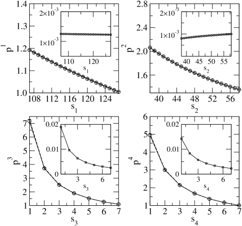
Figure 1: Approximate equilibrium densities. Starting from a community with 4 levels and occupancies $s_{1}=127$, $s_{2}=58$, $s_{3}=7$ and $s_{4}=7$, we plot the variation of $p^{\ell}$ as a function of $s_{\ell}$, which exhibits a dependence $C/s_{\ell}$. Full lines with circles show the exact solution of (13), and dotted lines with crosses show our approximation (26). Insets contain the relative error of each approximation. Remaining parameters are $R=1505$, $\gamma_{+}=0.5$, $\gamma_{-}=5$, $\rho=0.3$ and $\alpha=1$.

4.2 Approximation of the equilibrium abundances

In our model, each set $\{s_{\ell}\}_{\ell=0}^{L}$ of species occupancies in each level determines a set of equilibrium densities according to (13). Finding $p^{\ell}(\{s_{k}\})$ is difficult, but in this section we will give a rather good approximation for large enough $s_{\ell}$. First we write the system in terms of the total population at each level, $P^{\ell}=s_{\ell}p^{\ell}$ ($\ell=1,\dots,L$),

$$\begin{split}&\gamma_{+}P^{\ell-1}-\left(\rho+\frac{1-\rho}{s_{\ell}}\right)P^{\ell}-\gamma_{-}P^{\ell+1}=\alpha,\\ &P^{0}+\gamma_{-}P^{1}=R.\end{split}$$ (25)

Written in this way, it seems natural to expand the solution in powers of $1/s$. In B we show that we can approximate

$$P^{\ell}\approx\frac{T_{L,\ell}-(1-\rho)\sum_{k\neq\ell}^{L}Q_{L,\ell}^{k}/s_{k}}{D_{L}-(1-\rho)\sum_{k=1}^{L}B_{L,k}/s_{k}}.$$ (26)

As we can see in Figure 1, this first order approximation captures accurately the variation of the equilibrium densities $p^{\ell}$ with $s_{\ell}$. Besides, we also obtain a very accurate approximation when we vary the number of species $s_{j}$ in levels other than $\ell$. Note that, even when the occupancy of a level is small (lower panels of Figure 1), the approximation remains good.

In the limit $s_{\ell}\gg 1$ we obtain the dependence $p^{\ell}\approx C/s_{\ell}$, which provides the general tendency observed in Figure 1. Moreover, in the biologically relevant limit $R\gg\alpha$, and taking into account the explicit expressions for $T_{L,\ell}$ and $D_{L}$ given in B, populations behave like

$$p^{\ell}\approx\frac{R}{s_{\ell}}\left(\frac{\gamma_{+}}{\gamma_{-}}\right)^{\ell}\frac{a_{L-\ell}}{a_{L}+\gamma_{+}a_{L-1}}$$ (27)

for $\ell\geq 0$. Several conclusions can be extracted from this dependence. First, when the number of species in the $\ell$-th level is exhausted, according to (23), we obtain a population density $p^{\ell}\approx n_{c}$, as expected. But more importantly, it represents another reason for the extinction threshold to be included in our model. If there were no threshold, equilibrium densities would monotonically decrease with $s^{\ell}$ without ever becoming zero. The assembly graph would then contain infinitely many communities thus becoming intractable.

5 Invaded dynamics

In Capitán et al. (2009) it was assumed that, during the assembly process, successional invasions occur and modify resident communities at equilibrium. There we made the hypothesis of the average time between consecutive invasions being much longer than the typical dynamic time scale for the community to reach the equilibrium state. This is actually what is observed. In relation to the different time scales between invasion and competition, invasion events may take place at the scale of decades, long enough time for invaded communities to stabilize [for example, the rate of new invasions in islands may be one every few year (Sax et al., 2005)]. This assumption has also been made in previous papers like Kokkoris et al. (1999), where authors assume that after each invasion there is a re-organization of the community prior to a new invasion. Specifically, they solve the dynamical system describing the new community with the invader until reaching the carrying capacity. These new densities are then used as initial values for the new systems resulting from the next invasion [see details in Kokkoris et al. (1999)]. The same idea was applied in the construction of our assembly model (Capitán et al., 2009).

We used a second hypothesis as well, namely that the population of the invader is small (equal to the extinction threshold $n_{c}$). This is what is actually found in real situations. It is a well established fact that colonizers rarely reach a new habitat in high numbers (Roughgarden, 1974; Turelli, 1981). In theory, the probability of a small propagule to extend is used as the invasibility criterion. In biological control, management of invasions is based on looking for a small density of species in new areas (Liebhold and Bascompte, 2003). In this case, theoretical and empirical work has taken advantage to predict conditions of eradication based on density thresholds (Allee effects) and demographic stochasticity.

Therefore we can assume invaders arriving at some level of a community in equilibrium with a small abundance set equal to the extinction threshold. Under the species symmetry assumption, the dynamic system $\dot{n}_{i}^{\ell}=n_{i}^{\ell}q_{i}^{\ell}$ given by the response function (12) applies as well for the invaded system, with $N^{\ell}=\sum_{i=1}^{s_{\ell}}n_{i}^{\ell}+n$ and $n$ being the population density of the invader. Therefore, once the equilibrium is reached after the invasion, the density of the invader will equal $p^{\ell}$ (the density of the remaining species in that level), which can be obtained by solving (15) with an occupancy $s_{\ell}+1$ in the $\ell$-th level. Moreover, the global stability condition applies as well to the invaded dynamics. So we just need to check the viability of the resulting equilibria in order to determine whether the invader is accepted.

If the invasion takes place at level $L+1$, the equation for the invader is simply

$$\frac{\dot{n}}{n}=-\alpha+\gamma_{+}s_{L}n^{L}-n,$$ (28)

which in fact is the last equation of the system (15) for a community of $L+1$ levels with occupancies $\{s_{1},\dots,s_{L},1\}$. Hence the global stability condition still remains applicable and the invader will be accepted if the resulting equilibrium is viable.

The complexity of the assembly dynamics comes from the cases where some level in the invaded community falls below the extinction threshold. The approach we used in Capitán et al. (2009) to determine the sequence in which species go extinct until leading to a final viable ecosystem was the following: for the levels that fell below the extinction threshold once the equilibrium had been reached, we went back in their trajectory to the point where the population of some species crossed the extinction level $n_{c}$ for the first time, we eliminated one species from that level and restarted the dynamics from that point. In this paper we will propose an alternative way to determine that sequence based on several criteria and analytical approximations that we will discuss below.

5.1 Invasion criteria

Consider the general dynamical system $\dot{x}_{i}/x_{i}=q_{i}(x,x_{I})$, $\dot{x}_{I}/x_{I}=q_{I}(x,x_{I})$ for an arbitrary community with $S$ species, where $x$ are the densities of the species in the resident community and $x_{I}$ is the density of the invader. The establishment of a colonizer in systems of this kind depends crucially on the initial per-capita growth rate of the invader (Law and Morton, 1996). In fact, the condition that must be satisfied for a new species to increase when rare is

$$\lim_{T\rightarrow\infty}\frac{1}{T}\int_{0}^{T}q_{I}(\hat{x}(t),x_{I}=0)dt>0,$$ (29)

i.e., the time average of the per-capita rate of increase of the invader is positive when the species of the resident community remain under certain attractor $\hat{x}(t)$ of the dynamics. In our model, the only attractor is the interior rest point, so the condition reduces to $q_{I}(p,0)>0$, where $p$ is the rest point of the resident community. Strictly speaking, our model has a non-zero extinction threshold, so this condition has to be replaced by $q_{I}(p,n_{c})>0$. Since we start from a resident community initially at equilibrium and the invader initial density is $n_{c}$, this condition reduces to the initial per-capita growth rate of the invader.

The condition $q_{I}(p,n_{c})>0$ can be used to obtain criteria for the invasibility at each level. For example, consider the initial growth rate of the invader when the invasion takes place at the level $L+1$ [Eq. (28)]. The condition for this rate to be positive is

$$p^{L}>\frac{\alpha+n_{c}}{\gamma_{+}s_{L}}.$$ (30)

If this condition does not hold, the invader is the first species to go extinct because it starts at the extinction level and with a negative initial rate. In the end states, the populations of the resident community are close to (but above) $n_{c}$ (Capitán et al., 2009), so the former condition provides the approximate bound

$$s_{L}\geq\frac{\alpha+n_{c}}{\gamma_{+}n_{c}}.$$ (31)

Even if the initial growth rate of the invader is positive, asymptotically the level $L+1$ may not be viable. If this happens, during the time when the population of the invader is above $n_{c}$, extinctions may occur at lower levels. This situation explains the accumulation of recurrent states that we observed in Capitán et al. (2009) when we varied the resource saturation (see Section 6).

Invasions at levels $\ell\leq L$ are subject to similar conditions. For the initial growth rate of the invader to be positive

$$p^{\ell}>\frac{n_{c}}{1-\rho}$$ (32)

must hold. In general, an initially positive growth rate could lead to potential extinctions in the remaining levels while the equilibrium density of the invader is above the threshold. But it could happen as well that the invader extinguishes at equilibrium with some initial transient time above the extinction. To estimate a condition for this to happen, let us assume that densities and occupancies are inversely proportional (see (26) and Figure 1). Then the equilibrium abundance of the invader is $s_{\ell}p^{\ell}/(s_{\ell}+1)$, therefore if

$$p^{\ell}<n_{c}\left(1+\frac{1}{s_{\ell}}\right)$$ (33)

the invader goes extinct. This condition, together with (32), leads to

$$s_{\ell}<\frac{1}{\rho}-1$$ (34)

so below this bound, the invader initially grows but becomes extinct at equilibrium. We will use this condition to explain the appearance of some recurrent subsets for certain values of $R$ (see Section 6).

It would be nice, however, to have a systematic way to predict the sequence of extinctions after an invasion has occurred. Based on our approximations for the equilibrium densities, we can propose a way to sequentially remove species for invasions at lower levels. Within the end states of our model, abundances are close to the extinction threshold. Then (23) implies that communities are pyramidal, so lower levels are highly occupied but higher levels contain a small number of species. Accordingly, the increase of one species in a lower level has no significant effect in the equilibrium abundances of the community. Therefore if a species goes extinct after an invasion in a low level, it has to be the invader itself.

The extinction sequence for invasions in higher levels is not so easy to predict. Nevertheless, changes in abundances upon increasing $s_{\ell}$ are larger the higher the level (Figure 1) so, in case that several levels fall below the threshold, we can make the assumption that it is always the “highest” species the one that goes extinct first. This procedure provides a certain sequence of extinctions whose accuracy will be checked in Section 6.

The prediction of the sequence of extinctions can be complicated when a top predator invades if the resource saturation values do not allow for $L+1$ levels. We have devised global approximations to the dynamics in this case to predict the order of extinctions without having to resort to the numerical integration of the system of differential equations, as we did in Capitán et al. (2009).

5.2 Global approximations to the dynamics invaded by a top predator

Our heuristic approximations to the time dynamics of the system (15) when an invader arrives at level $L+1$ are somehow inspired in the matching technique used to obtain analytic approximations to perturbed differential equations [see, for example Bender and Orszag (1984)]. First we calculate the equilibrium point $\{p^{\ell}\}_{\ell=0}^{L}$ by either solving (13) or using the approximations (26). Then we approximate $n^{L+1}(t)$ by the sum of its long-term dependence $n_{\rm lt}^{L+1}(t)$ (near equilibrium) plus a short-term behavior $n_{\rm st}^{L+1}(t)$. For the long term, a linear stability analysis shows that the solution exponentially decays towards the equilibrium point, so we will set

$$n_{\rm lt}^{L+1}(t)=p^{L+1}+e^{-\lambda t}[d_{0}\cos(\omega t)+d_{1}\sin(\omega t)]$$ (35)

where the eigenvalue of the linear stability matrix which is closest to zero is $-\lambda+i\omega$ ($\omega$ may be zero). The constants $d_{0}$ and $d_{1}$ remain undetermined for the moment.

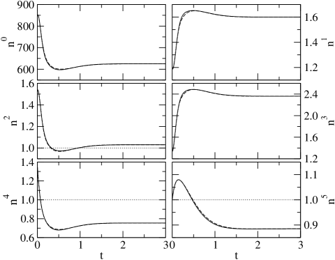
Figure 2: Dashed lines show our approximation for the dynamics of a four-level community determined by the occupancies $s_{1}=110$, $s_{2}=50$, $s_{3}=6$ and $s_{4}=5$ when invaded by a top predator at level $5$. For this case the eigenvalue closest to zero of the linear stability matrix is complex. Full lines represent the numerical integration of (12). Remaining parameters are the same as in Figure 1. The whole time evolution is accurately predicted. The extinction level $n_{c}=1$ is showed as a dotted line. We can see how the first extinction in the community takes place at level $4$.

For the short-term behavior we propose

$$n_{\rm st}^{L+1}(t)=C(t)e^{-\xi t},$$ (36)

where $C(t)=\sum_{j}c_{j}t^{j}$ is a polynomial whose coefficients and the exponent $\xi$ need to be determined to capture the transient time evolution. This way to express the short-term behavior is inspired in the initial transient decay that can be observed in the initial dynamics prior to getting close to the equilibrium point (see Figures 2 and 3). The polynomial has been included so as to properly capture the initial condition and the initial deviations to the exponential decay. The technical details to calculate the undetermined coefficients in (35) and (36) are deferred to C. Figures 2 and 3 illustrate the validity of this approximation in capturing the global trend of the time evolution.

To reproduce the ordering of the extinctions we need the extinction times for each level, and these times are approximated with a higher accuracy than the dynamic trajectories themselves (see Figure 3). In Figure 4 we illustrate, for a particular community, the extinction procedure compared to our analytical approximations. In this case, the first level falling below $n_{c}$ is the fourth one (upper panel). Then we remove one species from that level and restart the dynamics from the point of extinction, and the fourth level falls again below $n_{c}$ (second panel). After the removal of a new species, the fourth level ends up above $n_{c}$ at equilibrium. Now the next level ending below $n_{c}$ is the second one. We move to the point of extinction of this second level and restart the dynamics after removing one species from $\ell=2$. After that it is just the invader ($\ell=5$) the only one that falls below the threshold, so we remove it and the resulting community becomes viable. Were it not, we would apply the same extinction procedure again and again until the final community is viable. The sequence of extinctions is well reproduced with our approximate solution, although slight differences that alter the order of extinctions may occur when different levels fall below $n_{c}$ roughly at the same time.

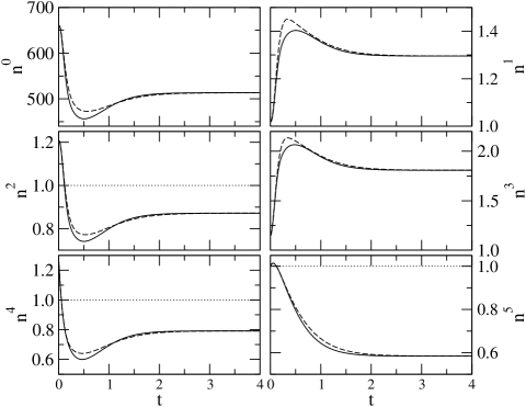
Figure 3: Same as Figure 2, but with $R=1200$ and occupancies $s_{1}=106$, $s_{2}=49$, $s_{3}=6$ and $s_{4}=4$. For this case the eigenvalue closest to zero of the linear stability matrix is real. Although there is some discrepancy in our approximations, the global trend is captured and the extinction times after the invasion are accurately predicted.

6 Application to community assembly

Our goal in this paper was to provide analytical support, albeit approximate, to the results obtained in Capitán et al. (2009). We want to check now whether our approximations correctly predict the recurrent sets which are end states of the assembly process. With this aim, we have varied the parameter $R$ within the range from 10 to 1700 in steps $\Delta R=5$. The remaining parameters of the model will be set as in our previous work: $\gamma_{+}=0.5$, $\gamma_{-}=5$, $\rho=0.3$, $\alpha=1$ and $n_{c}=1$.

Let us first fix the number of levels $L$. We can determine with (24) the minimum value $R_{\rm min}$ that allows $L+1$ levels. The results are summarized in Table 1. Moreover, we can combine (23) and (31) to give an estimation of the initial value of $R_{\rm rec}$ for the appearance of a recurrent set with more than one community,

$$\begin{split}\frac{R}{n_{c}}+\mu(\gamma_{-}+1)&\geq\left(\frac{\gamma_{-}}{\gamma_{+}}\right)^{L}\Biggl{[}\left(\frac{\alpha+n_{c}}{\gamma_{+}n_{c}}+\mu\right)(a_{L}+\gamma_{+}a_{L-1})\Biggr{.}\\ &+\Biggl{.}\mu(a_{L-1}+\gamma_{+}a_{L-2})\Biggr{]}.\end{split}$$ (37)

The resulting values show a good agreement with those obtained numerically in Capitán et al. (2009) (see Table 1).

$L$	$R_{\rm rec}/n_{c}$	$R^{*}_{\rm rec}/n_{c}$ $(\pm 5)$
1	25.80	$30$
2	75.88	$80$
3	323.93	$325$
4	973.56	$975$

$L$	$R_{\rm min}/n_{c}$	$R^{*}_{\rm min}/n_{c}$ $(\pm 5)$
2	35.80	$40$
3	131.88	$135$
4	457.53	$470$
5	1613.71	$1630$

Table 1: Estimation of the value of $R/n_{c}$ for the appearance of a recurrent set with more than one community (left). Minimum values of $R/n_{c}$ that allow a community with $L$ levels, according to (24) (right). The interval of values of $R$ that correspond to the recurrent sets is approximately $[R_{\rm rec},R_{\rm min}]$. $R^{*}_{\rm rec}$ and $R^{*}_{\rm min}$ are the corresponding values found using numerical analysis (Capitán et al., 2009) mapping the whole range of $R$ with a resolution $\Delta R=5$.

Then, for a given $R$, we can read off from Table 1 the number of levels for the communities within the recurrent set. Once we know it, we determine with (23) an estimation for the maximum occupancies allowed. We round off the estimates to get an integer set of values $\{s_{\ell}\}$ and calculate the associated interior equilibrium. It can happen that some of the $p^{\ell}$ fall below $n_{c}$, so we decrease the corresponding occupancies $s_{\ell}$ eliminating species one by one until the equilibrium turns out to be viable. This way we obtain a community very close to those of the recurrent set (communities within this set are close to extinction), so we can use it as the initial community to start the assembly process. We then compute the set of viable communities connected to it, which defines an assembly graph much smaller than those obtained in Capitán et al. (2009) starting from the empty community $\varnothing$. We analyze the graph to obtain its recurrent sets using the algorithm of Xie and Beerel (1998) and we get one single set. In Figures 5 and 6 we plot the number of communities in each end state, showing a good agreement between the results obtained with the analytical approximations reported here and the numerical results reported in Capitán et al. (2009).

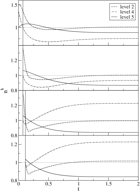
Figure 4: Extinctions sequence for the community with $s_{1}=110$, $s_{2}=51$, $s_{3}=6$ and $s_{4}=5$ invaded at level 5 (parameter values are the same as in Figure 1, and $n_{c}=1$ is showed with a horizontal dotted line). We just show the time evolution of the levels that go extinct or are close to extinction in equilibrium. Dotted curves correspond to our analytical approximations. We show, with vertical lines, the time of the first level that go extinct. The sequence of extinct levels is 4, 4, 2, 5 until viability is recovered.

For every $R$ we can always find a community which is uninvadable at all its levels $\ell\leq L$. If $R$ is such that (37) is not verified, then the invader at level $L+1$ initially decreases and goes extinct. This explains the intervals of $R$ where only one absorbent state is found. However, if (31) holds (with our choice of parameters this happens when $s_{L}\geq 4$), there is an initial time interval where the population of the invader is above the threshold. This can cause the extinction of lower level species, and generate recurrent sets with more than one community.

Our analytical approximations thus provide results very close to those obtained numerically. Besides its being more efficient (the whole assembly needs not be generated), this method also allows to predict what would happen for values of $R$ larger than 1700, which are computationally prohibitive for the numerical method. With our bounds (24) and (37) we can estimate the next interval of $R$ where more than one community in the end state will appear, namely $R\in[3844,5114]$. That is out of reach of the numerical method, because the number of communities in the whole assembly graph grows as fast as $N\approx e^{\kappa\sqrt{R}}$ (Capitán et al., 2010).

Two observations are on purpose. First, there are small intervals of $R$ where the graph constructed starting from the empty community has $L$ levels but there are viable communities with $L+1$ levels which cannot be assembled starting from $\varnothing$ [this phenomenon is analogous to the existence of unreachable persistent communities showed in Warren et al. (2003)]. We observe this for $R=$ 460, 465, 1615, 1620 and 1625 (see Table 1). We have checked that even in these cases the recurrent state is exactly recovered using the analytical approximations.

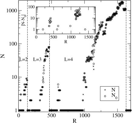
Figure 5: Number of communities in the recurrent sets obtained with the analytical approximations ($N$, showed with crosses) and with a numerical integration of the population dynamics ($N_{0}$, circles). The inset contains the absolute difference $|N-N_{0}|$. The global picture is the same as that found in Capitán et al. (2009), although differences of a few tens arise in some cases.

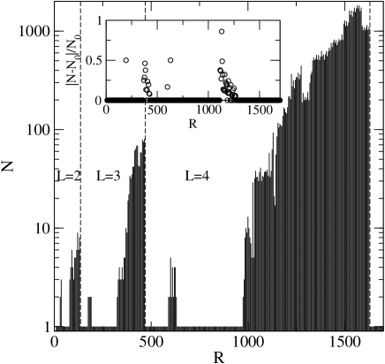
Figure 6: Number $N$ of communities in the recurrent sets obtained with the analytical approximations (crosses in Figure 5). The global trend is the same as found in our previous work [see Figure 3. in Capitán et al. (2009)]. The inset shows the relative difference in the prediction of the number of communities in the end states. Note that the discrepancies occur in a region where this number is small. This explains the relatively large error found in some cases.

Secondly, we can observe from Figures 5 and 6 that there are small regions where recurrent sets with more than one community are found out of the intervals predicted in Table 1 (around $R\approx 200$ for $L=3$ and $R\approx 620$ for $L=4$). For those values, a single absorbent community should be found. However, condition (34) for an invader at level $L$ to initially grow and become extinct at equilibrium renders $s_{L}\leq 2$ for our choice of $\rho$. We have checked that this condition is satisfied by all these small recurrent sets, thus explaining their appearance.

We have to assess the accuracy of the transitions predicted in the graph of our recurrent sets. Note that a slight difference in the ordering of extinctions can change the final community after the invasion and this may change the observed graph and therefore the asymptotic probability distribution of the associated Markov chain. In order to check the transition matrices we obtain, we have calculated two averages. In Figure 7 we show the variation of the average number of species in the recurrent sets as a function of $R$. The behavior is almost indistinguishable from that found in Capitán et al. (2009) (the inset of Figure 7 shows that the relative error is small).

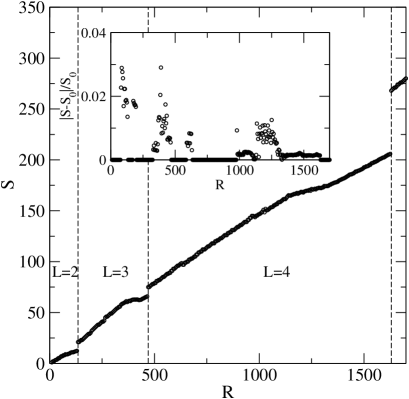
Figure 7: Average number of species $S_{\rm av}$ in the end states calculated analytically vs. $R$. In the inset we show the relative error between $S$ and its corresponding average $S_{0}$ for each graph calculated numerically.

We have also checked that the number of extinctions predicted with our approximations follows the same distribution than the one calculated numerically. To this purpose we define the magnitude of an avalanche of extinctions as the relative variation $m=\Delta S/S$ of the total number of species in a community after an invasion. In Figure 8 we show the cumulative histogram for the distribution of these magnitudes. We can see that the deviations between both distributions are small. Further statistical results will be discussed in the second paper of this suite.

7 Conclusions

In this paper we have presented a general model of trophic-level structured food-web, where interactions between species are either feeding or competing. For the sake of simplicity, feeding only takes place between contiguous levels. The population dynamics is modeled through Lotka-Volterra equations, and a proof is given that a wide class of these models has a globally stable interior equilibrium. We have introduced this model as an appropriate general framework to study the process of successional invasions. In the invasion process, we consider a mean-field version, in which species in the same level are trophically equivalent and only intra- and interspecific competition is distinguished. This species symmetry assumption has allowed us to obtain analytical results, some of them exact and some other approximate. Among them we have provided estimations for the maximum number of species allowed per level, the maximum number of levels for a given value of the resource saturation, and certain analytical approximations of the dependence of the equilibrium abundances on the occupancies of each level. We have combined these results with some criteria for the acceptance of an invader in our model communities, and with the help of some global approximations of the invaded dynamics we have been able to obtain, with high accuracy, the sequence of extinctions occurring after an invasion. With this procedure we have reproduced the same results that we found in a previous work (Capitán et al., 2009), this time without resorting to an integration of the Lotka-Volterra equations and without constructing the whole assembly graph. Among other things this brings the opportunity of exploring the model for resources which would otherwise be computationally prohibitive to obtain.

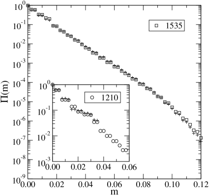
Figure 8: Cumulative probability function $\Pi(m)$ for the distribution of the magnitude $m$ of avalanches of extinctions. The distributions follow an exponential behavior. Crosses represent the results for our approximated transition matrix. The number of recurrent states coincide for the analytical and numerical method. The inset shows a case where the number of communities is underestimated. This explains the absence of several points in the distribution estimated analytically. The agreement is rather good even in this case.

Although the main results of this model are discussed at length in the second paper of this suite (Capitán et al., 2010), we have provided here a few of them which illustrate the global assembly process and some of its main features. For instance, we had reported already in Capitán et al. (2009) that, upon increasing the resource saturation $R$, the number of levels, $L$, that the system is able to sustain increases discontinuously. We provide here an estimate of the values of $R$ at which this occurs, and show that this values grow essentially as $\sim(\gamma_{+}/\gamma_{-})^{L}$. Under the assumption that populations are close to the extinction level, we have shown that equilibrium communities are pyramids —again in agreement with the results obtained in Capitán et al. (2009). Close to the onset of appearance of a new level, the number of communities in the end state increases. We have identified that the requirement for this to happen is that the population of a top predator invading the community initially grows only to go eventually extinct. From this knowledge we can estimate the value of $R$ at which the end state starts to have more than just one community.

We have tested the approximations we have made by calculating some observables. Among them we report on the average species richness as a function of $R$, as well as the distribution of the avalanche of extinctions produced by an invasion. In both cases the agreement is very good. In the latter case, it is worth mentioning that this distribution of avalanches decays exponentially with the avalanche size, meaning that there is a characteristic size of the avalanches. This size roughly grows with the species richness of the community, as one could expect. In any case, avalanches never get even close to destroy the community.

We also propose in this paper an analytical approximation to the dynamics of a community invaded by a top predator. This approximation has been built matching the initial behavior of the solution (derived from the initial condition) and the asymptotic decay expected close to the equilibrium. We have found a a rather good agreement with the solutions obtained by a numerical integration of the Lotka-Volterra equations, and has allowed us to correctly predict (in most of the cases) the order of extinctions eventually caused by the invasion of a top predator. These approximations have been applied to reproduce the assembly graphs for the recurrent sets, showing small discrepancies only for certain values of $R$. This provides an alternative method to analyze the system for other sets of parameter values, with a negligible computational cost compared to the construction of the whole assembly graph.

Our assembly model is based on several assumptions regarding the invasion process. Two of the most important ones are that newcomers invade at low population and the average time between invasions is large compared to the time for the communities to reach the equilibrium. If the invasion rate is too high (Fukami, 2004; Bastolla et al., 2005b) or if the invasion is not produced by rare species (Hewitt and Huxel, 2002), the assembly process —and hence the resulting end states— can be drastically altered. The reason is that communities that are not accessible from the equilibrium state may be so from a transient or if there is a massive invasion. This changes the assembly graph in ways that we can neither predict nor even check, because these processes are out of reach of our model. For instance, considering invading transients, one of the strong simplifications we make use of is that of starting always from a well-defined initial condition, namely the equilibrium state. If the system can be invaded at any moment during a transient there are infinitely many initial conditions to start off from, something we cannot implement. So what happens if any of those two hypotheses is violated remains an open question.

8 Acknowledgements

This work is funded by projects MOSAICO, from Ministerio de Educación y Ciencia (Spain) and MODELICO-CM, from Comunidad Autónoma de Madrid (Spain). The first author also acknowledges financial support through a contract from Consejería de Educación of Comunidad de Madrid and Fondo Social Europeo.

Appendix A Derivation of the reduced dynamical system

We will show in this appendix that our dynamical system $\dot{n}_{i}^{\ell}=q_{i}^{\ell}n_{i}^{\ell}$, with the linear response function (12), can be reduced to the form (15) when all the initial species abundances at a certain level are equal. The crucial point for this to be true is the relation (14).

This result can be formulated in a simple way. Consider the two-dimensional autonomous system

$$\begin{split}\dot{x}&=f(x,y),\\ \dot{y}&=g(x,y),\end{split}$$ (38)

with the initial condition $x(0)=y(0)$ and which satisfies $f(x,y)=g(y,x)$. We are going to show that the Taylor expansions centered at $t=0$ of $x$ and $y$ are identical. In principle, both expansions will have certain radii of convergence. Let $t$ be lower than the minimum of these radii. Then we just need to show that all the derivatives at $t=0$ coincide. But this follows by induction.

The first derivatives are shown to be equal easily. Let us assume that $x^{(k)}(0)=y^{(k)}(0)$ for all $k=1,\dots,n$. Then the $(n+1)$-th derivative is

$$x^{(n+1)}(0)=\sum_{j=0}^{n}\left(\begin{array}[]{c}n\\ j\end{array}\right)\left.\frac{\partial^{n}f}{\partial x^{j}\partial y^{n-j}}\right|_{t=0}x^{(j)}(0)y^{(n-j)}(0).$$ (39)

But, since $f(x,y)=g(y,x)$, this is equivalent to write

$$x^{(n+1)}(0)=\sum_{j=0}^{n}\left(\begin{array}[]{c}n\\ j\end{array}\right)\left.\frac{\partial^{n}g}{\partial y^{j}\partial x^{n-j}}\right|_{t=0}y^{(j)}(0)x^{(n-j)}(0),$$ (40)

and, relabelling the sum index,

$$x^{(n+1)}(0)=\sum_{j=0}^{n}\left(\begin{array}[]{c}n\\ n-j\end{array}\right)\left.\frac{\partial^{n}g}{\partial x^{j}\partial y^{n-j}}\right|_{t=0}x^{(j)}(0)y^{(n-j)}(0),$$ (41)

which is equal to $y^{(n+1)}(0)$.

Therefore we have shown that the Taylor expansions of $x(t)$ and $y(t)$ coincide. This means that $x(t)=y(t)$ within the radius of convergence of the series. For larger times, we can apply the same argument by analytic continuation (we choose some $t_{0}$ in the interval or convergence as the centering point for a new Taylor expansion, and repeat the argument). Hence we conclude that $x(t)=y(t)$ for all $t$.

Note that the same considerations apply to our system (12), so we can reduce considerably the complexity of the system and solve (15) instead.

Appendix B Analytical approximation to the equilibrium densities

This appendix is devoted to solve the linear system for the equilibrium densities (25). The solution of this system can be obtained through Cramer’s rule as

$$s_{\ell}p^{\ell}=\frac{\Xi_{L,\ell}}{\Delta_{L}}$$ (42)

for certain determinants $\Xi_{L,\ell}$ and $\Delta_{L}$. Our approximation is based in some recurrent equations that can be obtained for these determinants.

Let us start with the $(L+1)\times(L+1)$ determinant

$$\Delta_{L}=\begin{array}[]{|ccccc|}-1&-\gamma_{-}&0&\cdots&0\\ \gamma_{+}&-d_{1}&-\gamma_{-}&\cdots&0\\ 0&\gamma_{+}&-d_{2}&\cdots&0\\ \vdots&\vdots&\vdots&&\vdots\\ 0&0&0&\cdots&-d_{L}\end{array},$$ (43)

where $d_{\ell}\equiv\rho+\frac{1-\rho}{s_{\ell}}$. Hence the densities depend on $\{s_{\ell}\}_{\ell=1}^{L}$ only through the inverse of all the possible products $s_{i_{1}}s_{i_{2}}\cdots s_{i_{k}}$, for some combination $(i_{1},i_{2},\dots,i_{k})$ of $k$ elements of the set $\{1,2,\dots,L\}$. In the recurrent sets we get the highest occupancy of species in each level allowed by the resource according to (21)–(23), so we expect that a rather good approximation for the equilibrium densities amounts to neglecting orders higher than $1/s$. Hence

$$\Delta_{L}=D_{L}-(1-\rho)\sum_{\ell=1}^{L}\frac{B_{L,\ell}}{s_{\ell}}+\mathcal{O}\left(\frac{1}{s^{2}}\right),$$ (44)

where

$$D_{L}=\begin{array}[]{|ccccc|}-1&-\gamma_{-}&0&\cdots&0\\ \gamma_{+}&-\rho&-\gamma_{-}&\cdots&0\\ 0&\gamma_{+}&-\rho&\cdots&0\\ \vdots&\vdots&\vdots&&\vdots\\ 0&0&0&\cdots&-\rho\end{array}$$ (45)

has dimension $(L+1)\times(L+1)$ and $B_{L,\ell}$ is the determinant obtained by substituting the $\ell$-th column of $D_{L}$ by the column vector $u_{\ell}$ whose components are $u_{\ell,i}=\delta_{\ell,i}$ (for $i=0,1,\dots L$).

The determinant $D_{\ell}$ satisfies the recursion

$$D_{\ell}=-\rho D_{\ell-1}+\gamma_{+}\gamma_{-}D_{\ell-2},$$ (46)

where $\ell=1,2,\dots L$, $D_{0}=-1$ and $D_{1}=\rho+\gamma_{+}\gamma_{-}$. This relation can be easily solved using a generating function. On the other hand, it is easy to see that $B_{L,\ell}=D_{\ell-1}E_{L-\ell-1}$, with $E_{\ell}$ the $(\ell+1)\times(\ell+1)$ determinant

$$E_{\ell}=\begin{array}[]{|ccccc|}-\rho&-\gamma_{-}&0&\cdots&0\\ \gamma_{+}&-\rho&-\gamma_{-}&\cdots&0\\ 0&\gamma_{+}&-\rho&\cdots&0\\ \vdots&\vdots&\vdots&&\vdots\\ 0&0&0&\cdots&-\rho\end{array},$$ (47)

which also satisfies recursion (46) with $E_{0}=-\rho$ and $E_{1}=\rho^{2}+\gamma_{+}\gamma_{-}$.

The generating function that results from (46) is

$$G(z)=\sum_{\ell=0}^{\infty}D_{\ell}z^{\ell}=\frac{D_{0}+(D_{1}+\rho D_{0})z}{\gamma_{+}\gamma_{-}z^{2}-\rho z-1},$$ (48)

and after the series expansion we get

$$D_{\ell}=(-\gamma_{-})^{\ell-1}\left[(D_{1}+\rho D_{0})a_{\ell-1}-\gamma_{-}E_{0}a_{\ell}\right],$$ (49)

with $a_{\ell}$ given by (18). Then the following compact expressions result

$$D_{\ell} =(-1)^{\ell+1}\gamma_{-}^{\ell}\left[a_{\ell}+\gamma_{+}a_{\ell-1}\right],$$ (50)

$$E_{\ell} =(-1)^{\ell+1}\gamma_{-}^{\ell+1}a_{\ell+1}.$$ (51)

The explicit expression for $\Xi_{L,\ell}$ is obtained from $\Delta_{L}$ substituting its $\ell$-th column by the $(L+1)\times 1$ column vector $(-R,\alpha,\dots,\alpha)^{\rm T}$. We can expand it up to leading order in powers of $1/s$ to get

$$\Xi_{L,\ell}=T_{L,\ell}-(1-\rho)\sum_{\begin{subarray}{c}j=1\\ j\neq\ell\end{subarray}}^{L}\frac{Q_{L,\ell}^{j}}{s_{j}}+\mathcal{O}\left(\frac{1}{s^{2}}\right).$$ (52)

where

$$T_{L,\ell} =\begin{array}[]{|ccccccc|}-1&-\gamma_{-}&0&\cdots&-R&\cdots&0\\ \gamma_{+}&-\rho&-\gamma_{-}&\cdots&\alpha&\cdots&0\\ 0&\gamma_{+}&-\rho&\cdots&\alpha&\cdots&0\\ \vdots&\vdots&\vdots&&\vdots&&\vdots\\ 0&0&0&\cdots&\alpha&\cdots&-\rho\end{array}$$ (58)

$$\hskip 11.95013pt\begin{array}[]{ccccccc}(0)&\phantom{-\gamma_{-}}&\phantom{-\gamma_{-}}&\phantom{\,\cdots}&(\ell)&\phantom{\,\cdots}&(L)\\ \end{array}$$ (60)

and $Q_{L,\ell}^{j}$ is the determinant that results when we substitute the $j$-th column of $T_{L,\ell}$ by $u_{j}$ ($j\neq\ell$).

Expanding $T_{L,\ell}$ along its first row we get

$$T_{L,\ell}=-\alpha A_{L,\ell}+\alpha\gamma_{+}\gamma_{-}A_{L-1,\ell-1}+(-1)^{\ell+1}R\gamma_{+}^{\ell}E_{L-\ell-1},$$ (61)

where we define the new $i\times i$ determinants $A_{i,j}$ as

$$A_{i,j} =\begin{array}[]{|ccccccc|}-\rho&-\gamma_{-}&0&\cdots&1&\cdots&0\\ \gamma_{+}&-\rho&-\gamma_{-}&\cdots&1&\cdots&0\\ 0&\gamma_{+}&-\rho&\cdots&1&\cdots&0\\ \vdots&\vdots&\vdots&&\vdots&&\vdots\\ 0&0&0&\cdots&1&\cdots&-\rho\end{array}$$ (67)

$$\hskip 11.95013pt\begin{array}[]{ccccccc}(1)&\phantom{-\gamma_{-}}&\phantom{-\gamma_{-}}&\phantom{\cdots}&(j)&\phantom{\cdots}&(i)\\ \end{array}$$ (69)

that satisfy the recurrence equation

$$A_{n,j}=-\rho A_{n-1,j}+\gamma_{+}\gamma_{-}A_{n-2,j}+\gamma_{-}^{n-j}E_{j-2},$$ (70)

for $j=1,2,\dots,n-1$ (with the boundary conditions $A_{j,j+1}=0$ and $A_{j,0}=0$), and

$$A_{n,n}=-\gamma_{+}A_{n-1,n-1}+E_{n-2}.$$ (71)

These relations can be explicitly solved. On the one hand, by definition $A_{1,1}=1$, which amounts to choosing $E_{-1}\equiv 1$ for this to be compatible with (71). Moreover, making use again of a generating function, the solution of (71) is

$$A_{j,j}=\frac{(-1)^{j-1}\gamma_{-}^{j}}{\gamma_{-}-\gamma_{+}+\rho}\left[\frac{\rho}{\gamma_{-}}a_{j-1}+\frac{\gamma_{+}+\rho}{\gamma_{-}}a_{j-2}+\frac{\gamma_{+}}{\gamma_{-}}a_{j-3}-\left(\frac{\gamma_{+}}{\gamma_{-}}\right)^{j}\right],$$ (72)

for $j\geq 2$. On the other hand, the explicit solution of (70) is

$$\begin{split}A_{j+k,j}&=(-1)^{k}\gamma_{-}^{k+1}a_{k+1}A_{j,j}\\ &+\frac{\gamma_{-}^{k}E_{j-2}}{\gamma_{-}-\gamma_{+}+\rho}\left[(-1)^{k+1}(\gamma_{-}a_{k}-\gamma_{+}a_{k-1})+\gamma_{-}\right],\end{split}$$ (73)

for $k\geq 1$. Therefore equations (72) and (73), together with (61), provide an explicit solution for the determinants $T_{L,\ell}$.

Fortunately, $Q_{L,\ell}^{j}$ can be written in terms of the previous determinants since $Q_{L,\ell}$ is a block-diagonal determinant with two blocks that satisfies

$$Q_{L,\ell}^{j} =D_{j-1}A_{L-\ell,\ell-j},\quad\textrm{for}\quad k<j,$$ (74)

$$Q_{L,\ell}^{j} =E_{L-j-1}T_{j-1,\ell},\quad\,\textrm{for}\quad k>j.$$ (75)

This completes the analytical approximation of the equilibrium densities of our dynamical model. We have derived explicit expressions for all the terms involved in (42), (44) and (52) up to leading order in $1/s$. Moreover, note that the same technique applied to find this approximation can be extended to obtain the exact dependence on $\{s_{\ell}\}_{\ell=1}^{L}$ of the abundances. Higher-order terms in powers of $1/s$ introduce in the corresponding determinants several column vectors of the type of $u_{\ell}$ making each determinant to be block-diagonal involving $D_{\ell}$, $E_{\ell}$, $A_{i,j}$ or $T_{\ell,k}^{j}$, so that the general solution contains in each term a product of a certain combination of these determinants. This explicit expression can in fact be written, but it is too cumbersome. The approximations here obtained are both sufficiently simple and accurate enough to capture the behavior of population densities in the communities of the recurrent sets.

Appendix C Technical details of the global approximations to the dynamics

In this appendix we will describe the calculation of the undetermined parameters of our ansatz (35)–(36) for the dynamics of system invaded by a top predator. We impose that the initial condition and the first $k$ derivatives at $t=0$ match the exact values, which can be readily calculated. Indeed, our system has the form $\dot{x}_{i}=-\alpha x_{i}+x_{i}f_{i}(x)$, where $f_{i}(x)=\sum_{j}b_{ij}x_{j}$ is a linear function. Therefore we can recursively calculate the $s+1$ initial derivative as

$$x^{(s+1)}_{i}(0)=-\alpha x^{(s)}_{i}(0)+\sum_{j=0}^{s}\left(\begin{array}[]{c}s\\ j\end{array}\right)x^{(s-j)}_{i}(0)f_{i}(x^{(j)}(0)).$$ (76)

For a real eigenvalue ($\omega=0$), we choose $C(t)$ [see (36)] to be a polynomial of degree $k-2$, and for a complex one ($\omega\neq 0$) we choose degree $k-3$, in order to compensate for the extra undetermined coefficient in the long-term behavior in this case. Equating the approximate solution to the initial condition and the first $k-1$ derivatives of our ansatz to the exact values leads to a linear system for the undetermined coefficients. The equation for the $k$-th derivative yields a polynomial equation for $\xi$, namely

$$\sum_{j=0}^{k-2}\left(\begin{array}[]{c}k-2\\ j\end{array}\right)H_{j}\xi^{k-j-2}=(\lambda^{2}+\omega^{2})p^{L+1},$$ (77)

when $\omega=0$, where

$$H_{j}=(\lambda^{2}+\omega^{2})n^{(j)}(0)+2\lambda n^{(j+1)}(0)+n^{(j+2)}(0)$$ (78)

and $n^{(j)}$ stands for the $j$-th derivative of $n^{L+1}$, which can be calculated exactly using (76). For $\omega=0$ Eq. (77) gets replaced by

$$\sum_{j=0}^{k-1}\left(\begin{array}[]{c}k-1\\ j\end{array}\right)\left[\lambda n^{(j)}(0)+n^{(j+1)}(0)\right]\xi^{k-j-1}=\lambda p^{L+1}.$$ (79)

Afterwards, we just need to calculate the coefficients $c_{j}$ and $d_{0}$ (and $d_{1}$, if $\omega\neq 0$) by solving the linear system that they satisfy.

Once we have the approximate time behavior for $n^{L+1}$ we calculate analytically the remaining populations $n^{\ell}$ by direct substitution into the system (15), taking advantage of the recursive form of these equations, once $n^{L+1}$ is known. Notice that, since we have to calculate successive derivatives in order to get any lower population, the accuracy of $n^{L+1}$ at short times degrades as we calculate lower level populations. Fortunately the model produces communities with a small number of trophic levels (Capitán et al., 2009). The choice $k=5$ seems to be enough to account for the dynamics of any community of up to $L=4$ levels invaded by a top predator (see Figures 2 and 3). For the description of the dynamics of communities with a higher number of levels we would need to choose polynomials of higher degree in our ansatz.

A final caveat needs to be made with respect to the calculation of $\xi$. We need it to be positive, otherwise (36) would be meaningless. Among all the roots of (77) we choose the largest, positive, real solution, so that any possible initial oscillation of the polynomial $C(t)$ is damped by the exponential. In the majority of the dynamics that we have approximated (see Section 6), we are able to find a positive solution for $\xi$. However, in some cases there is no positive solution. In those cases we just minimize the difference between the exact $k$-th derivative and the approximate one at $t=0$. This also produces an acceptable solution. In all minimization procedures that we have run, a positive exponent $\xi$ is always found.

References

- Alonso et al. (2008) Alonso, D., Ostling, A., Etienne, R.S., 2008. The implicit assumption of symmetry and the species abundance distribution. Ecol. Let. 11, 93–105.
- Bascompte and Melián (2005) Bascompte, J., Melián, C.J., 2005. Simple trophic modules for complex food webs. Ecology 86, 2868–2873.
- Bastolla et al. (2005a) Bastolla, U., Lässig, M., Manrubia, S.C., Valleriani, A., 2005a. Biodiversity in model ecosystems, i: coexistence conditions for competing species. J. Theor. Biol. 235, 521–530.
- Bastolla et al. (2005b) Bastolla, U., Lässig, M., Manrubia, S.C., Valleriani, A., 2005b. Biodiversity in model ecosystems, ii: species assembly and food web structure. J. Theor. Biol. 235, 531–539.
- Bender and Orszag (1984) Bender, C.M., Orszag, S.A., 1984. Advanced mathematical methods for scientists and engineers. McGraw–Hill, Singapore.
- Borrvall et al. (2000) Borrvall, C., Ebenman, B., Jonsson, T., 2000. Biodiversity lessens the risk of cascading extinction in model food webs. Ecol. Lett. 3, 131–136.
- Capitán et al. (2009) Capitán, J.A., Cuesta, J.A., Bascompte, J., 2009. Statistical mechanics of ecosystem assembly. Physical Review Letters 103, 168101–4.
- Capitán et al. (2010) Capitán, J.A., Cuesta, J.A., Bascompte, J., 2010. Species assembly in model ecosystems, ii: Results of the assembly process .
- Case (1990) Case, T.J., 1990. Invasion resistance arises in strongly interacting species-rich model competition communities. Proc. Natl. Acad. Sci. USA 87, 9610–9614.
- Case (1991) Case, T.J., 1991. Invasion resistance, species build-up and community collapse in metapopulation models with interspecies competition. Biol. J. Linn. Soc. 42, 239–266.
- Drake (1990) Drake, J.A., 1990. The mechanics of community assembly and succession. J. Theor. Biol. 147, 213–233.
- Dunne (2006) Dunne, J.A., 2006. The network structure of food webs, in: Pascual, M., Dunne, J.A. (Eds.), Ecological Networks. Oxford University Press, Oxford, pp. 27–86.
- Eklöf and Ebenman (2006) Eklöf, A., Ebenman, B., 2006. Species loss and secondary extinctions in simple and complex model communities. J. Anim. Ecol. 75, 239–246.
- Elton (1958) Elton, C.S., 1958. Ecology of invasions by animals and plants. Chapmann & Hall, London.
- Etienne and Alonso (2007) Etienne, R.S., Alonso, D., 2007. Neutral community theory: how stochasticity and dispersal-limitation can explain species coexistence. J. Stat. Phys. 128, 485–510.
- Fukami (2004) Fukami, T., 2004. Community assembly along a species pool gradient: implications for multiple-scale patterns of species diversity. Popul. Ecol. 46, 137–147.
- Fukami and Morin (2003) Fukami, T., Morin, P.J., 2003. Productivity-biodiversity relationships depend on the history of community assembly. Science 424, 423–426.
- Hewitt and Huxel (2002) Hewitt, C.L., Huxel, G.R., 2002. Invasion success and community resistance in single and multiple species invasion models: do the models support the conclusions? Biol. Inv. 4, 263–271.
- Hofbauer and Sigmund (1998) Hofbauer, J., Sigmund, K., 1998. Evolutionary games and population dynamics. Cambridge University Press, Cambridge.
- Huang (1987) Huang, K., 1987. Statistical Mechanics. Wiley, New York.
- Hubbell (2001) Hubbell, S.P., 2001. The Unified Theory of Biodiversity and Biogeography. Princeton University Press, Princeton.
- Karlin and Taylor (1975) Karlin, S., Taylor, H.M., 1975. A first course in stochastic processes. Academic Press, New York.
- Kokkoris et al. (1999) Kokkoris, G.D., Troumbis, A.Y., Lawton, J.H., 1999. Patterns of species interaction strength in assembled theoretical competition communities. Ecol. Lett. 2, 70–74.
- Lässig et al. (2001) Lässig, M., Bastolla, U., Manrubia, S.C., Valleriani, A., 2001. Shape of ecological networks. Phys. Rev. Lett. 86, 4418–4421.
- Law (1999) Law, R., 1999. Theoretical aspects of community assembly. In: Advanced ecological theory (ed. J. McGlade). Blackwell Science, Oxford.
- Law and Morton (1993) Law, R., Morton, R.D., 1993. Alternative permanent states of ecological communities. Ecology 74, 1347–1361.
- Law and Morton (1996) Law, R., Morton, R.D., 1996. Permanence and the assembly of ecological communities. Ecology 77, 762–775.
- Levine and D’Antonio (1999) Levine, J.M., D’Antonio, C.M., 1999. Elton revisited: a review of evidence linking diversity and invasibility. Oikos 87, 15–26.
- Lewis and Law (2007) Lewis, H.M., Law, R., 2007. Effects of dynamics on ecological networks. J. Theor. Biol. 247, 64–76.
- Liebhold and Bascompte (2003) Liebhold, A.M., Bascompte, J., 2003. The allee effect, stochastic dynamics and the eradication of alien species. Ecol. Lett. 6, 133–140.
- MacArthur (1955) MacArthur, R.H., 1955. Fluctuations of animals populations and a measure of community stability. Ecology 36, 533–536.
- MacArthur and Levins (1964) MacArthur, R.H., Levins, R., 1964. Competition, habitat selection, and character displacement in a patchy environment. Proc. Natl. Acad. Sci. 51, 1207–1210.
- Martinez et al. (2006) Martinez, N.D., Williams, R.J., Dunne, J.A., 2006. Diversity, complexity and persistence in large model ecosystems, in: Pascual, M., Dunne, J.A. (Eds.), Ecological Networks. Oxford University Press, Oxford, pp. 163–186.
- May (1972) May, R.M., 1972. Will a large complex system be stable? Nature 238, 413–414.
- May (1973) May, R.M., 1973. Stability and complexity in model ecosystems. Princeton University Press, Princeton.
- McCann (2000) McCann, K.S., 2000. The diversity-stability debate. Nature 405, 228–233.
- Morton and Law (1997) Morton, R.D., Law, R., 1997. Regional species pools and the assembly of local ecological communities. J. Theor. Biol. 187, 321–331.
- Odum (1953) Odum, E.P., 1953. Fundamentals of ecology. Saunders, Philadelphia.
- Pimm (1982) Pimm, S.L., 1982. Food webs. Chapman & Hall, London.
- Pimm (1991) Pimm, S.L., 1991. The balance of nature: Ecological issues in the conservation of species and communities. University of Chicago Press, Chicago.
- Post and Pimm (1983) Post, W.M., Pimm, S.L., 1983. Community assembly and food web stability. Math. Biosc. 64, 169–192.
- Rezende et al. (2007) Rezende, E., Lavabre, J., aes, P.G., Jordano, P., Bascompte, J., 2007. Non-random coextinctions in phylogenetically structured mutualistic networks. Nature 448, 925–929.
- Roughgarden (1974) Roughgarden, J., 1974. Scpecies packing and the competition function with illustrations form coral reef fish. Theor. Population Biol. 5, 163–186.
- Sax et al. (2005) Sax, D.F., Stachowicz, J.J., Gaines, S.D. (Eds.), 2005. Species Invasions: Insights into Ecology, Evolution, and Biogeography, Sinauer Associates Inc., Sunderland, Massachusetts.
- Turelli (1981) Turelli, M., 1981. Niche overlap and invasion of competitors in random evironments i: models without demographic stichaticity. Theor. Population Biol. 20, 1–56.
- Warren et al. (2003) Warren, P.H., Law, R., Weatherby, A.J., 2003. Mapping the assembly of protist communities in microcosms. Ecology 84, 1001–1011.
- Xie and Beerel (1998) Xie, A., Beerel, P.A., 1998. Efficient state classification of finite-state markov chains. IEEE T. Comput. Aid. D. 17, 1334–1339.