Superluminal, subluminal, and negative velocities in free-space electromagnetic propagation

Abstract

In this Chapter the time-domain analysis of the velocity of the electromagnetic field pulses generated by a spatially compact source in free space is presented. Recent simulations and measurements of anomalous superluminal, subluminal, and negative velocities are discussed. It is shown that such velocities are local and instantaneous in nature and do not violate either causality or special relativity. Although these effects are mainly confined to the near- and intermediate-field zones, some of them seem paradoxical and still lack adequate physical interpretation.

1 Introduction

Historically, the fact that the electromagnetic field propagates in vacuum with the speed of light $c=299792458$ m/s was used to establish the electromagnetic (wave) nature of light and the correctness of Maxwell’s equations. The invariance of the speed of light with respect to inertial reference frames has lead to the special relativity theory and its idea of space-time and was used to fix the standard of length once and for all, Giacomo (1984). The realization that nothing can travel faster than light was as profound as the deduction of the impossibility of perpetual motion from the second law of thermodynamics. Often, however, measurements or simulations are reported which seem to demonstrate velocities greater or smaller than what is expected from light.

It has been known for a long time that the notion of velocity becomes dubious when a wave propagates in a medium with strong anomalous dispersion, see Landau & Lifshitz (1963). The envelope of a wave in such a medium may deform during the propagation so that it may seem to travel faster than light, slow down, completely stop, or even travel with a negative velocity (towards the source). Measurements confirming these strange effects were reported by Segard and Macke (1985), Steinberg et al (1993), Hau et al (1998), Wang, L. J. et al (2000), Bajcsy et al (2003), and Wang, H. et al (2007).

With recent advances in composites, materials have been designed (notably, photonic crystals and metamaterials) that mimic microscopic dispersion on a macroscopic level in an effective sense, i.e., their effective constitutive parameters exhibit anomalous dispersion in a prescibed frequency band. There too unusual velocities were predicted and measured, see e.g. Spielman et al (1994) and Woodley et al (2004).

Most surprisingly, however, strange velocities have been predicted and observed with free-space waves as well. For example, Bialynicki-Birula et al (2002) and Cirone et al (2002) discuss the evolution of the wavefunction of a free quantum particle with zero angular momentum. They observe that the initial propagation of the average radial position for a ring-shaped wave packet may be negative. This effect is specific to the two-dimensional case, and is related to the violation of the Huygens principle in the space of even dimensions.

Recently free-space measurements of anomalous velocities with the electromagnetic field were reported by Ranfagni et al (1993, 1996) and Mugnai et al (2000). The authors have detected superluminal propagation in controlled electromagnetic beams with specific transverse profiles. Understandably these reports steered up some discussion and controversy, see e.g. Heitmann & Nimtz (1994), Diener (1996), Porras (1999), Wynne (2002), and Zamboni-Rached & Recami (2008). These anomalous effects, especially in free-space propagation, indicate an intrinsic ambiguity of the notions of velocity and speed when applied to the complex phenomenon of electromagnetic radiation. On the one hand, we have a well-defined constant of nature $c=299792458$ m/s related to the electric and magnetic properties of vacuum as $c=1/\sqrt{\varepsilon_{0}\mu_{0}}$. On the other hand, these constants show up as mere parameters in the Maxwell equations and do not directly refer to any kinematic process, i.e., something like a flight of a projectile. In fact, any kinematic analogy at all is extremely far-fetched with respect to monochromatic plane waves, where most of the wave-speed/velocity theory has been developed so far, and the notions of phase and group velocities were introduced, see e.g. Landau & Lifshitz (1963) for a discussion of linear dispersive media. Considerably less was done in the time domain, i.e. directly with pulsed signals where the kinematic interpretation would seem to be more natural. In this chapter we shall exploit such a time-domain approach.

The operational notion of velocity requires a displacement of something in space during a certain interval of time. The ratio of the spatial displacement to the corresponding time interval gives the component of the velocity along a particular spatial direction, provided that this ratio does not depend of the measurement interval. This is only true for the motion with a constant-velocity. Otherwise the limit of a vanishingly small interval must be taken, thus defining an instantaneous velocity.

In a homogeneous medium without dispersion the light is believed to travel with a constant velocity. Moreover, if the source of light is localized, then we expect the wave to propagate strictly outwards. Hence, to measure the speed of light it is sufficient to place two receivers in line with the source, one further away than the other, and mark the time instants when the light passes each of them. Dividing the distance between the receivers by the difference between the detection times we should get the speed of light within the usual measurement errors.

In the next section an experimental implementation of this two-point measurement with a short microwave pulse radiated by a small antenna in free space is considered. It gives a remarkable result, strikingly similar to the one reported by Ranfagni et al (1993, 1996) and Mugnai et al (2000). Namely, close to the source the electromagnetic pulse appears to travel faster than light, whereas further away the velocity of outward propagation approaches the speed of light. Much of the remainder of this chapter is devoted to a theoretical explanation of this phenomenon from the time-domain point of view. We shall see that the dynamics of an electromagnetic pulse is not a simple outward propagation even in free space. A careful examination of the electromagnetic causality principle shows that this principle applies only to the relation between the source – current density – and the field, and to nothing else. Moreover, this relation is complex enough to allow not only faster than light pulses, but also pulses with apparently negative velocities, i.e., traveling towards the source. The latter effect was recently experimentally confirmed by the author, Budko (2009).

Thus, in general, the electromagnetic field does not propagate at the speed of light. In fact, an instantaneous local velocity seems to be an all together more appropriate concept. For a pulse this local velocity approaches the speed of light from above as one moves further from the source. However, the wavefront, i.e., a hard to measure boundary between the field and the region of space which it has not reached yet, always travels at the speed of light. We shall also be looking into the power flow from a small transient source. Although, the time-integrated power flow is always positive, i.e., away from the source, in the near-field zone the instantaneous power may flow towards the source for some time. Finally, we consider the propagation velocity of the electromagnetic energy, defined as the ratio of the local instantaneous power flow and instantaneous energy density. This velocity never exceeds the speed of light in magnitude, however, may also become subluminal and even negative.

2 One failed demonstration

Outside the source, in vacuum or air, the electric field strength $\mathbf{E}(\mathbf{x},t)$ satisfies the homogeneous wave equation

$$\Delta\mathbf{E}(\mathbf{x},t)-\frac{1}{c^{2}}\partial_{t}^{2}\mathbf{E}(\mathbf{x},t)=\mathbf{0}.$$ (1)

This is a scalar wave equation satisfied by each Cartesian component of $\mathbf{E}$ individually. In the one-dimensional case

$$\partial_{x}^{2}u(x,t)-\frac{1}{c^{2}}\partial_{t}^{2}u(x,t)=0,$$ (2)

with the initial conditions

$$u(x,0)=f(x),\;\;\;\partial_{t}u(x,0)=g(x),$$ (3)

the wave equation has the general (d’Alembert) solution of the form

$$u(x,t)=\frac{f(x-ct)+f(x+ct)}{2}+\frac{1}{2c}\int_{x-ct}^{x+ct}g(x^{\prime})\,{\rm d}x^{\prime}.$$ (4)

Here one can see that for every $t>0$ the first term represents two copies of the initial field distribution $f(x)$ reduced by half in magnitude and shifted in space by the amount $\pm ct$. This shift is proportional to $c$, which thus has not only the dimensions, but also the obvious interpretation as the speed of propagation.

Although things are more complicated in the three-dimensional case, the interpretation of coefficient $c$ as the speed of propagation follows, in particular, from the spherical-wave solution of Eq. (1) with a point-source. Hence, to demonstrate the finite and well-defined speed of electromagnetic waves it is sufficient to generate a current pulse in a relatively small antenna and show that the electromagnetic field spreads out as an approximately spherical wave with positive radial velocity. We use here the usual distinction between the velocity and the speed, where the latter is the always positive magnitude of the former. Throughout the text we mainly discuss a particular Cartesian component of the velocity vector – along the outwards direction with respect to the source. In the first set of experiments this component is “chosen” by the measurement procedure itself. Further, when we turn our attention to the power flow, it appears to be the only component present in our measurement configuration (for the chosen mutual orientation of antennas). As we are talking about a Cartesian component of the velocity, its value can be positive, negative or zero.

Modern microwave equipment allows to carry out direct time-domain two-point measurements in the classroom. For instance, the experimental setup shown in Fig. 1 was used in the introductory lecture of the graduate course on Electromagnetics at the Delft University of Technology.

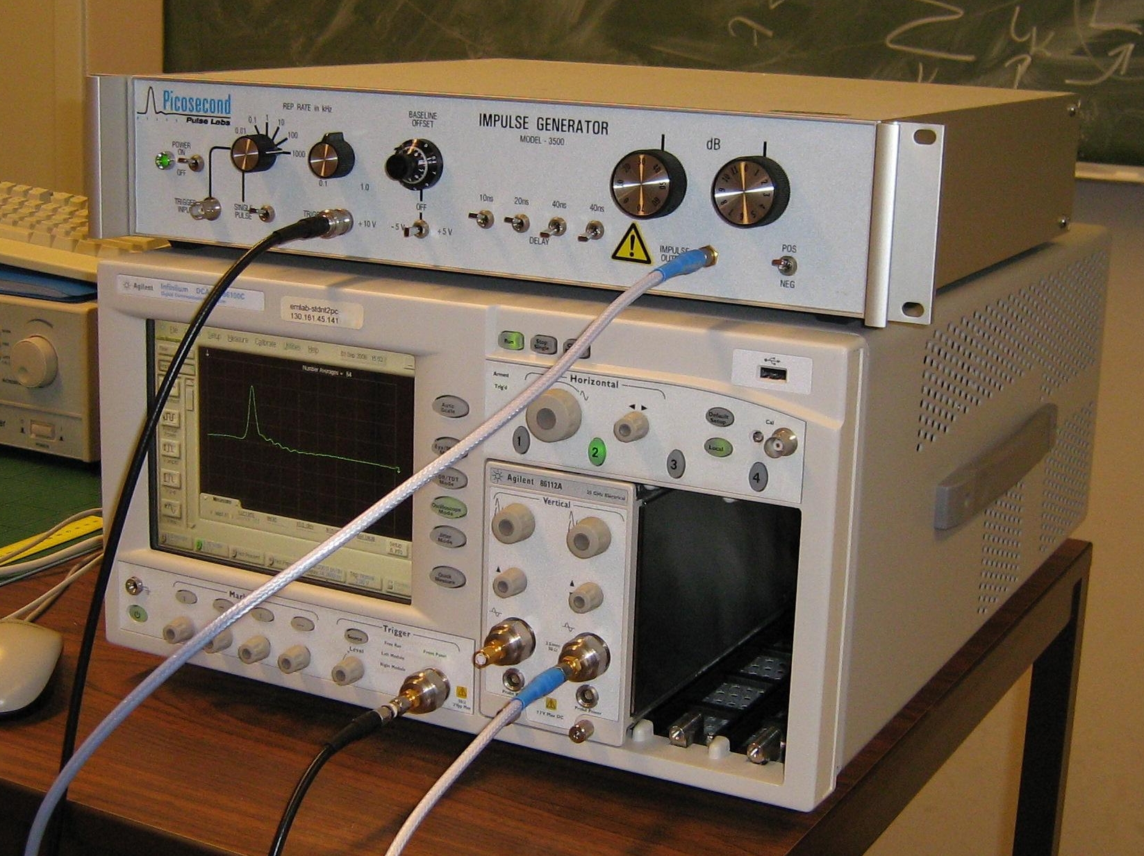
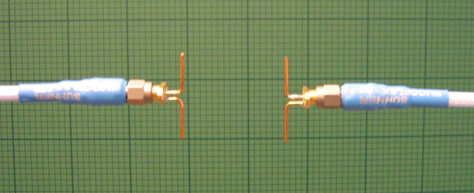
Figure 1: Equipment used to measure the velocity of electromagnetic waves. Upper photo: impulse generator on top of a sampling oscilloscope. Lower photo: dipole antennas attached to broadband co-axial cables (dipoles are less than 3 cm long).

The author’s plan was to follow the following simple routine:

1. receive the same signal at two locations, one further away from the source than the other;

2. choose some characteristic feature of the received waveform, say, the first maximum;

3. measure the absolute arrival times of this feature at two locations;

4. divide the difference between the distances of the two receivers to the source by the difference between the corresponding arrival times.

The result of the last calculation must be equal to the speed of light in vacuum. The required picosecond temporal resolution is routinely achieved nowadays with an impulse generator producing almost identical impulses and trigger signals at a precisely controlled repetition rate. The remaining jitter is taken care of by averaging over many realization of the pulse. The absolute arrival times here are measured in the same (stationary) reference frame, and in fact using the same well-calibrated device – the sampling oscilloscope – with time-zero set at a fixed time-interval with respect to the trigger.

Let the relative (radial) distance between the receiver locations be 12 cm. Then, the relative difference in arrival times must be

$$\Delta t=\frac{0.12\;{\rm m}}{299792458\;{\rm m/s}}=0.40028\;{\rm ns}.$$ (5)

In Fig. 2 and Fig. 3 we see the results of actual measurements. The first measurement is performed near the source: receivers at 9 cm and 21 cm. In the second measurement the receivers are at 30 cm and 42 cm. Thus, both figures correspond to the 12 cm relative spatial separation of the receivers. As we have some freedom in choosing a waveform feature to mark the arrival times, we compare the results obtained using the first and the third maximum of the waveform.

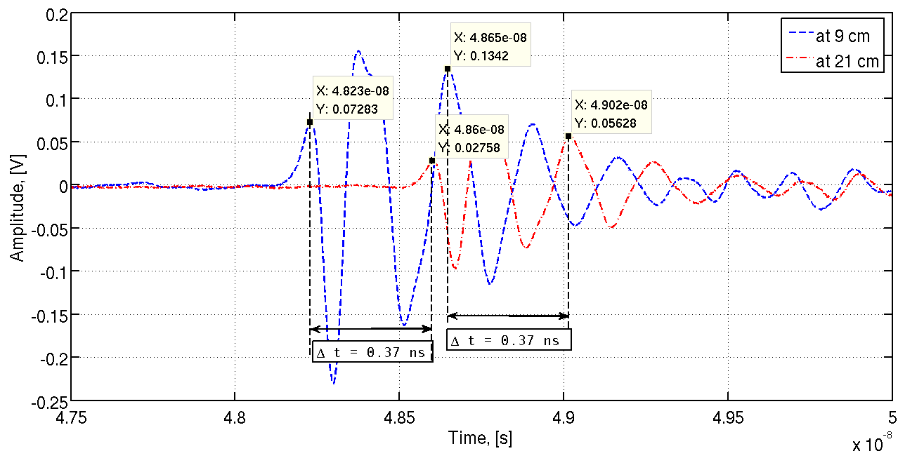
Figure 2: Superluminal propagation as seen in two-point near-field measurements. These signals were measured at 9 and 21 cm from the source (12 cm spatial separation). The arrival-time difference is too small: $\Delta t=0.37$ ns.

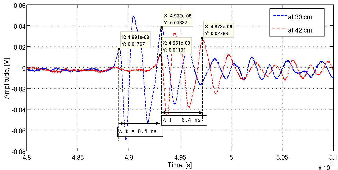
Figure 3: Further away from the source propagation happens at the speed of light. These signals were measured at 30 and 42 cm from the source (same 12 cm spatial separation as in Fig. 2). The arrival-time difference is now as expected: $\Delta t=0.4$ ns.

The data tips shown in the figures contain the absolute time values in seconds ($X$-axis data) at the extrema together with the corresponding voltage values (irrelevant to us here). The absolute time values are used to calculate $\Delta t$.

To the surprise and confusion of students only the second set of measurements, for the receivers at 30 cm and 42 cm, gives the correct answer, i.e., $\Delta t=0.4$ ns. The relative difference in the arrival times closer to the source is consistently smaller, e.g. $\Delta t=0.37$ ns in Fig. 2, showing superluminal propagation!

Nothing can travel faster than light. Hence, either the measurements are completely wrong or the maxima of a waveform cannot be regarded as true physical entities, i.e., cannot be the carriers of information. On the other hand, such waveform features are routinely used to transmit data and deduce distances to objects (travel time tomography), see e.g. Valle et al (1999) and Skolnik (2001). Could it be that the two-point measurement procedure does not determine the velocity? Yet, this procedure represents the very definition of velocity. It turns out that the resolution of this puzzle can be found in the classical radiation formula relating the current in the source and the field at the receiver.

3 Causality, compatibility, continuity, and gauge fixing.

The Maxwell equations in vacuum

$$\begin{split}-\nabla\times\mathbf{H}(\mathbf{x},t)+\varepsilon_{0}\partial_{t}\mathbf{E}(\mathbf{x},t)&=-\mathbf{J}(\mathbf{x},t),\\ \nabla\times\mathbf{E}(\mathbf{x},t)+\mu_{0}\partial_{t}\mathbf{H}(\mathbf{x},t)&=\mathbf{0},\end{split}$$ (6)

give the local relation between the source, current density $\mathbf{J}$, and the fields, electric and magnetic field strengths $\mathbf{E}$ and $\mathbf{H}$. To relate the source at one location to the fields at another one has to solve the Maxwell equations, i.e., derive the radiation formula. Explicit solutions of this kind can be obtained only in some elementary cases, such as the homogeneous background medium we consider here. We are particularly interested in the way the speed of light $c=1/\sqrt{\varepsilon_{0}\mu_{0}}$ enters the radiation formula, how exactly it reflects the causality of the radiation process, and whether this causality extends to such obvious and practically important features of the waveform as its extrema.

Causality is an assumption that the fields $\mathbf{E}$ and $\mathbf{H}$ are caused by the current $\mathbf{J}$. We must ensure therefore that the left- and right-hand sides of the Maxwell equations are compatible, i.e., all sources are accounted for by the current density $\mathbf{J}$. To see what it really means let us reduce the Maxwell’s system of two first-order equations to the second-order vector wave equation:

$$\nabla\times\nabla\times\mathbf{E}(\mathbf{x},t)+\frac{1}{c^{2}}\partial_{t}^{2}\mathbf{E}(\mathbf{x},t)=-\mu_{0}\partial_{t}\mathbf{J}(\mathbf{x},t).$$ (7)

From the first of the Maxwell equations we derive the following compatibility relation:

$$\varepsilon_{0}\partial_{t}\nabla\cdot\mathbf{E}(\mathbf{x},t)=-\nabla\cdot\mathbf{J}(\mathbf{x},t).$$ (8)

Temporal causality is often introduced as an assumption that no field existed before the initial switch-on moment $t_{0}$. Hence, we can re-write the local (in time) relation (8) as a time-integrated formula

$$\nabla\cdot\mathbf{E}(\mathbf{x},t)=-\frac{1}{\varepsilon_{0}}\nabla\cdot\int_{t_{0}}^{t}\mathbf{J}(\mathbf{x},t^{\prime})\,{\rm d}t^{\prime}.$$ (9)

For an “adiabatic” source one should take $t_{0}\rightarrow-\infty$. Now, using this expression and identity $\nabla\times\nabla\times\mathbf{E}=\nabla\nabla\cdot\mathbf{E}-\Delta\mathbf{E}$ we reduce the vector wave equation (7) to the usual scalar wave equation

$$\Delta\mathbf{E}(\mathbf{x},t)-\frac{1}{c^{2}}\partial_{t}^{2}\mathbf{E}(\mathbf{x},t)=-\frac{1}{\varepsilon_{0}}\nabla\nabla\cdot\int_{t_{0}}^{t}\mathbf{J}(\mathbf{x},t^{\prime})\,{\rm d}t^{\prime}+\mu_{0}\partial_{t}\mathbf{J}(\mathbf{x},t),$$ (10)

where the left-hand side is in its standard form (1) and the source term is explicitly identified.

The compatibility relation (9), is not only a key step in transforming the Maxwell equations into the wave equation (10), but has a connection to gauge fixing as well. To see this recall that the solution of Eq. (10) can be expressed via the solution of the same equation with a simpler right-hand side. Indeed, transform Eq. (10) into the $(\mathbf{k},s)$-domain using the three-dimensional spatial Fourier and the one-dimensional temporal Laplace transforms:

$$-(|\mathbf{k}|^{2}+\frac{s^{2}}{c^{2}})\tilde{\mathbf{E}}(\mathbf{k},s)=\frac{1}{s\varepsilon_{0}}\mathbf{k}\mathbf{k}\cdot\tilde{\mathbf{J}}(\mathbf{k},s)+s\mu_{0}\tilde{\mathbf{J}}(\mathbf{k},s).$$ (11)

Solution of this algebraic equation can be written as

$$\tilde{\mathbf{E}}(\mathbf{k},s)=-\frac{c^{2}}{s}\mathbf{k}\mathbf{k}\cdot\tilde{\mathbf{A}}(\mathbf{k},s)-s\tilde{\mathbf{A}}(\mathbf{k},s),$$ (12)

where

$$\tilde{\mathbf{A}}(\mathbf{k},s)=\frac{\mu_{0}}{|\mathbf{k}|^{2}+s^{2}/c^{2}}\tilde{\mathbf{J}}(\mathbf{k},s),$$ (13)

and it is easy to deduce by inverse transformations that the new quantity $\mathbf{A}(\mathbf{x},t)$ satisfies

$$\Delta\mathbf{A}(\mathbf{x},t)-\frac{1}{c^{2}}\partial_{t}^{2}\mathbf{A}(\mathbf{x},t)=-\mu_{0}\mathbf{J}(\mathbf{x},t).$$ (14)

The inverse transformation of Eq. (12) shows that there is a (spatially) local relation between the solutions of Eq. (10) and Eq. (14), namely,

$$\mathbf{E}(\mathbf{x},t)=c^{2}\nabla\nabla\cdot\int_{t_{0}}^{t}\mathbf{A}(\mathbf{x},t^{\prime})\,{\rm d}t^{\prime}-\partial_{t}\mathbf{A}(\mathbf{x},t).$$ (15)

On the other hand we know that a similar local relation exists between the fields and the vector and scalar potentials, i.e.,

$$\mathbf{E}(\mathbf{x},t)=-\nabla\phi(\mathbf{x},t)-\partial_{t}\mathbf{A}(\mathbf{x},t).$$ (16)

We see that the two expressions, (15) and (16), are identical, if we employ the Lorenz gauge

$$\nabla\cdot\mathbf{A}(\mathbf{x},t)+\frac{1}{c^{2}}\partial_{t}\phi(\mathbf{x},t)=0,$$ (17)

in the following time-integrated form:

$$c^{2}\nabla\cdot\int_{t_{0}}^{t}\mathbf{A}(\mathbf{x},t^{\prime})\,{\rm d}t^{\prime}=-\phi(\mathbf{x},t).$$ (18)

The scalar potential, in general, also obeys a wave equation

$$\Delta\phi(\mathbf{x},t)-\frac{1}{c^{2}}\partial_{t}^{2}\phi(\mathbf{x},t)=-\frac{1}{\varepsilon_{0}}\rho(\mathbf{x},t),$$ (19)

which can be written as

$$\Delta\phi(\mathbf{x},t)-\frac{1}{c^{2}}\partial_{t}^{2}\phi(\mathbf{x},t)=\frac{1}{\varepsilon_{0}}\nabla\cdot\int_{t_{0}}^{t}\mathbf{J}(\mathbf{x},t^{\prime})\,{\rm d}t^{\prime},$$ (20)

if we use the following time-integrated form of the continuity equation:

$$\nabla\cdot\int_{t_{0}}^{t}\mathbf{J}(\mathbf{x},t^{\prime})\,{\rm d}t^{\prime}=-\rho(\mathbf{x},t).$$ (21)

Thus, employing the compatibility relation (9) to derive the wave equation and the Lorenz gauge fixing (18) required for the unique representation of fields via potentials are two completely equivalent procedures. Moreover, we have also established that this amounts to (follows from) relating the sources of the scalar and vector potentials via the integrated continuity equation (21). The underlying mathematical assumption here is that the current density $\mathbf{J}$ accounts for all the sources of the electromagnetic field. Hence, Eq. (21) describes all possible variations of the charge density $\rho$. From the physical point of view, we assume that any eventual “bare” charge can only be created by some explicit dynamical process which disrupts the initial electrical neutrality of the substance (e.g. chemical reaction). Therefore, a current – motion of charges – precedes and causes the accumulation of charge. This is an often neglected and more subtle part of the general causality assumption behind the radiation formula. It treats static field as a stationary long-time limit of an initially transient electromagnetic field. The very existence of this limit and therefore static fields as such is thus an open problem in this formulation.

4 Time-domain radiation formula

A detailed derivation of the radiation formula presented below can be found in De Hoop (1995). It proceeds by computing the inverse Fourier transform of the $(\mathbf{k},s)$-domain solution (12). We arrive at

$$\hat{\mathbf{E}}(\mathbf{x},s)=\nabla\nabla\cdot\frac{c^{2}}{s}\hat{\mathbf{A}}(\mathbf{x},s)-s\hat{\mathbf{A}}(\mathbf{x},s),$$ (22)

with

$$\hat{\mathbf{A}}(\mathbf{x},s)=\mu_{0}\int_{\mathbf{x}^{\prime}\in{\mathbb{R}}^{3}}g(\mathbf{x}-\mathbf{x}^{\prime},s)\hat{\mathbf{J}}(\mathbf{x}^{\prime},s)\,{\rm d}\mathbf{x}^{\prime},$$ (23)

where the scalar Green’s function is

$$g(\mathbf{x},s)=\frac{e^{-(s/c)|\mathbf{x}|}}{4\pi|\mathbf{x}|}.$$ (24)

At this stage it is convenient to carry out the spatial differentiations in the first term on the right in Eq. (22). The resulting formula is

$$\begin{split}\hat{\mathbf{E}}(\mathbf{x},s)&=\int_{\mathbf{x}^{\prime}\in{\mathbb{R}}^{3}}\frac{e^{-(s/c)|\mathbf{x}-\mathbf{x}^{\prime}|}}{4\pi|\mathbf{x}-\mathbf{x}^{\prime}|^{3}}\left[3{\mathbb{Q}}-{\mathbb{I}}\right]\frac{1}{s\varepsilon_{0}}\hat{\mathbf{J}}(\mathbf{x}^{\prime},s)\,{\rm d}\mathbf{x}^{\prime}\\ &+\int_{\mathbf{x}^{\prime}\in{\mathbb{R}}^{3}}\frac{e^{-(s/c)|\mathbf{x}-\mathbf{x}^{\prime}|}}{4\pi|\mathbf{x}-\mathbf{x}^{\prime}|^{2}}\left[3{\mathbb{Q}}-{\mathbb{I}}\right]\frac{1}{\varepsilon_{0}c}\hat{\mathbf{J}}(\mathbf{x}^{\prime},s)\,{\rm d}\mathbf{x}^{\prime}\\ &+\int_{\mathbf{x}^{\prime}\in{\mathbb{R}}^{3}}\frac{e^{-(s/c)|\mathbf{x}-\mathbf{x}^{\prime}|}}{4\pi|\mathbf{x}-\mathbf{x}^{\prime}|}\left[{\mathbb{Q}}-{\mathbb{I}}\right]\frac{s}{\varepsilon_{0}c^{2}}\hat{\mathbf{J}}(\mathbf{x}^{\prime},s)\,{\rm d}\mathbf{x}^{\prime}.\end{split}$$ (25)

The three terms above are called near-, intermediate-, and far-field contributions in accordance with their spatial decay factors. The tensors act as

$${\mathbb{Q}}\mathbf{J}(\mathbf{x}^{\prime}) =\frac{(\mathbf{x}-\mathbf{x}^{\prime})}{|\mathbf{x}-\mathbf{x}^{\prime}|}\left(\frac{(\mathbf{x}-\mathbf{x}^{\prime})}{|\mathbf{x}-\mathbf{x}^{\prime}|}\cdot\mathbf{J}(\mathbf{x}^{\prime})\right),$$ (26)

$${\mathbb{I}}\mathbf{J}(\mathbf{x}^{\prime}) =\mathbf{J}(\mathbf{x}^{\prime}).$$ (27)

The magnetic field can be found from a similar formula

$$\begin{split}\hat{\mathbf{H}}(\mathbf{x},s)&=-\int_{\mathbf{x}^{\prime}\in{\mathbb{R}}^{3}}\frac{e^{-(s/c)|\mathbf{x}-\mathbf{x}^{\prime}|}}{4\pi|\mathbf{x}-\mathbf{x}^{\prime}|^{2}}\mathbf{\Theta}\times\hat{\mathbf{J}}(\mathbf{x}^{\prime},s)\,{\rm d}\mathbf{x}^{\prime}\\ &-\int_{\mathbf{x}^{\prime}\in{\mathbb{R}}^{3}}\frac{e^{-(s/c)|\mathbf{x}-\mathbf{x}^{\prime}|}}{4\pi|\mathbf{x}-\mathbf{x}^{\prime}|}\frac{s}{c}\mathbf{\Theta}\times\hat{\mathbf{J}}(\mathbf{x}^{\prime},s)\,{\rm d}\mathbf{x}^{\prime},\end{split}$$ (28)

where

$$\mathbf{\Theta}=\frac{\mathbf{x}-\mathbf{x}^{\prime}}{|\mathbf{x}-\mathbf{x}^{\prime}|}.$$ (29)

Finally, the inverse Laplace transform gives the explicit time-domain formulas

$$\begin{split}\mathbf{E}(\mathbf{x},t)&=\int_{\mathbf{x}^{\prime}\in{\mathbb{R}}^{3}}\frac{3{\mathbb{Q}}-{\mathbb{I}}}{4\pi|\mathbf{x}-\mathbf{x}^{\prime}|^{3}}\frac{1}{\varepsilon_{0}}\int_{t_{0}}^{t_{\rm R}}\mathbf{J}(\mathbf{x}^{\prime},t^{\prime})\,{\rm d}t^{\prime}\,{\rm d}\mathbf{x}^{\prime}\\ &+\int_{\mathbf{x}^{\prime}\in{\mathbb{R}}^{3}}\frac{3{\mathbb{Q}}-{\mathbb{I}}}{4\pi|\mathbf{x}-\mathbf{x}^{\prime}|^{2}}\frac{1}{\varepsilon_{0}c}\mathbf{J}(\mathbf{x}^{\prime},t_{\rm R})\,{\rm d}\mathbf{x}^{\prime}\\ &+\int_{\mathbf{x}^{\prime}\in{\mathbb{R}}^{3}}\frac{{\mathbb{Q}}-{\mathbb{I}}}{4\pi|\mathbf{x}-\mathbf{x}^{\prime}|}\frac{1}{\varepsilon_{0}c^{2}}\partial_{t}\mathbf{J}(\mathbf{x}^{\prime},t_{\rm R})\,{\rm d}\mathbf{x}^{\prime}\end{split}$$ (30)

and

$$\begin{split}\mathbf{H}(\mathbf{x},t)&=-\int_{\mathbf{x}^{\prime}\in{\mathbb{R}}^{3}}\frac{1}{4\pi|\mathbf{x}-\mathbf{x}^{\prime}|^{2}}\mathbf{\Theta}\times\mathbf{J}(\mathbf{x}^{\prime},t_{\rm R})\,{\rm d}\mathbf{x}^{\prime}\\ &-\int_{\mathbf{x}^{\prime}\in{\mathbb{R}}^{3}}\frac{1}{4\pi|\mathbf{x}-\mathbf{x}^{\prime}|}\mathbf{\Theta}\times\frac{1}{c}\partial_{t}\mathbf{J}(\mathbf{x}^{\prime},t_{\rm R}),\,{\rm d}\mathbf{x}^{\prime}\end{split}$$ (31)

where for the first time we meet the retarded time

$$t_{\rm R}=t-\frac{|\mathbf{x}-\mathbf{x}^{\prime}|}{c},$$ (32)

which is an analogue of the $\pm ct$ shift of the d’Alembert solution (4). The spatial integration in (30) will in practice be limited to a finite domain $D_{\rm s}$ occupied by the source.

5 Explanation of near-field superluminal velocities

With the radiation formula (30) at hand we can start analyzing the shape of the waveforms received at some distance from the source. A waveform measured by the dipole antenna of the type shown in Fig. 1 gives the time-evolution of a single component of the electric field strength determined by the orientation of the dipole and modified by the the antenna-cable-oscilloscope receiving tract. The latter modification, however, is the same for all receiver locations, i.e., does not depend on the distance from the source. Only in the close proximity of the source the expected small multiple reflections between the two antennas may slightly modify the tail of the waveform with respect to what is predicted by Eq. (30).

A simplified formula for small source and receiver dipoles, parallel to each other and located in a plane orthogonal to their orientation (as in Fig. 1) is

$$V(\mathbf{x},t)\sim-\frac{1}{4\pi\varepsilon_{0}R^{3}}\int_{t_{0}}^{t_{\rm R}}I(t^{\prime})\,{\rm d}t^{\prime}-\frac{1}{4\pi\varepsilon_{0}cR^{2}}I(t_{\rm R})-\frac{1}{4\pi\varepsilon_{0}c^{2}R}\partial_{t}I(t_{\rm R}),$$ (33)

where $R$ is the distance between the dipoles, $t_{\rm R}=t-R/c$, $V$ is the measured waveform, and $I$ is the signal (current) in the source antenna.

Obviously, the received waveform is a function not only of the signal $I$ at an earlier time, but also of its time-derivative and time-integral. Figure 4 shows the three functions in question

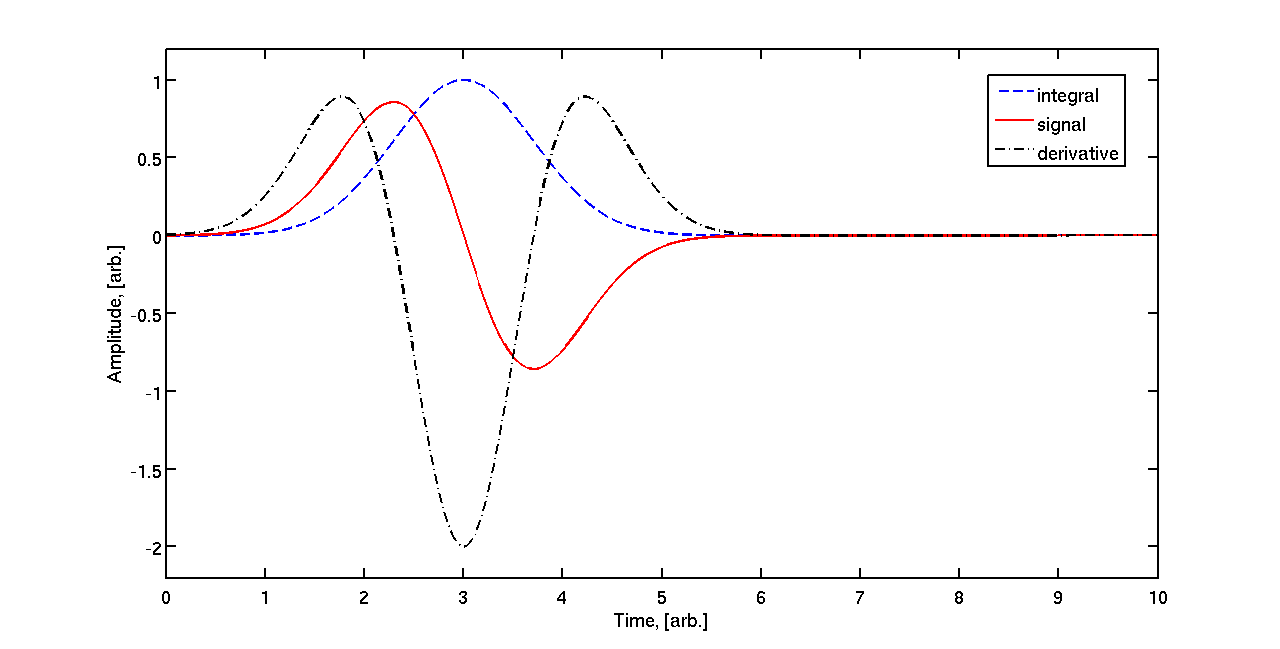
Figure 4: Back-in-time shifting of extrema. Depicted are the signal, its cumulative time-integral, and derivative. The first extremum of the integral is further (later) in time, whereas the first extremum of the derivative is earlier in time than the first extremum of the original signal.

for the current of the form

$$I(t)=-2\alpha(t-t_{\rm c})e^{-\alpha(t-t_{\rm c})^{2}},$$ (34)

whose integral and derivative can be computed analytically. As can be seen from Fig. 4 the extrema of the three functions are time-shifted with respect to each other. In the present case we can talk about the first extremum only, since the integral does not have a second one. With respect to this first extremum we notice that the integral has it later, and the derivative has it earlier in time than the function itself. This is a purely mathematical phenomenon and it will be observed with any function.

The received waveform is a weighted sum of these three functions. The weight coefficients are the functions of distance $R$ between the source and the receiver, where the term with $R^{-3}$ will be dominant close to the source (near-field zone), and the term with $R^{-1}$ is dominant for large $R$ (far-field zone). This means that in the near-field zone the received waveform will look almost like the integral, and in the far-field zone it will look almost like the derivative of the current.

The two-point procedure described in Section 2 deduces the velocity of the electromagnetic pulse from the waveform measured at two locations where one is further away from the source. Thus, according to Eq. (34) the values of the weighting factors will be different for these two locations. Not only the waveform will be smaller in amplitude for the more distant of the two locations, but the relative weight of the three contributions will change as well. In general the relative weight of the last term increases, whereas the relative weight of the first term decreases with distance. Hence, we may expect the shape of the waveform to gradually change from the one dominated by the time-integrated signal to the one dominated by the time-derivative of the signal. As can be seen from Fig. 4 this means a shift of an extremum towards earlier times. Such backward in time “motion” will be superimposed on the normal time-delay which shifts the received waveform to the right along the time axis as one moves further away from the source.

The latter observation explains our failure to measure the speed of light in Section 2. Indeed, the first measurement location in Fig. 2 is close enough to the source for the influence of the near- and intermediate-field terms to be significant. Therefore, the overall waveform is somewhat shifted to the right along the time-axis relative to the time-delayed derivative of the original signal, which is dominant at larger distances. At the second location the influence of the near- and intermediate-field terms is smaller and so is the relative shift. Let us express the arrival times of the measured extrema at two locations as

$$\begin{split}t_{\rm arr}(R_{1})&=t_{0}+\frac{R_{1}}{c}+\Delta t(R_{1}),\\ t_{\rm arr}(R_{2})&=t_{0}+\frac{R_{2}}{c}+\Delta t(R_{2}),\end{split}$$ (35)

where $\Delta t(R)$ is the relative shift due to the near- and intermediate-field terms. We give it a positive sign to emphasize that the relative time-shift is happening towards later (positive) times on top of the normal propagation induced positive time-delay $R/c$.

The speed of light was deduced in Section 2 from the following simple two-point calculation:

$$c_{\rm exp}=\frac{R_{2}-R_{1}}{t_{\rm arr}(R_{2})-t_{\rm arr}(R_{1})},$$ (36)

applied to the extrema of the measured waveform. It is easy to see, that without the additional relative time-shifts $\Delta t$, substitution of (35) would have given us the exact speed of light. Now, however, the denominator in (36) is

$$t_{\rm arr}(R_{2})-t_{\rm arr}(R_{1})=\frac{R_{2}-R_{1}}{c}+\Delta t(R_{2})-\Delta t(R_{1}).$$ (37)

Since the relative time-shift $\Delta t(R)$ is diminishing with distance, we have in general

$$\Delta t(R_{2})-\Delta t(R_{1})<0,\;\;\;R_{2}>R_{1},$$ (38)

Thus, the measured time difference is always smaller then the expected one. If this time difference is positive we get

$$c_{\rm exp}>c,$$ (39)

i.e., the measured speed is superluminal – exactly as we have observed.

That this superluminal behavior is not visible in Fig. 3, and in the majority of experiments with light, can also be explained. The near- and intermediate-field terms, which cause the additional time shift, decay not only relatively with respect to the far-field term, but also absolutely, i.e., their influence is practically not measurable in the far field. The far-field zone is a notion relative to the wavelength. Usually, the far-field zone starts beyond a few tens of wavelengths, i.e., is very close to the source for the visual light.

The measured speed reflects two competing phenomena – outward propagation and the diminishing additional positive time shift. In the far-field zone the first of these phenomena gradually takes over, and we may expect the local two-point measurement procedure to yield values of speed progressively approaching the speed of light from above, as if the pulse was decelerating. In the near-field zone, however, the additional time shift is large enough to be detectable. We saw how it yields superluminal values for the pulse speed. Obviously, we need to let go of the idea of a constant speed and consider a more general concept of a local velocity which is a function of distance from the source. For example, we could introduce a local velocity as a limit of the two-point measurement procedure in the neighborhood of some location $R$ as

$$v_{\rm loc}(R)=\lim\limits_{\epsilon\rightarrow 0}\frac{\epsilon}{t^{\rm ex}(R+\epsilon)-t^{\rm ex}(R)},$$ (40)

where $t^{\rm ex}(R)$ is the time of the waveform extremum measured at location $R$. This definition, however, is hard to apply as we do not know the above extrema times explicitly.

6 Locally negative velocities

As was mentioned above superluminal pulse propagation is observed, if the measured time difference in the two-point procedure is smaller than the expected $R/c$, but remains positive. If this difference is negative, then the measured velocity would also become negative. Are such negative velocities possible, and what does it mean? The answer can be obtained with the formulas and understanding we have acquired in the previous section. Indeed, a negative velocity could be measured in a two-point procedure, if the anomalous positive time-shift we discussed was disappearing faster with $R$ than the normal growth of the positive time-shift due to propagation, i.e.,

$$\frac{R_{2}-R_{1}}{c}<\Delta t(R_{1})-\Delta t(R_{2}).$$ (41)

Recently an experiment was reported by the author, Budko (2009). It showed that this effect is indeed present and can be observed with the setup which we used above to demonstrate the superluminal pulse velocities. Very close to the source the waveform shows a small but detectable movement towards earlier times (to the left on the scope screen) as we move the receiver away from the source in small steps. Figure 5 shows the results of this experiment.

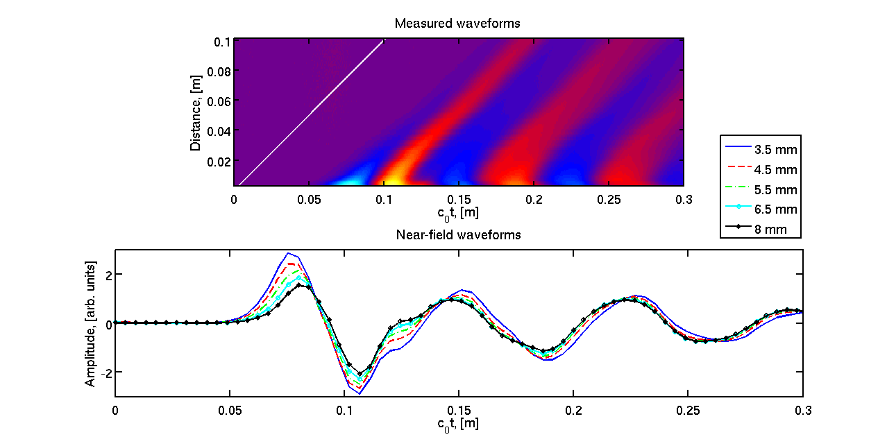
Figure 5: Experimental demonstration of local negative pulse velocity in the near-field of a small dipole antenna. Upper image shows the space-time dynamics of the signal. Close to the source (bottom of the image) the wave makes a small bend to the left along the time axis – negative velocity region. Further from the source the wave dynamics approaches the light-cone behavior (white line). Lower plot shows the wave dynamics in the near-field zone. While the wavefront and the first slope shift towards later times (positive velocity), the extrema and the whole inner part of the waveform shift to the left (negative velocity).

The measurements had to be carried out very close to the source. For the $75$-ps pulse that was used in the experiment the negative velocity region is within $10$ mm distance from the source. The extent of the negative-velocity region was initially predicted by a simulation similar to the one considered in the next section. The actual measurements also contain multiple reflections between the source and receiver dipoles. These reflections show as a small bump in the slope of the waveform between $c_{0}t=0.1$ and $c_{0}t=0.15$ m. This was verified by inserting a larger metallic scatterer in the plain of the source and observing an increase of the said bump as well as the appearance of multiples further down the tail of the waveform. Apart from that the leftward shift of the inner part of the waveform is clearly visible. The upper image in Fig. 5 is a rotated version of a typical light-cone diagram from special relativity. In fact, the white line indicates the way the light cone is supposed to be. If the light was indeed following its “cone”, then the colored stripes in the image should all follow that white line. This happens only further away from the source. Whereas in the bottom of the image there is an obvious near-field distortion – a leftward bend corresponding to the negative velocity of propagation.

Such behavior is very counterintuitive and may even seem anti-causal. Indeed, it looks like the signal reaches a more distant observer faster than a closer one. Although information may be and often is encoded in extrema of a waveform the speed at which it reaches the observer is hard to define. We notice from the experimental data in Figure 5 that the front of the wave travels with a positive velocity. Moreover, for a source current with a sharp temporal boundary $I(t)=0$, $t\leq t_{0}$ we can prove analytically that the wavefront always travels outwards at the speed of light, since near- and intermediate-field terms are exactly zero for $t=t_{\rm R}$ in that case. For the same reason the end of the waveform would also travel outwards and at the speed of light. Thus, the beginning and the end of an information carrying wave-packet would arrive at two observes in a proper relativistically consistent temporal order, i.e., later for the more distant observer. However, due to the anomalous temporal shift of extrema the more distant observer may actually receive the information sooner than the closer one. Of course, we are talking about the near-field zone and two very close observers, but nevertheless. Explanation seems to be in the fact that the two observes are causally related to the source of the field, but not to each other. The situation becomes less paradoxical if we put it this way: it is not that the more distant observer gets the information faster than normal. No, the beginning of the information packet arrives at the speed of light. It is that the closer of the two observers receives the same information slower than normal, due to the additional positive time-shift of the waveform in the near-field zone. The same explanation helps to comprehend the superluminal impulse velocities observed earlier.

7 Negative power flow

At the moment the strange velocities we observe in the near-field zone seem to be tightly linked to the two-point measurement procedure and our choice of extrema as the reference points. To show that the two-point procedure is not really essential here let us look at the power flow in the near-field zone. An analysis along the following lines, although focused on the Hertzian dipole with an initial static field, can be found in Schantz (2001). The instanteneous power density flowing through location $\mathbf{x}$ at time $t$ is given by the Poynting vector

$$\mathbf{S}(\mathbf{x},t)=\mathbf{E}(\mathbf{x},t)\times\mathbf{H}(\mathbf{x},t).$$ (42)

In our particular experimental arrangement with a small source the current density can be approximated by

$$\mathbf{J}(\mathbf{x},t)=\mathbf{d}I(t)\delta(\mathbf{x}-\mathbf{x}_{\rm s}),$$ (43)

where $\mathbf{d}$ is a unit vector in the direction of the current. For the geometry depicted in Fig. 1 we have

$$\mathbf{S}(R,t)=P(R,t)\mathbf{\Theta},$$ (44)

where the unit vector $\mathbf{\Theta}$ points away from the source towards the receiver and the power density amplitude is

$$\begin{split}P(R,t)&=\left[\frac{1}{4\pi\varepsilon_{0}R^{3}}\int_{t_{0}}^{t_{\rm R}}I(t^{\prime})\,{\rm d}t^{\prime}+\frac{1}{4\pi\varepsilon_{0}cR^{2}}I(t_{\rm R})+\frac{1}{4\pi\varepsilon_{0}c^{2}R}\partial_{t}I(t_{\rm R})\right]\times\\ &\left[\frac{1}{4\pi R^{2}}I(t_{\rm R})+\frac{1}{4\pi cR}\partial_{t}I(t_{\rm R})\right]\\ &=\frac{1}{(4\pi)^{2}\varepsilon_{0}R^{5}}I(t_{\rm R})\int_{t_{0}}^{t_{\rm R}}I(t^{\prime})\,{\rm d}t^{\prime}+\frac{1}{(4\pi)^{2}\varepsilon_{0}cR^{3}}\partial_{t}I(t_{\rm R})\int_{t_{0}}^{t_{\rm R}}I(t^{\prime})\,{\rm d}t^{\prime}+\\ &\left[\frac{1}{4\pi\varepsilon_{0}^{1/2}c^{1/2}R^{2}}I(t_{\rm R})+\frac{1}{4\pi\varepsilon_{0}^{1/2}c^{3/2}R}\partial_{t}I(t_{\rm R})\right]^{2}.\end{split}$$ (45)

While the last term is undoubtedly positive at all times, the remaining two terms may, in principle, become negative due to the mixed products of the current, its derivative, and integral, which as we know can all have different signs at the same time – see Fig. 4. If a negative power flow can be detected, the phenomenon would again be confined to the near-field zone, as the dominant far-field term is positive.

Let us consider another current pulse with analytically known derivative and integral. This time, however, we shall look at a pulse called monocycle with well-defined beginning and end:

$$\begin{split}I(t)=\left\{\begin{array}[]{l}\sin(\omega t),\;\;\;t\in[t_{0},t_{0}+2\pi/\omega],\\ 0,\;\;\;t\notin[t_{0},t_{0}+2\pi/\omega],\end{array}\right.\end{split}$$ (46)

where $\omega$ is the carrier frequency. The derivative and integral of this signal within the time interval $[t_{0},t_{0}+2\pi/\omega]$ are:

$$\begin{split}\partial_{t}I(t)&=\omega\cos(\omega t),\\ \int_{t_{0}}^{t}I(t^{\prime})\,{\rm d}t^{\prime}&=\frac{1}{\omega}\left[\cos(\omega t_{0})-\cos(\omega t)\right],\end{split}$$ (47)

and are zero outside the said interval. The normalized versions of these functions are shown in the top plot of Fig. 6 for $\omega=8\pi\times 10^{9}$, i.e., for a $4$ GHz carrier frequency.

Figure 6: Top: mono-cycle source current, its integral, and derivative (normalized). Bottom: Simulated electric field at various distances from the source (normalized). Close to the source the received signal resembles the integral taken with a negative sign. Further it deforms into a shifted negative of the signal, and finally transforms into a negative of the derivative of the signal. The negative velocity phenomenon is obvious between $1$ mm and $15$ mm distances – waveform shifts leftwards.

The bottom plot of that figure shows the results of simulation of the electric field at three different distances from the source: $1$, $15$, and $50$ mm. We use Eq. (33) to simulate the waveforms. All pertaining deformations of the waveform are now clearly visible, as it resembles the integral of the signal in the near-field zone and gradually transforms into the derivative of the signal as we measure further away. We also see the negative velocity phenomenon as the inner part of the waveform at $15$ mm is clearly shifted to the left, instead of being shifted to the right of the waveform corresponding to $1$ mm distance. At the same time the wavefront and the end of the waveform do shift rightwards as predicted.

To understand, at least mathematically, the emergence of the negative power flow consider a very small distance $R$, such that the first terms in Eq. (45) are dominant. These terms contain mixed products of the current, its integral, and derivative. For the particular current given by Eq. (46)–(47) we see that these mixed products will be negative over a certain period of the time – see Fig. 8 (top). Although we do not prove it here rigorously for an arbitrary current, computer simulations and common sense indicate that the time-integrated power is positive at all distances, including the near-field zone – see Fig. 7. This, however, does not exclude the possibility of instantaneous power being negative for some time.

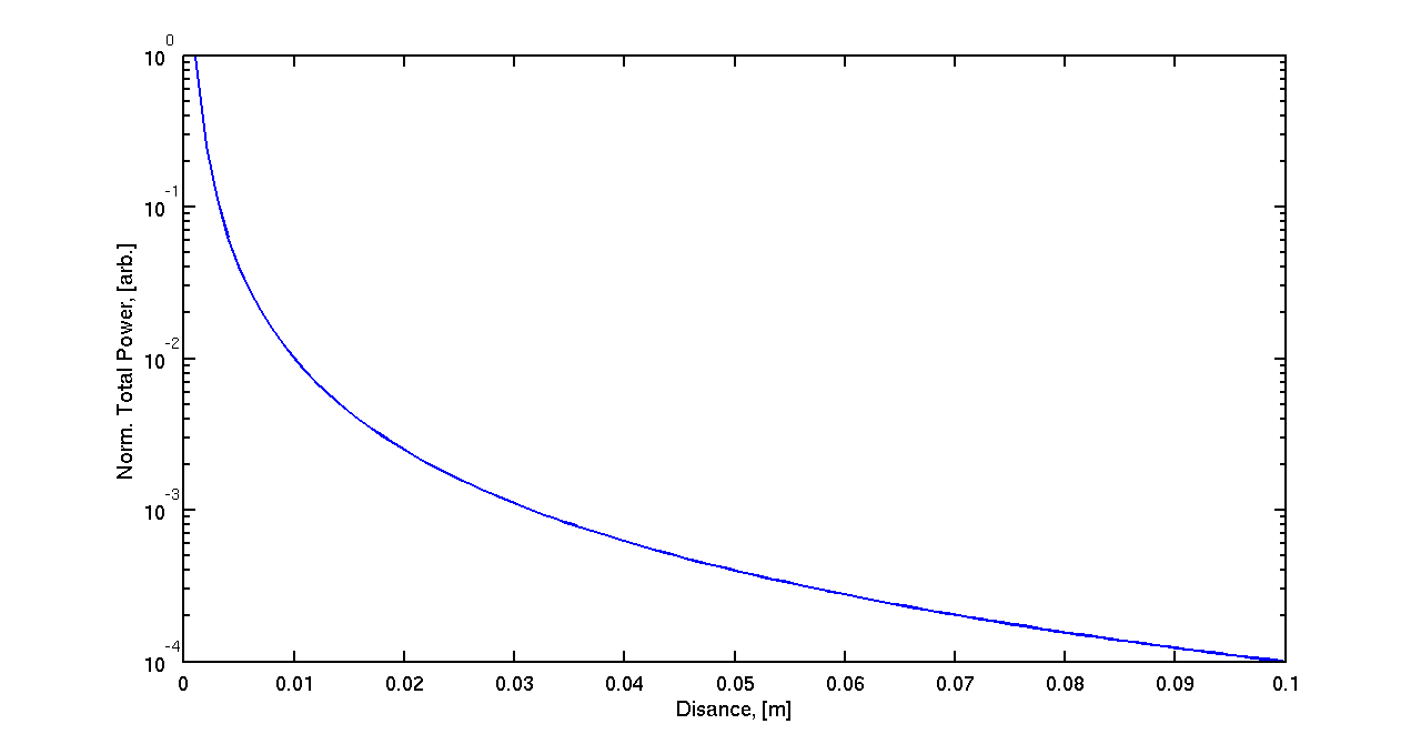
Figure 7: Normalized time-integrated power as a function of distance from the source. This quantity is positive everywhere.

In Figure 8 (bottom) we see the power $P(R,t)$ as a function of time

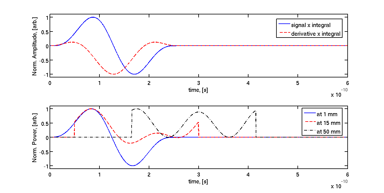
Figure 8: Top: normalized products of the signal and its integral, and derivative of the signal and signal’s integral corresponding to the source current shown in Fig. 6. Notice the presence of negative parts in both cases. Bottom: normalized instantaneous power flow at various distances from the source. In the near-field zone the power flow can become negative for some time. During that time power flows towards the source. Further from the source the power flow looks positive at all times (see, however, Fig. 9).

at three distances from the source. The negative power flow is clearly visible in this plot. As we move towards the far-field zone the power flow looks positive at all times. This, however, is not true as we shall see in the next Section.

Power flow tells us how much energy is coming from a certain direction in a unit of time. If a power flow is negative it means that the energy is decreasing with time, or that the power is flowing towards the source of radiation, instead of away from it. Since the Poynting vector is related to the density of the linear momentum of the electromagnetic field, we may expect the instantaneous pressure of light to change its direction over extremely short time intervals in the near-field zone. Not only the light will be pushing away from the source, as it is usually the case, but pulling towards the source as well. This may induce a very rapid mechanical oscillation on a neutral test particle – an opto-mechanical effect which might be of interest in nano-physics.

8 Energy velocity

We can formally relate the power flow and the energy density in our experimental setup via the following formula:

$$P(\mathbf{x},t)\mathbf{\Theta}=v_{\rm e}(\mathbf{x},t){\mathcal{E}}(\mathbf{x},t)\mathbf{\Theta},$$ (48)

where ${\mathcal{E}}$ is the local instantaneous energy of the electromagnetic field. From where the energy velocity along $\mathbf{\Theta}$ is expressed as

$$v_{\rm e}(\mathbf{x},t)=\frac{P(\mathbf{x},t)}{{\mathcal{E}}(\mathbf{x},t)}.$$ (49)

Simulations of the energy velocity for a transient Hertzian dipole were presented by Marcano & Diaz (2006). Since, as we saw above, the local power flow can be negative, while the field energy is always positive, the near-field zone results of Marcano & Diaz (2006) naturally contained locally negative energy velocities.

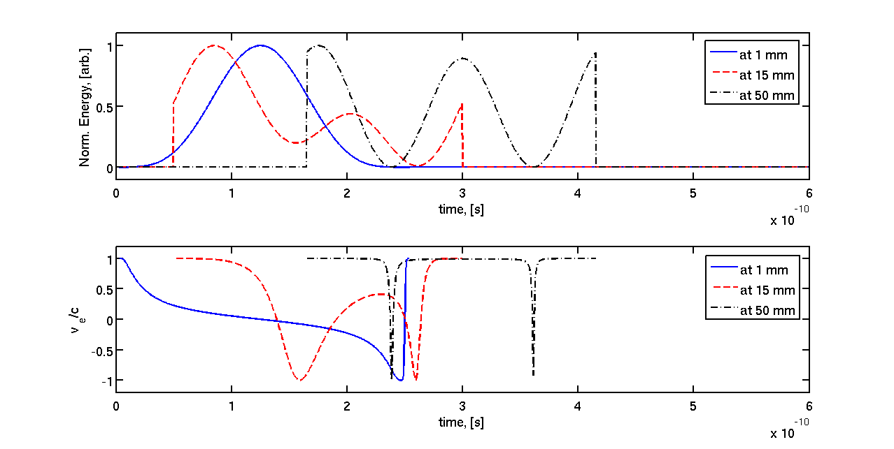
Figure 9: Top: normalized local instantaneous energy at various distances corresponding to the source current shown in Fig. 6. Bottom: Relative energy velocity, $v_{\rm e}/c$, at various distances from the source.

The power amplitude for our measurement configuration is given by Eq. (45), whereas the energy density at location $R$ as a function of time is

$$\begin{split}{\mathcal{E}}(R,t)&=\varepsilon_{0}\left[\frac{1}{4\pi\varepsilon_{0}R^{3}}\int_{t_{0}}^{t_{\rm R}}I(t^{\prime})\,{\rm d}t^{\prime}+\frac{1}{4\pi\varepsilon_{0}cR^{2}}I(t_{\rm R})+\frac{1}{4\pi\varepsilon_{0}c^{2}R}\partial_{t}I(t_{\rm R})\right]^{2}+\\ &\mu_{0}\left[\frac{1}{4\pi R^{2}}I(t_{\rm R})+\frac{1}{4\pi cR}\partial_{t}I(t_{\rm R})\right]^{2}.\end{split}$$ (50)

This function for the monocycle source current Eq. (46) and the corresponding instantaneous relative energy velocity $v_{\rm e}(R,t)/c$ are shown in Fig. 9. Similar to the waveform of the electric field, the waveform of the instantaneous energy deforms as one moves through the near-, intermediate-, and far-field zones. There is no doubt about the positivity of energy density at all locations and times due to the intrinsic mathematical form of expression Eq. (50). Thus, the negative values of the energy velocity visible in Fig. 9 (bottom) are caused by the locally negative power amplitude. It is obvious, that the energy velocity varies between $-c$ and $c$. It is also obvious that the energy velocities of the front and the end of the wave-packet are both exactly the speed of light, and that the deviations concern the inner part of the waveform only. We notice that the subluminal and negative velocities are mainly featured in the near-field zone and that the far-field energy waveform moves mostly at the speed of light. However, at the time instant where both energy and power tend to zero, the energy velocity makes a sharp swing to $-c$ and back even in the far-field zone. This shows that the power amplitude must be going slightly negative at the minima of the far-field waveform, something we could not previously detect in Fig. 8. Thus, although the local instantaneous energy velocity seems to be a very natural concept, and its magnitude is explicitly bounded by the speed of light, it also magnifies the effect of the first two terms in Eq. (45), so that it is felt even in the far-field zone, albeit for a vanishingly small time. Whether this swing in the power flow can be detected remains to be seen.

9 Conclusions

We have discussed a series of unusual transient effects in the electromagnetic radiation from a localized source. These effects demonstrate that the space-time evolution of the electromagnetic field is nothing like a simple outwards propagation of a spherical wave at the speed of light. In fact, the speed of light could only be assigned to the boundary between the field and the area free from it – the wavefront and the end of a wave-packet. The inner part of the wave-packet undergoes significant deformation in the course of propagation. This deformation leads, in particular, to superluminal and negative velocity results with the classical two-point velocity measurement procedure. We have uncovered that the source of this deformation is an anomalous time delay, which the waveform undergoes in the immediate vicinity of the source. It takes more time for, say, an extremum to build up close to the source than a little further away. Hence, paradoxically, it takes more time for the information to arrive at a closer observer than at an observer further away from the source. Yet, both transmission times are within what is allowed by the relativity theory. While this effect can be observed only very close to the source, the other related phenomenon can be measured in the intermediate-field zone as well.

The anomalous time delay rapidly decays with the distance from the source. Hence, the time-interval measured in the two-point procedure is usually smaller than what is expected from the propagation at the speed of light. This explains the observed superluminal results and shows the necessity of near-field corrections to the travel-time algorithms used in geophysics and radar imaging, such as those used in e.g. Valle et al (1999) and Skolnik (2001).

We have also considered the instantaneous power flow from a transient source. In the near-field zone power may flow towards the source for some time. Although, the time-integrated power flow stays positive, a positive instantaneous power flow followed by a negative flow during a significant interval of time will induce an oscillating linear momentum and an oscillating instantaneous light pressure.

Finally, we have analyzed the local instantaneous energy velocity which is conveniently bounded between $-c$ and $c$. Its waveforms show that the energy velocities of the wavefront and the end of a wave-packet are both exactly $c$, and that the subluminal and negative values during extended time intervals are the feature of the near-field zone only. At the same time the energy velocity reveals that the power flow can become negative for a short time even in the far-field zone. This happens when both the power flow and the energy are close to zero, and it remains to be seen whether this effect can be detected experimentally.

On a theoretical level all these unusual effects and their experimental confirmation show the correctness of the time-domain radiation formula (30)–(31). We have demonstrated how this formula follows from the Lorenz gauge-fixing between the classical scalar and vector potentials and eventually reduces to the continuity equation between the current and charge densities. These otherwise somewhat ad hoc procedures thus acquire additional physical significance.

References

- [1] Bajcsy, M., Zibrov, A. S. and Lukin, M. D. (2003) ‘Stationary pulses of light in an atomic medium’, Nature 426, pp. 638–641.
- [2] Bialynicki-Birula, I., Cirone, M. A., Dahl, J. P., Fedorov, M. and Schleich, W. P. (2002) ‘In- and Outbound Spreading of a Free-Particle s-Wave’, Phys. Rev. Lett. 89, 060404.
- [3] Budko, N. V. (2009) ‘Observation of Locally Negative Velocity of the Electromagnetic Field in Free Space’, Phys. Rev. Lett. 102, 020401.
- [4] Cirone, M. A., Dahl, J. P., Fedorov, M., Greenberger, D. and Schleich W. P. (2002) ‘Huygens’ principle, the free Schrödinger particle and the quantum anti-centrifugal force’, J. Phys. B 35, pp. 191–203.
- [5] De Hoop, A. T. (1995) Handbook of radiation and scattering of waves, Academic Press.
- [6] Diener, G. (1996) ‘Superluminal group velocities and information transfer’, Physics Letters A 223, pp. 327–331.
- [7] Giacomo, P. (1984), ‘News from BIPM’ Metrologia 20, pp. 25 – 30.
- [8] Heitmann, W. and Nimtz, G. (1994) ‘On causality proofs of superluminal barrier traversal of frequency band limited wave packets’ Physics Letters A 196, Issues 3-4,pp. 154–158.
- [9] Hau, L. V., Harris, S. E., Dutton, Z. and Behroozi, C. H. (1998) ‘Light speed reduction to 17 metres per second in an ultracold atomic gas’, Nature 397, pp. 594–598.
- [10] Landau, L. D. and Lifshitz, E. M. (1963) Electrodynamics of continuous media, Pergamon Press.
- [11] Marcano, D. and Diaz, M. (2006) ‘Energy Transport Velocity for Hertzian Dipole’, Proc. 2006 IEEE Antennas and Propagation Society International Symposium, pp. 2017–2020.
- [12] Mugnai, D., Ranfagni, A. and Ruggeri, R. (2000) ‘Observation of superluminal behavior in wave propagation’, Phys. Rev. Lett. 84, pp. 4830–4833. See also comments: Phys. Rev. Lett. 87, 059401-1, [2001]; Phys. Rev. Lett. 87, 059401-01, [2001].
- [13] Porras, M. A. (1999) ‘Nonsinusoidal few-cycle pulsed light beams in free space’, JOSA B 16, pp. 1468–1474.
- [14] Ranfagni, A., Fabeni, P., Pazzi, G. P. and Mugnai, D. (1993) ‘Anomalous pulse delay in microwave propagation: A plausible connection to the tunneling time’ Phys. Rev. E 48, pp. 1453–1460.
- [15] Ranfagni, A. and Mugnai, D. (1996) ‘Anomalous pulse delay in microwave propagation: A case of superluminal behavior’, Phys. Rev. E 54, pp. 5692–5696.
- [16] Schantz, H. G. (2001) ‘Electromagnetic energy around Hertzian dipoles’, IEEE Antennas and Propagation Magazine 43, No. 2, pp. 50–62.
- [17] Segard, B. and Macke, B. (1985) ‘Observation of negative velocity pulse propagation’, Physics Letters A 109, Issue 5, pp. 213–216.
- [18] Skolnik, M. I. (2001) Introduction to radar systems, McGraw-Hill.
- [19] Spielmann, Ch., Szipöcs, R., Stingl, A. and Krausz, F. (1994) ‘Tunneling of Optical Pulses through Photonic Band Gaps’, Phys. Rev. Lett. 73, pp. 2308–2311.
- [20] Steinberg, A. M., Kwiat, P. G. and Chiao, R. Y. (1993) ‘Measurement of the single-photon tunneling time’, Phys. Rev. Lett. 71, pp. 708–711.
- [21] Valle, S., Zanzi, L. and Rocca, F. (1999) ‘Radar tomography for NDT: comparisson of techniques’, Journal of Applied Geophysics 41, pp. 259–269.
- [22] Wang, L. J., Kuzmich, A. and Dogariu, A. (2000) ‘Gain-assisted superluminal light propagation’, Nature 406, pp. 277.
- [23] Wang, H., Zhang, Y., Wang, N., Yan, W., Tian, H., Qiu, W. and Yuan, P. (2007) ‘Observation of superluminal propagation at negative group velocity in C[sub 60] solution’, Applied Physics Letters 90, 121107.
- [24] Woodley, J. F. and Mojahedi, M. (2004) ‘Negative group velocity and group delay in left-handed media’, Phys. Rev. E 70, 046603.
- [25] Wynne, K. (2002) ‘Causality and the nature of information’, Opt. Comm. 209, pp. 85–100.
- [26] Zamboni-Rached, M. and Recami, E. (2008) ‘Subluminal wave bullets: Exact localized subluminal solutions to the wave equations’, Phys. Rev. A 77, 033824.