Renormalization flow in extreme value statistics

Abstract

The renormalization group transformation for extreme value statistics of independent, identically distributed variables, recently introduced to describe finite size effects, is presented here in terms of a partial differential equation (PDE). This yields a flow in function space and gives rise to the known family of Fisher-Tippett limit distributions as fixed points, together with the universal eigenfunctions around them. The PDE turns out to handle correctly distributions even having discontinuities. Remarkably, the PDE admits exact solutions in terms of eigenfunctions even farther from the fixed points. In particular, such are unstable manifolds emanating from and returning to the Gumbel fixed point, when the running eigenvalue and the perturbation strength parameter obey a pair of coupled ordinary differential equations. Exact renormalization trajectories corresponding to linear combinations of eigenfunctions can also be given, and it is shown that such are all solutions of the PDE. Explicit formulas for some invariant manifolds in the Fréchet and Weibull cases are also presented. Finally, the similarity between renormalization flows for extreme value statistics and the central limit problem is stressed, whence follows the equivalence of the formulas for Weibull distributions and the moment generating function of symmetric Lévy stable distributions.

I Introduction

Extreme value statistics (EVS) is a prominent statistical problem, which attracts the attention of an increasing number of physicists as well as scientists from other disciplines. In its traditional proposition EVS concerns the statistics of the extremal, i.e., largest or smallest value in a batch of random quantities, or, in general the statistics of an ordered sequence of variables near extremities. Such extremal quantities appear and have determining effects in a variety of areas, ranging from those in physics like glasses Bouchaud and Mézard (1997), interface fluctuations and random walks Györgyi et al. (2003); Le Doussal and Monthus (2003); Majumdar and Comtet (2004); Schehr and Majumdar (2006), front propagation Krapivsky and Majumdar (2000) through engineering Gumbel (1958) and hydrology Katz et al. (2002), to seismology Sornette et al. (1996), and finance Embrecht et al. (1997); Longin (2000). These and other applications make EVS a remarkable field of multidisciplinary research, where theory and data analysis meets practical challenges.

The asymptotic statistics of extreme values in sets of independent and identically distributed (i.i.d.) variables has been known for a long time Fisher and Tippett (1928); Gnedenko (1943); Gumbel (1958). Three main different types of limit distributions are traditionally distinguished depending on the original distribution (called parent distribution) of the individual variables. If the density function of the parent decays faster than any power law either at infinity or a finite upper border then the asymptotic distribution is the Fisher-Tippett-Gumbel (FTG) function. If the parent distribution has a power-law tail then the limit distribution is called Fisher-Tippett-Fréchet, and if it decays as a power function close to an upper bound, it is the Fisher-Tippett-Weibull (FTW) distribution Galambos (1978). These cases can be concatenated in a single, one-parameter function form often called the generalized extreme value distribution von Mises (1954); Clusel and Bertin (2008).

The question of corrections to the asymptotic distributions obviously arise in applications, since practical problems involve finite data sets. Knowing the magnitude and shape of the finite size corrections to the limit distribution is thus of primary importance when analyzing EVS in empirical data. The significance of finite size corrections has been recognized as early as in the founding paper of the field Fisher and Tippett (1928). Then the warning was made that logarithmically slow convergence may seriously hamper practical applications of EVS Hall (1979), and the first shape correction of the limit distribution was calculated for a generalized Gaussian parent Hall (1980). The rigorous treatment of finite size corrections for the EVS of i.i.d. variables can now be found in the mathematical literature de Haan and Resnick (1996); de Haan and Stadtmüller (1996), but remains poorly known in the physics community and in the multitude of other fields of application of EVS.

Recently a renormalization group (RG) approach was proposed to describe the asymptotic behavior in EVS, worked out in detail for i.i.d. variables in Györgyi et al. (2008, 2010). Whereas it is widely known that the concept of the RG has been the most efficient method for dealing with critical phenomena Zinn-Justin (2007), its implementations have been also useful for other problems in probability like for sums of variables, i.e. the central limit problem area Jona-Lasinio (2001); Clusel and Bertin (2008). In the field of EVS, an RG method was constructed to evaluate limit distributions arising in random landscape and interface problems Le Doussal and Monthus (2003); Schehr and Le Doussal (2010).

The basic idea of RG methods in statistical physics is to perform some coarse-graining by eliminating variables on one scale and defining effective variables that describe the problem at some larger scale. Iterating this procedure, in each step a finite operation, leads to the description of the large scale behavior, possibly including singularities, of the system. In the generic case, critical behavior is determined by a fixed point, while near-critical physical systems are influenced by “eigendirections” of the linearized RG transformation near the fixed point. Among other properties, the finite size corrections to the infinite size behavior correspond to repelling, i.e., relevant, eigendirections. Concerning EVS, the landmark study of Fisher and Tippett Fisher and Tippett (1928) on the limit distributions can be considered as a fixed point analysis of an appropriately defined RG operation. This simple observation can be extended to the linear neighborhood of fixed points, leading to the emergence of the finite size correction functions Györgyi et al. (2008, 2010). The difference to the results in the mathematical literature is that de Haan and Resnick (1996); de Haan and Stadtmüller (1996) obtained the rate of convergence and shape corrections for families of initial parent distributions, while the RG study, a priori, produces the shape correction functions from an eigenvalue problem in function space, a technically quite simple proposition. It turns out Györgyi et al. (2008, 2010) that the index of eigenvalue is in fact the exponent of the finite size correction, necessarily non-positive for a vanishing correction. Thus the finite size corrections in EVS correspond to stable perturbations about a fixed point, as opposed to the RG in statistical physics based on the elimination of variables, where size corresponds to unstable directions, but in agreement with the concept as expounded in probability theory by Jona-Lasinio (2001). Naturally, also in the RG treatment connection to the parent distribution should be established, where the RG and the existing mathematical treatment meet, as done in Györgyi et al. (2008, 2010).

Given the manifest use of the RG approach in EVS, in this paper we reformulate the RG study of Györgyi et al. (2008, 2010) in terms of a partial differential equation (PDE) defining continuous flows in the space of distributions. In that way a simple and elegant method is obtained to recover the known fixed points, lying on a fixed line, and the recently evaluated eigendirections. This is a most manageable form of the RG transformation proposed for EVS, possibly useful for generalizations like to higher corrections, to other-than-extremal (order) statistics, or to correlated variables. Interestingly, while the PDE is naturally thought as describing smooth distributions, it is correctly handling discontinuities. In addition, the PDE representation provides us with remarkable exact solutions to invariant manifolds starting out from some unstable direction near the FTG fixed point. It has been shown before in Györgyi et al. (2010) that for some initial distributions close to a fixed point, but differing from it in an unstable eigenfunction, the distribution first goes away from the fixed point under iteration of the RG transform, before either coming back to the same fixed point or converging to another fixed point. Surprisingly, as it can be shown simply via the present PDE approach, unstable perturbations near the FTG fixed point conserve their functional form even while getting farther from the fixed point, with only the amplitude and the finite-size-index depending on the flow parameter, before the amplitude again becomes small during the final convergence to the FTG limit. In other words, the invariant manifold starting out from and returning to the FTG fixed point keeps being expressed in terms of a single eigenfunction, albeit with a changing parameter. Paths in function space other than the aforementioned “excursions” can also be found in terms of a single eigenfunction, including those having a finite probabilistic mass at the upper limit of the support. Even such distributions with discontinuities are described well by the PDE and are shown to converge to a Dirac delta, i.e., their limit distribution in EVS. These paths in distribution space, involving a single eigenfunction with running eigenvalue index, can be generalized to families of exactly calculated RG trajectories, where one starts out from a continuously weighted combination of eigenfunctions about the FTG fixed point. Remarkably, one can show that such is the form of the most general RG trajectories in function space, irrespective whether they are near the fixed line or away from it. As the final area explored within the RG for EVS, we show that exact, nonperturbative, RG paths in terms of a single eigenfunction with running parameters can also be given about FTW and FTF fixed points. A seemingly paradoxical feature there is that a single eigenfunction not proper to the fixed point function can appear in those solutions.

Interestingly, if one thinks of the RG flow in more abstract terms, without the motivation connecting it to EVS, it turns out that the present RG operation is one of the simplest that can be defined, namely raising a function to a given power, and then rescaling it. While in EVS this transformation is done on the integrated distribution function, such an operation also appears in the well known central limit problem Gnedenko and Kolmogorov (1954); Christoph and Wolf (1993) of sums of random variables, but there such an operation is performed on the moment generating (or characteristic) function. This leads to a formal similarity between EVS and the central limit problem, and so we can establish a direct correspondence between Weibull distributions and symmetric Lévy-stable laws.

The paper is organized as follows. In Sec. II we motivate the concept of RG in EVS. Section III contains the main results, where III.1 recalls basic notions including the definition of the RG operation, III.2 gives the derivation of the PDE describing the RG flow, III.3 contains the fixed point condition, and III.4 presents the eigenvalue problem and its solutions about the fixed point. Section IV concerns the explicit, nonperturbative solutions, wherein IV.1 gives exactly invariant manifolds about the FTG fixed point, the most general form of exact RG paths is studied in IV.2, and IV.3 contains the nonperturbative solutions around FTW and FTF fixed points. Finally, Sec. V discusses the formal similarity between EVS and the central limit theorem, focusing on symmetric probability distributions in the latter case. Appendix A discusses equivalent forms of the most general RG path via a direct method, without resorting to the differential formalism.

II Renormalization transformation for extreme values of i.i.d. random variables

In EVS the integrated distribution $\mu(x)$ is a most useful quantity, defined for a random variable $x$ as

$$\mu(x)=\int_{-\infty}^{x}\rho(x^{\prime})dx^{\prime},$$ (II.1)

where $\rho(x)$ is the probability density function. It has the meaning of the probability of finding the variable at any value below $x$ – apart from ambiguities due to Dirac deltas we do not treat here separately. In the simplest proposition of EVS, let us consider a set of $N$ i.i.d. random variables $x_{i}$, $i=1,\ldots,N$. The probability that the maximum value in the set, $\max(x_{1},\ldots,x_{N})$, is smaller than a given value $x$ is equal to the probability that all the variables $x_{i}$ are less than $x$. As the variables are statistically independent, this yields

$$\mathrm{Prob}(\max(x_{1},\ldots,x_{N})<x)=\mu^{N}(x).$$ (II.2)

Often $\mu$ is called the parent distribution, whence the extreme value distributions descend.

In what follows we give a flavor of the decimation method leading to the RG formalism presented afterwards. Let us split the set of sufficiently large $N$ random variables $x_{i}$ into $N^{\prime}=N/p$ blocks of $p$ random variables each. Denoting by $y_{j}$ the maximum value in the $j^{\mathrm{th}}$ block, one has

$$\max(x_{1},\ldots,x_{N})=\max(y_{1},\ldots,y_{N^{\prime}}).$$ (II.3)

The variables $y_{j}$ are also i.i.d. random variables, with a distribution $\mu_{p}(y)$ given by

$$\mu_{p}(y)=\mu^{p}(y).$$ (II.4)

The above procedure, which can be further iterated, may thus be thought of as a RG transformation, since a problem involving a large number of random variables is transformed into a similar problem, involving a reduced number of variables obeying a renormalized distribution. Note however that this is a quite simple example of RG, as the variables are independent, while the RG was originally designed, in the context of critical phenomena, to deal with strongly correlated variables. Yet in EVS nonlinearities are important even in the i.i.d. case, and singularities may appear for large $N$, which can be dealt with easily by the RG approach. In particular, one can simply derive universal shape corrections associated to finite size effects that need a thorough mathematical study in a direct approach. Finally we make a note of that the parameter $p$ is here a priori an integer number $p\geq 2$. In the following, we shall however consider the case of a continuous variable.

III Renormalization flow

III.1 The RG operation

In previous papers Györgyi et al. (2008, 2010), the RG transformation has been introduced and studied, starting out from some parent distribution and winding up near a universal limit function. While there the iteration parameter $p$ was allowed to be continuous, when studying the fixed point and the eigenfunctions about it, that parameter was discarded soon. An alternative approach, which as we shall see is well adapted to analytical studies, is to consider the RG flow by means of a partial differential equation (PDE), obtained from the discrete RG by continuation in $p$. The RG transformation introduced in Györgyi et al. (2008, 2010) had the form

$$[\hat{R}_{p}\mu](x)=\mu^{p}\big{(}a(p)x+b(p)\big{)}.$$ (III.1)

Here the scale and shift parameters $a(p),\,b(p)$, to be specified later, are included in contrast to the native formula (II.4). They aim at eliminating the degeneracy of the distribution developing in the large $p$ limit and allow the emergence of a limit distribution.

As iterating $n$ times the RG transform with a scale factor $p$ corresponds to an effective RG with a scale factor $p^{n}$, it is natural to introduce the variable

$$s=\ln p$$ (III.2)

in order to parameterize the RG flow. Indeed, iterations of the RG flow then correspond to a linear increase in $s$. The integrated distribution after $p=e^{s}$ iterations will thus be denoted as $\mu(x,s)$. For later convenience, we also write the integrated distribution into a double exponential form, namely

$$\mu(x,s)=e^{-e^{\scriptstyle-g(x,s)}},$$ (III.3)

which defines the real function $g(x,s)$. In this way, $\mu(x,s)$ is necessarily bounded between $0$ and $1$ for all real values of $g(x,s)$. The parent distribution can be suitably taken as the function at $s=0$

$$\mu(x,0) =\mu(x),$$ (III.4a)

$$g(x,0) =g(x),$$ (III.4b)

but we will also study trajectories in function space without reference to a specific parent, when the origin of “$s$” will be set by some other convention.

One of the major interests of the RG approach stems from the fact that it facilitates the study of the convergence to asymptotic distributions, including the finite size corrections to this limit distributions. However, from the practical viewpoint limit distributions are equivalent up to a linear rescaling $x\to ax+b$ of the random variable, with arbitrary finite parameters $a$ and $b$. In order to lift this ambiguity, we impose the following standardization conditions on the integrated distributions (two conditions are needed since there are two free parameters $a$ and $b$ in the above rescaling):

$$\mu(0,s)\equiv e^{-1},$$ (III.5a)

$$\partial_{x}\mu(0,s)\equiv e^{-1}.$$ (III.5b)

In terms of the function $g(x,s)$, these conditions translate into

$$g(0,s)\equiv 0$$ (III.6a)

$$\partial_{x}g(0,s)\equiv 1.$$ (III.6b)

This convention of standardization will be kept throughout the paper.

III.2 Partial differential equation of the flow

III.2.1 RG transformation in the second exponent

We now turn to the derivation of the PDE for the RG flow. Firstly, with the reparameterization (III.2) we convert the subscript and argument from $p$ to $s$ in the RG transform (III.1), yielding the renormalized integrated distribution as

$$\mu(x,s)\equiv[\hat{R}_{s}\mu](x)=\mu^{e^{s}}\!\big{(}a(s)x+b(s)\big{)},$$ (III.7)

wherein the functions $a(s)$ and $b(s)$ enforce the standardization conditions (III.5). In terms of the function $g(x,s)$, the RG transform (III.7) can be rewritten, by taking the double logarithm, as

$$g(x,s)=g\big{(}a(s)x+b(s)\big{)}-s.$$ (III.8)

This is a very simple operation, a linear change of variable in the argument of the parent (III.4b) and a global shift, wherein, however, $a(s)$ and $b(s)$ are determined so as to satisfy the nonlinear standardization conditions (III.6).

III.2.2 Driven linear PDE

In order to make the RG transformation more explicit we now compute the parameters $a(s)$ and $b(s)$. Setting $x=0$ in (III.8), we get from (III.6a) that $g(b(s))=s$, so that

$$b(s)=g^{-1}(s).$$ (III.9)

Note that $g(x)$ is a monotonously increasing function, invertible over the support of the parent distribution. To determine $a(s)$, we first differentiate (III.8) with respect to $x$, yielding

$$\partial_{x}g(x,s)=a(s)g^{\prime}\big{(}a(s)x+b(s)\big{)}.$$ (III.10)

Setting again $x=0$ and using Eq. (III.6b), we get

$$a(s)=1/g^{\prime}(b(s)).$$ (III.11)

Since we aim at describing the continuous evolution of $g(x,s)$ as a function of $s$, we differentiate (III.8) with respect to $s$ and obtain

$$\partial_{s}g(x,s)=\big{(}\dot{a}(s)x+\dot{b}(s)\big{)}g^{\prime}\big{(}a(s)x+b(s)\big{)}-1,$$ (III.12)

where the dot denotes the derivative with respect to $s$. Combining equations (III.9) and (III.11), we get

$$\dot{b}(s)=a(s),$$ (III.13)

which we substitute into Eq. (III.12). Then we use (III.10) in order to eliminate $g^{\prime}$ from Eq. (III.12), and if we introduce as well the notation

$$\gamma(s)=\frac{\dot{a}(s)}{a(s)}=-\frac{g^{\prime\prime}(b(s))}{g^{\prime 2}(b(s))},$$ (III.14)

we eventually obtain the PDE

$$\partial_{s}g(x,s)=(1+\gamma(s)x)\partial_{x}g(x,s)-1.$$ (III.15)

This equation should be taken with initial condition defined by the parent distribution through (III.4), and the parent also determines $\gamma(s)$ by (III.14). We emphasize that the original form (III.7) of the RG transformation produces valid (monotonically increasing in $x$) distribution functions from a like initial function, thus the PDE, derived from (III.7), also must preserve monotonicity. This is a property maintained even if it is not obvious directly from the PDE. We note furthermore, that if the standardization condition (III.6a) is met then, as it is easy to see, the solution of the PDE automatically satisfies (III.6b).

In (III.15) the coefficient function $\gamma(s)$ can be considered as an “external” forcing, which, beside the initial condition, carries information on the parent. In this sense, (III.15) is a linear, parametrically driven PDE.

III.2.3 Autonomous, nonlinear PDE

Interestingly, the same PDE (III.15) can be alternatively interpreted as an autonomous but nonlinear flow equation. For this purpose we start out from an arbitrary point on the flow $g(x,s)$ and apply an infinitesimal renormalization transformation to it as

$$g(x,s+ds)=[\hat{R}_{ds}g](x,s).$$ (III.16)

Consistently with (III.8), this involves a linear change of variable and an overall shift, both infinitesimal as

$$g(x,s+ds)=g\Big{(}\big{(}1+\tilde{a}(s)ds\big{)}x+\tilde{b}(s)ds,s\Big{)}-ds,$$ (III.17)

wherein the functions $\tilde{a}(s)$ and $\tilde{b}(s)$ are to be specified. Linearizing (III.17) with respect to $ds$, we get

$$\partial_{s}g(x,s)=\big{(}\tilde{a}(s)x+\tilde{b}(s)\big{)}\partial_{x}g(x,s)-1.$$ (III.18)

Using the standardization conditions (III.6) we can hence determine the unknown functions $\tilde{a}(s)$ and $\tilde{b}(s)$. Setting $x=0$ yields a constant $\tilde{b}(s)\equiv 1$, whence we recover the previously derived PDE (III.15), where in place of $\tilde{a}(s)$ the $\gamma(s)$ appears, the symbol we shall use for the coefficient function henceforth. As a final step in this reasoning, by once differentiating (III.15) in terms of $x$, setting $x=0$, and using (III.6b) we find that

$$\gamma(s)=-\partial_{x}^{2}g(0,s)$$ (III.19)

must hold. So in this picture the PDE is the same as (III.15), wherein the coefficient function $\gamma(s)$ is the initial curvature (III.19) of the field $g(x,s)$. Then one can try to find families of solutions of the PDE, where $\gamma(s)$ is calculated from the self-consistency condition (III.19). Note that the presence of $\gamma(s)$ defined by (III.19) makes the PDE nonlinear, and actually nonlocal because the curvature at $x=0$ affects the evolution at all $x$’s, but without external driving.

III.2.4 Dual interpretation

In conclusion, the RG flow is described by (III.15), where the coefficient function $\gamma(s)$ is either an external forcing given by the parent $g(x)$ as described in paragraph III.2.2 or defined by the initial curvature of the field $g(x,s)$ itself as in III.2.3. The two definitions (III.14) and (III.19) are, however, identical, as one can show by using the standardization (III.6) and the form (III.8) for the RG transformation. Thus the PDE representation of the RG transformation has a “dual“ interpretation, which can be thought of as a consequence of the stringent standardization requirements. The PDE (III.15) is the central result of the present paper and the source of the subsequent analysis.

III.2.5 Discontinuities in the integrated distribution

An inherent property of the distribution is the extent of its support, i.e. the (closure of the) range in $x$ where the integrated distribution is strictly monotonically increasing. Outside of the support the probability densities vanish.

Firstly we mention that limited supports arise in applications and even the known limit distributions of EVS have limited support in the FTW and FTF cases Fisher and Tippett (1928). We emphasize, however, that the representation (III.3) allows us to handle the case when the support is limited to some range $[x_{\ast}(s),x^{\ast}(s)]$ of $x$ wherein the integrated distribution $\mu(x,s)$ smoothly increases from $0$ to $1$. Indeed there the function $g(x,s)$ increases smoothly from $-\infty$ to $\infty$ and no obstacle seems to arise before the application of the PDE (III.15).

A more problematic situation emerges when the distribution has a “point measure”, i.e. the density has a Dirac delta somewhere. This means a discontinuity in the integrated distribution and thus in the $g$ function, making the PDE ill-defined at first sight. Given the fact that later in the paper we will encounter such distributions here we show that such cases can be treated consistently within the PDE formalism as well.

Note firstly that if the distribution $\mu(x,0)=\mu(x)$ has a discontinuity at $x_{\mathrm{dsc}}$ then the RG transformation (III.7), for some other parameter setting $s$, will result in another distribution $\mu(x,s)$ exhibiting a discontinuity at the transformed $x_{\mathrm{dsc}}(s)$ satisfying

$$x_{\mathrm{dsc}}=a(s)\,x_{\mathrm{dsc}}(s)+b(s).$$ (III.20)

After differentiating and using Eqs. (III.13,III.14) we get

$$\dot{x}_{\mathrm{dsc}}(s)=-1-\gamma(s)\,x_{\mathrm{dsc}}(s).$$ (III.21)

This equation determines the evolution of the discontinuity point in $s$ under the original form of the RG transformation (III.7).

Now we shall consider the PDE representation of the RG (III.15) in the neighborhood of the discontinuity. Assuming a finite discontinuity in $g$ of step size $D$ we have approximately

$$g(x,s)\approx D\,\theta(x-x_{\mathrm{dsc}}(s))+E,$$ (III.22)

where $D,E$ are constants and $\theta(x)$ denotes the Heaviside symbol. Substituting that into (III.15) we obtain

$$\begin{split}-D\,\dot{x}_{\mathrm{dsc}}(s)&\,\delta(x-x_{\mathrm{dsc}}(s))\\ &\approx(1+\gamma(s)\,x)\,D\,\delta(x-x_{\mathrm{dsc}}(s))-1,\end{split}$$ (III.23)

with the Dirac delta notation $\theta^{\prime}\!(x)=\delta(x)$. Equating the coefficients of the Dirac deltas we recover Eq. (III.21).

The above consideration can be extended to the case when the discontinuity is at one of the lower or upper borders of the support. There the integrated distribution jumps from zero, or to one, which corresponds by (III.3) to jumps from $-\infty$, or to $\infty$, in the function $g(x,s)$, respectively. The infinite jumps can be conceived as (III.22) with diverging step size $D$, yielding in the end the same condition (III.21).

In conclusion we reemphasize that, if the initial distribution contains a discontinuity, this will move just as prescribed by the linear change of variable in the RG transformation. Moreover, the singularity analysis of the PDE consistently yields the equation for the moving discontinuity, so the PDE representation is upheld even for non-smooth distributions. The consistency in the evolution of the size of the jump needs further study, but here we concentrated on its location since this will be discussed on examples later in the paper.

III.3 Fixed point

Let us first look for stationary solutions $g(x,s)\equiv f(x)$ of the PDE (III.15) independent of $s$. Then $f(x)$ is in fact a fixed point and must satisfy the stationary version of (III.15)

$$0=(1+\gamma x)f^{\prime}(x)-1,$$ (III.24)

where by (III.19) we must have a constant $\gamma$ arising in

$$\gamma=-f^{\prime\prime}(0).$$ (III.25)

Hence, using the standardization condition $f(0)=0$, we get

$$f(x;\gamma)=\int_{0}^{x}(1+\gamma y)^{-1}dy=\frac{1}{\gamma}\ln(1+\gamma x),$$ (III.26)

whence the fixed point distribution is

$$M(x;\gamma)=e^{-e^{\scriptstyle-f(x;\gamma)}}=e^{-(1+\gamma x)^{-1/\gamma}}.$$ (III.27)

This is the well known generalized extreme value distribution, obtained here as a fixed line of the RG transformation Fisher and Tippett (1928); Gumbel (1958). The above derivation of the universal limit distribution family is quite brief, and was made possible by the PDE-representation of the RG flow.

III.4 Perturbations about a fixed point

III.4.1 RG flow for arbitrary deviations

In order to study the behavior of the flow off the fixed line, we perturb a fixed point function (III.26) by some $\phi(x,s)$, not necessarily small, and then write for it the flow equation based on (III.15). We consider two forms of perturbed distribution, the first choice being a modified argument as

$$g(x,s)=f\big{(}x+\phi(x,s)\big{)}.$$ (III.28)

For now the argument $\gamma$ has been omitted and $f(x)\equiv f(x;\gamma)$ used to simplify notation. It is easy to see that

$$\phi(0,s)=0,\quad\partial_{x}\phi(0,s)=0$$ (III.29)

satisfies the standardization condition (III.6). Thus, using (III.26), we have for the $\gamma(s)$ of Eq. (III.19)

$$\gamma(s)=\gamma-\partial_{x}^{2}\phi(0,s).$$ (III.30)

Eventually, by substituting Eq. (III.28) into (III.15) and using (III.26), after obvious manipulations we obtain the PDE for the perturbation function $\phi(x,s)$

$$\begin{split}\partial_{s}\phi(x,s)&=(1+\gamma(s)x)\,\partial_{x}\phi(x,s)-\gamma\,\phi(x,s)\\ &\quad+(\gamma(s)-\gamma)\,x,\end{split}$$ (III.31)

This is the form of perturbation we shall use in what follows. However, as an interesting side remark, we note that the way to introduce the perturbation is not unique, as soon as calculations are considered beyond linear order in the perturbation. Indeed, another standard possibility is to modify the fixed point function additively, in the form

$$g(x,s)=f(x)+f^{\prime}(x)\,\phi(x,s),$$ (III.32)

so that to linear order in $\phi(x,s)$ it be equivalent to (III.28). This ansatz implies again the relations (III.29,III.30). The PDE for the thus defined $\phi(x,s)$ is then obtained by substituting Eq. (III.32) into (III.15)

$$\partial_{s}\phi(x,s) =(1+\gamma(s)x)\big{(}\partial_{x}\phi(x,s)-\gamma f^{\prime}(x)\,\phi(x,s)\big{)}$$

$$\quad+(\gamma(s)-\gamma)\,x.$$ (III.33)

We emphasize that the RG flow equations (III.31,III.33) are exact, corresponding to the definitions (III.28,III.32), respectively. Note that the two PDE’s coincide only, if $\gamma(s)=\gamma$ or $\gamma=0$. In the latter case

$$\partial_{s}\phi(x,s)=(1+\gamma(s)x)\,\partial_{x}\phi(x,s)+\gamma(s)\,x,$$ (III.34)

which we display for later usage.

III.4.2 Linear perturbations about a fixed point

Since the above two definitions of the perturbations are equivalent to linear order in $\phi(x,s)$, the corresponding PDE’s (III.31,III.33) should become identical after linearization. From (III.30) we see that the smallness of $\phi(x,s)$ implies that $\gamma(s)$ is close to $\gamma$. After linearization of either PDE (III.31,III.33) we wind up with

$$\begin{split}\partial_{s}\phi(x,s)&=(1+\gamma x)\,\partial_{x}\phi(x,s)-\gamma\,\phi(x,s)\\ &\quad-x\,\partial^{2}_{x}\phi(0,s).\end{split}$$ (III.35)

In what follows we determine the eigenfunctions emerging from this PDE and also discuss its general solution.

III.4.3 Eigenfunctions

Here we are seeking the eigenfunctions of Eq. (III.35) defined by the property that they evolve by a purely exponential $s$-dependence. As we shall see, these are precisely those functions $\phi(x,s)$ in which the $s$ and $x$ dependence are factorized as

$$\phi(x,s)=\epsilon(s)\,\psi(x).$$ (III.36)

Then the standardization (III.29) implies

$$\psi(0) =0,$$ (III.37a)

$$\psi^{\prime}(0) =0.$$ (III.37b)

The factorization (III.36) is however not unique, as multiplying $\epsilon(s)$ by a constant and dividing $\psi(x)$ by the same constant yields the same $\phi(x,s)$. This ambiguity can be eliminated by setting the scale of $\psi(x)$ through an additional condition; we choose

$$\psi^{\prime\prime}(0) =-1.$$ (III.38)

Then condition (III.30) straightforwardly gives

$$\epsilon(s)=\gamma(s)-\gamma.$$ (III.39)

This simple relation justifies the somewhat unusual condition (III.38); furthermore, obviously $\epsilon(s)$ must be small for the linearization remaining valid. Inserting (III.36) into the linearized PDE (III.35) we get

$$\begin{split}\dot{\epsilon}(s)\psi(x)&=\epsilon(s)\big{(}(1+\gamma x)\psi^{\prime}(x)-\gamma\psi(x)+x\big{)}.\end{split}$$ (III.40)

This can be solved only if

$$\frac{\dot{\epsilon}(s)}{{\epsilon}(s)}=\gamma^{\prime}$$ (III.41)

is a constant, whence

$$\epsilon(s)\propto e^{\gamma^{\prime}s}$$ (III.42)

and so

$$(1+\gamma x)\psi^{\prime}(x)=(\gamma+\gamma^{\prime})\psi(x)-x.$$ (III.43)

The homogeneous part has the solution

$$\psi_{H}(x)\propto(1+\gamma x)^{(\gamma+\gamma^{\prime})/\gamma},$$ (III.44)

whereas a particular solution of the inhomogeneous equation is the linear function

$$\psi_{P}(x)=\frac{1+(\gamma^{\prime}+\gamma)x}{\gamma^{\prime}(\gamma^{\prime}+\gamma)}.$$ (III.45)

The combination of the two so as to satisfy $\psi(0)=0$ necessarily leads to the solution

$$\psi(x;\gamma,\gamma^{\prime})=\frac{1+(\gamma^{\prime}+\gamma)x-(1+\gamma x)^{\gamma^{\prime}/\gamma+1}}{\gamma^{\prime}(\gamma^{\prime}+\gamma)},$$ (III.46)

where we reinserted the parameter arguments into $\psi$. Note that the condition $\psi^{\prime}(0)=0$ is also satisfied, as it should. The function $\psi(x;\gamma,\gamma^{\prime})$ is defined for $x$ in the range $1+\gamma x>0$. In the case $\gamma=0$, the function $\psi(x;0,\gamma^{\prime})$ becomes

$$\psi(x;\gamma^{\prime})=\frac{1}{\gamma^{\prime 2}}\left(1+\gamma^{\prime}x-e^{\gamma^{\prime}x}\right).$$ (III.47)

The eigenfunction (III.46) is the same as obtained in Györgyi et al. (2008, 2010) not using PDE. There also the empirical meaning of the above results has been clarified: interpreting $N=e^{s}$ as the number of variables, a fixed point limit distribution is assumed to be reached for $N\to\infty$ as $g(\ln N,x)\to f(x)$, and then $\gamma^{\prime}\leq 0$ is the exponent of decay in $N$ of the correction to the limit distribution. Note that this interpretation slightly differs from the one presented in Sec. II, where $p=e^{s}$ was understood, and we kept $N$ finite while performing decimation.

III.4.4 General solution for linear perturbations

We now turn to more general solutions of the linearized Eq. (III.35). Starting from the observation that a linear superposition of different eigenfunctions is also a solution, after some considerations we arrive at

$$\begin{split}\phi(x,s)&=(1+\gamma x)\,\chi(s)+x\chi^{\prime}(s)\\ &\qquad-(1+\gamma x)\,\chi(f(x)+s),\end{split}$$ (III.48)

in terms of an appropriate, single argument $\chi(x)$ function. Such a solution satisfies by construction the standardization conditions (III.29). We propose that the above form is the general solution of the linearized RG flow equation (III.35).

By the specific choice

$$\chi(s)\propto e^{\gamma^{\prime}s}$$ (III.49)

we recover the solution $\phi$ proportional to the factorized form (III.36) with (III.42) and the eigenfunction (III.46). Choosing now $\chi(s)$ as a linear combination of such exponential functions we obtain

$$\chi(s)=\int d\gamma^{\prime}p(\gamma^{\prime})\,e^{\gamma^{\prime}s},$$ (III.50)

where $p(\gamma^{\prime})$ is a weight function, rendering the above integral finite. The formula for $\chi(s)$ is reminiscent to the Laplace transform of the weight function $p(\gamma^{\prime})$. Obviously, if positive $\gamma^{\prime}$ indices are allowed by the weight function $p(\gamma^{\prime})$ then $\chi(s)$ will grow in $s$, so the solution $\phi(x,s)$ remains perturbative only for a limited range in $s$ and $x$. Note that we do not study the question of support, i.e., the range in $x$ where the linear solution corresponds to a valid, increasing distribution, but understand that if the perturbation is small then the $g(x,s)$ of Eq. (III.28) will be increasing in some range of $x$ about the origin.

IV Exact nonperturbative RG trajectories

An interesting phenomenon, already recognized in Györgyi et al. (2010) is that iterating the RG transform starting from a distribution close to the FTG distribution can lead to an excursion in function space quite far from the FTG distribution, before eventually coming back to it. In other words, the FTG fixed point has both stable and unstable directions, and unstable manifolds generated by unstable directions loop back along stable directions towards the same fixed point. Concerning the FTW and FTF fixed points, with $\gamma\neq 0$, a trajectory starting out from it also returns to a fixed point, but the latter may or may not be the same as the starting one.

Remarkably, by means of the PDE formalism one can show that the aforementioned RG trajectory, starting near the FTG fixed point with an initial perturbation along a single unstable eigenfunction of the FTG class remains within the subspace of the eigenfunctions all along the trajectory, even in the non-linear regime, before it eventually returns to the same fixed point. Actually, this looping solution is one of several different families of those special RG paths, whose full trajectories are specified by a single eigenfunction with running perturbation $\epsilon$ and eigenvalue parameter $\gamma^{\prime}$.

Subsequently we consider nonperturbative solutions obtained from a reparameterization of the general solution of the linearized equation about the FTG function. It will turn out that this case in fact represents all general RG trajectories with arbitrary parent distribution, i.e., initial condition. We also clarify the relationship between this reparameterization and the basic RG transform, which may also be thought of as a reparameterization of the parent distribution.

Finally, further trial functions for trajectories involving a single eigenfunction about a general fixed point with $\gamma\neq 0$, containing running parameters $\epsilon$, $\gamma$, and $\gamma^{\prime}$ will also be studied and examples given when they represent exact RG flows.

IV.1 RG flow in terms of a single eigenfunction about FTG

IV.1.1 The distribution and its support

We shall now proceed to show how explicit RG trajectories emerge, where the deviation from the FTG fixed point can be given in terms of a single eigenfunction with an appropriate parameterization. That way the RG transformation in distribution space reduces to a two-dimensional flow for the perturbation strength $\epsilon$ and the eigenvalue parameter $\gamma^{\prime}$, which we now set out to determine.

Let us consider the ansatz for the function $g(x,s)$, deviating from the FTG fixed point $f(x;0)=x$, as

$$g(x,s)=x+\epsilon(s)\psi\big{(}x;\gamma^{\prime}(s)\big{)},$$ (IV.1)

where the eigenfunction $\psi(x;\gamma^{\prime})$ is given by (III.47). Here the function $g(x,s)$ depends on $s$ only through the functions $\epsilon(s)$ and $\gamma^{\prime}(s)$, to be specified in the next subsection. We remind the reader that the function $g(x,s)$ determines through (III.3) the distribution, so if $\epsilon(s)$ is not small then the distribution will depend on it nonlinearly.

In order to fully specify the distribution, also its support needs to be given. The function $g(x,s)$ as defined in (III.3) was supposed to be monotonically increasing in $x$ from $-\infty$ to $+\infty$ over the support, however, the above function (IV.1) may violate this condition. Inspection of (IV.1) shows that one extremum can develop at

$$x_{\mathrm{extr}}=\frac{1}{\gamma^{\prime}}\ln\left(1+\frac{\gamma^{\prime}}{\epsilon}\right),$$ (IV.2)

if the argument of the logarithm is positive. The $x_{\mathrm{extr}}$ is a maximum, if $\epsilon>\max(-\gamma^{\prime},0)$ and it is a minimum, if $\epsilon<\min(-\gamma^{\prime},0)$. In both cases there is a semi-infinite range in $x$ where $g(x,s)$ decreases, which we exclude and define the entire region of monotonic increase as the support. In particular, denoting by $x_{\ast}$ and $x^{\ast}$ the lower and upper border of the support, respectively, we obtain

$$x_{\ast} =\left\{\begin{array}[]{lr}-\infty,\ \mathrm{if}&\epsilon>\min(-\gamma^{\prime},0),\\ x_{\mathrm{extr}},\ \mathrm{if}&\epsilon<\min(-\gamma^{\prime},0),\\ \end{array}\right.$$ (IV.3c)

$$x^{\ast} =\left\{\begin{array}[]{lr}\infty,\ \mathrm{if}&\epsilon<\max(-\gamma^{\prime},0),\\ x_{\mathrm{extr}},\ \mathrm{if}&\epsilon>\max(-\gamma^{\prime},0).\\ \end{array}\right.$$ (IV.3f)

​​​​ Note that $x_{\mathrm{extr}}$ depends on $s$ through the parameters $\epsilon(s)$ and $\gamma^{\prime}(s)$. In the excluded region we simply define the integrated distribution $\mu(x,s)$ as constant

$$\mu(x,s)\equiv\left\{\begin{array}[]{lr}0,\ \mathrm{if}&x<x_{\ast},\\ 1,\ \mathrm{if}&x>x^{\ast},\\ \end{array}\right.$$ (IV.4)

and, equivalently, by (III.3) we must have

$$g(x,s)\equiv\left\{\begin{array}[]{rr}-\infty,\ \mathrm{if}&x<x_{\ast},\\ \infty,\ \mathrm{if}&x>x^{\ast}.\\ \end{array}\right.$$ (IV.5)

By this truncation we arrive at a valid, monotonically increasing distribution.

The connection to the PDE is upheld such that it determines the evolution of the monotonically increasing part of $g(x,s)$. Then the evolution of the possibly finite extremum point $x_{\mathrm{extr}}(s)$ is also given, and there we simply understand in $g(x,s)$ the jump from $-\infty$ to $g(x_{\mathrm{extr}}(s),s)$ if it is minimum, or, if it is a maximum, from $g(x_{\mathrm{extr}}(s),s)$ to $+\infty$. In order to maintain consistency with the PDE, as it has been discussed in Sec. III.2.5, such a discontinuity point has to satisfy (III.21), a condition we check later.

Finally we mention that not included in formula (IV.3) are $\epsilon=0$, which is the FTG case with support being the real axis, and $\epsilon=-\gamma^{\prime}$, where $g(x,s)$ is monotonically increasing over the real axis, but does not go from $-\infty$ to $+\infty$ as needed by (III.3) to give a valid distribution. In other words, in the latter case the density is not normalized to unity. Here a finite limit of the support and the necessary jump in $g(x,s)$ can also be introduced consistently with (III.21), so that way, while there is an arbitrariness in truncating the support, a valid distribution can be associated also to this case.

IV.1.2 Flow equations and their solution

We know that for $|\epsilon|$ small and $\gamma^{\prime}>0$ the function (IV.1) represents an unstable direction near the FTG fixed point, thus $\epsilon(s)\propto e^{s\gamma^{\prime}}$ so long as it can be considered small. Now we determine under what conditions the function form (IV.1) remains valid even beyond the region linear in $\epsilon$. This ansatz is a special case of either (III.28) or (III.32), identical for $\gamma=0$, and with

$$\phi(x,s)=\epsilon(s)\psi(x;\gamma^{\prime}(s)).$$ (IV.6)

The definition (III.30), together with the standardization (III.38), now specializes to

$$\gamma(s)=\epsilon(s).$$ (IV.7)

Substituting the above $\phi(x,s)$ and $\gamma(s)$ into the evolution equation (III.34) we arrive at

$$\dot{\epsilon}\,\psi+\epsilon\,\dot{\gamma}^{\prime}\ \partial_{\gamma^{\prime}}\psi-(1+\epsilon x)\,\epsilon\,\partial_{x}\psi-\epsilon\,x=0.$$ (IV.8)

From the expression (III.47) of $\psi(x;\gamma^{\prime})$, we obtain

$$\partial_{\gamma^{\prime}}\psi =-\frac{2}{\gamma^{\prime}}\psi+\frac{x}{\gamma^{\prime}}\partial_{x}\psi$$ (IV.9a)

$$\partial_{x}\psi =\gamma^{\prime}\psi-x.$$ (IV.9b)

We thus end up with

$$\left(\dot{\epsilon}-2\epsilon\frac{\dot{\gamma}^{\prime}}{\gamma^{\prime}}-\epsilon\gamma^{\prime}\right)\psi+\left(\epsilon\frac{\dot{\gamma}^{\prime}}{\gamma^{\prime}}-\epsilon^{2}\right)x\partial_{x}\psi=0.$$ (IV.10)

As the functions $\psi$ and $x\partial_{x}\psi$ are linearly independent, the expressions between brackets in the above equation must vanish, leading to two coupled evolution equations for $\epsilon$ and $\gamma^{\prime}$. After rearrangement we wind up with

$$\dot{\epsilon} =2\epsilon^{2}+\epsilon\gamma^{\prime},$$ (IV.11a)

$$\dot{\gamma}^{\prime} =\epsilon\gamma^{\prime}.$$ (IV.11b)

​​​​ Thus the RG path for the ansatz (IV.1) has been led back to a system of two coupled nonlinear ordinary differential equations. Note that on the left-hand-side we have the change rate of the parameters in terms of $s$, the logarithm of the scale parameter $p$ as defined in (III.2). Thus the right-hand-side can be considered as the two-dimensional ”beta function” for our problem, a term used in general for the velocity field of the evolution of coupling parameters in RG methods Zinn-Justin (2007).

While the mere fact that the ansatz (IV.1) is an explicit solution for RG paths implies that the discontinuity point evolves in $s$ by the appropriate linear transformation of the coordinate, it is worth checking the consistency condition (III.21) for it obtained in Sec. III.2.5. Differentiating (IV.2) by $s$ and substituting the derivatives from (IV.11) yields

$$\dot{x}_{\mathrm{extr}}=-\frac{\epsilon}{\gamma^{\prime}}\ln\left(1+\frac{\gamma^{\prime}}{\epsilon}\right)-1.$$ (IV.12)

Using (IV.2) again we recover just the evolution equation (III.21) of a discontinuity. Thus the ansatz (IV.1) with a discontinuity at the extremum can be consistently understood as representing a valid distribution with a discontinuity.

Turning to the solutions of (IV.11), some of them can be immediately seen at a glance. Firstly, all fixed points lie on the $\epsilon=0$ fixed line.

Secondly, $\gamma^{\prime}=0$ is an invariant line, where Eq. (IV.11a) simplifies to

$$\dot{\epsilon}=2\epsilon^{2}.$$ (IV.13)

Note that Eq. (IV.10) becomes singular for $\gamma^{\prime}\to 0$, but if $\gamma^{\prime}\equiv 0$ is inserted in (IV.8) then we again arrive at (IV.13). Its solution with initial condition $\epsilon_{0}=\epsilon(0)$ is

$$\epsilon(s)=\frac{\epsilon_{0}}{1-2\epsilon_{0}s}.$$ (IV.14)

Thus we obtain the remarkable feature that the FTG fixed point perturbed by the marginal eigendirection, i.e., (IV.1) with $\gamma^{\prime}=0$, is a solution not only when the perturbation is small, but also when it is of arbitrary magnitude. One should keep in mind, however, that the support of the distribution is given by (IV.3) with $x_{\mathrm{extr}}=1/\epsilon(s)$, thus in this case it does not extend to the full real axis.

Thirdly, by substituting $\epsilon=-\gamma^{\prime}$ we again arrive at an invariant line, where

$$\dot{\epsilon}=\epsilon^{2},$$ (IV.15)

thus

$$\epsilon(s)=\frac{\epsilon_{0}}{1-\epsilon_{0}s}.$$ (IV.16)

This case corresponds to the somewhat pathological situation discussed in the end of the previous subsection, where the function $g(x,s)$ is monotonic over the entire real axis but does not develop the divergences in both directions $\pm\infty$ as needed to yield a valid distribution.

In the general case, we can determine the relation $\epsilon(\gamma^{\prime})$, whose differential equation can be obtained from Eq. (IV.11) as

$$\frac{d\epsilon}{d\gamma^{\prime}}=\frac{2\epsilon}{\gamma^{\prime}}+1.$$ (IV.17)

The homogeneous part of this linear differential equation has the general solution $\epsilon_{\text{h}}=A\gamma^{\prime 2}$, while a particular solution of the inhomogeneous equation can be given as $\epsilon_{\text{p}}=-\gamma^{\prime}$. Hence in general

$$\epsilon=A\gamma^{\prime 2}-\gamma^{\prime},$$ (IV.18)

where the constant is determined by the initial condition as

$$A=\frac{\epsilon_{0}+\gamma_{0}^{\prime}}{\gamma_{0}^{\prime 2}}$$ (IV.19)

Now we can obtain the differential equation for $\gamma^{\prime}(s)$ by substituting (IV.18) into (IV.11b) as

$$\dot{\gamma}^{\prime}=\gamma^{\prime 2}(A\gamma^{\prime}-1).$$ (IV.20)

This solves to

$$s=\frac{1}{\gamma^{\prime}}-\frac{1}{\gamma^{\prime}_{0}}+\frac{\epsilon_{0}+\gamma_{0}^{\prime}}{\gamma_{0}^{\prime 2}}\ln\left(1+\frac{\gamma^{\prime}_{0}}{\epsilon_{0}}-\frac{\gamma_{0}^{\prime 2}}{\epsilon_{0}\gamma^{\prime}}\right),$$ (IV.21)

where (IV.19) had been used. Hence by Eqs. (IV.18,IV.21) we have the sought solution in the form of explicitly given $\epsilon(\gamma^{\prime})$ and $s(\gamma^{\prime})$ functions.

IV.1.3 Trajectories in parameter space

From Eq. (IV.18) we see that the RG flow takes place generally on parabolas in the plane ($\gamma^{\prime}$,$\epsilon$), with the exception of the straight lines $\epsilon=-\gamma^{\prime}$ and $\gamma^{\prime}=0$. The first line is obtained when $A=0$, while the second one for infinite $|A|$ with the limits $A\to\pm\infty$ corresponding to the positive and negative parts of the ordinate, respectively.

Typical paths in parameter space are plotted in Fig. 1. The direction of the flow is also marked as determined from (IV.11b): the $\gamma^{\prime}$ grows in the quarter planes I,III and decreases in II,IV. The flow remains in the same quarter-plane as it started from. The following main cases can be distinguished (references to the labels of various line segments will be indicated in parentheses like (a) for segment “a” etc.).

(i) Convergence in the plane – excursions in function space: (a) In quarter IV, with $0<-\epsilon_{0}<\gamma_{0}^{\prime}$, i.e. $A>0$, the distribution converges to FTG along the marginal direction $\gamma^{\prime}\to 0$. The initial condition can be arbitrarily close to FTG, differing from it in an unstable eigenfunction. (b) In quarter II, with $0<\epsilon_{0}<-\gamma_{0}^{\prime}$, the path converges to FTG along a linearly stable direction $\gamma^{\prime}\to 1/A<0$. It can start arbitrarily close to FTG, differing from it in the marginal eigenfunction. In both cases (a,b) Eq. (IV.3) shows that the support extends to the real axis.

(ii) Convergence in the plane – non-returning solutions in function space: (c) In quarter IV, with $-\epsilon_{0}\geq\gamma_{0}^{\prime}>0$, i.e. $A\leq 0$, the path converges to FTG along the marginal direction. (d) In quarter III the trajectory converges to FTG along a linearly stable direction with $\gamma^{\prime}\to 1/A<0$. Equation (IV.3) shows that in both cases (c,d), with the exception of $-\epsilon_{0}=\gamma_{0}^{\prime}$, i.e. $A=0$, the support is bounded from below where the distribution exhibits a jump. This restriction does not affect the FTG limit for the statistics of the maximum, but the paths diverge in parameter plane when one follows them backward. From Eqs. (IV.2,IV.3,IV.18) one sees that along the divergence the lower border $x_{\ast}\to 0$ from below.

(iii) Divergence in the plane – no convergence to FTG: (e) In quarter II, with $\epsilon_{0}\geq-\gamma_{0}^{\prime}>0$ the path diverges. From (IV.3) it follows that for $\epsilon_{0}>-\gamma_{0}^{\prime}$, i.e. $A>0$, the support is bounded from above, with the bound $x^{\ast}$ converging to zero as it can be seen from Eqs. (IV.2,IV.3,IV.18). There we understand a jump in the integrated distribution to $1$. But in the case when the upper border of a distribution has a finite probabilistic weight, the limit distribution of the maximum must be just the discrete distribution at the limit of the upper border. This gives now $x=0$ with probability one. Since the support is unbounded from below, paths here can be continued backward along $s\to-\infty$ to FTG, converging to it along the marginal direction. (f) Starting anywhere in quarter I leads again to a path diverging from FTG, similarly to case (e) Continuing backward gives FTG, asymptotically along a linearly unstable direction.

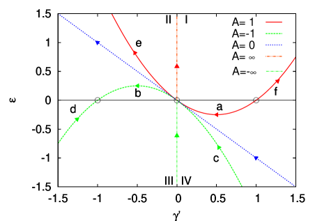
Figure 1: Main types of RG paths when the deviation from FTG is given by a single eigenfunction as in (IV.40). The characteristic cases of $A=-1,0,1$ together with the limits $A=\pm\infty$ are plotted. Circles mark their intersections with the fixed line $\epsilon=0$. The segments a,b represent closed loops, c,d converge to FTG, whereas e,f diverge from it.

In what follows we will give some explicit examples for the different types of RG trajectories discussed in this subsection.

IV.1.4 Excursions in distribution space

We now illustrate the solution given in the previous subsection on the case of the returning invariant manifolds discussed in (i) of the previous subsection. If we start an excursion near the FTG distribution in a linearly unstable direction with $1\gg-\epsilon_{0}>0$ then the path will turn back to the FTG fixed point along the marginal direction. This corresponds to paths like (a) on Fig. 1. We shall prefer a parameterization of the trajectory such that the $s\to-\infty$ limit corresponds to $\gamma^{\prime}\to\gamma^{\prime}_{\mathrm{i}}>0$, so by (IV.18) we have $\gamma^{\prime}_{\mathrm{i}}=1/A>0$, it is the initial parameter, and also $\epsilon\to\epsilon_{\mathrm{I}}=0$. For $s\to\infty$ the path goes to the origin $\epsilon=\gamma^{\prime}=0$. There remains an arbitrariness in choosing the origin of the parameter $s$: we set it now such that at $s=0$ the $-\epsilon(s)$ attains its maximum. This happens at $\gamma^{\prime}_{0}=\gamma^{\prime}_{\mathrm{i}}/2$ where $\epsilon_{0}=-\gamma^{\prime}_{\mathrm{i}}/4$. Then from (IV.21) we get

$$s=\frac{1}{\gamma^{\prime}}-\frac{2}{\gamma^{\prime}_{\mathrm{i}}}+\frac{1}{\gamma^{\prime}_{\mathrm{i}}}\ln\left(\frac{\gamma^{\prime}_{\mathrm{i}}}{\gamma^{\prime}}-1\right).$$ (IV.22)

From this equation, the asymptotes of $\gamma^{\prime}(s)$ can be computed as

$$\gamma^{\prime}\approx\left\{\begin{array}[]{lll}\gamma^{\prime}_{\mathrm{i}}(1-e^{-|s|\gamma^{\prime}_{\mathrm{i}}}),&\mathrm{if}&s\to-\infty,\\ \dfrac{1}{s},&\mathrm{if}&s\to\infty.\\ \end{array}\right.$$ (IV.23)

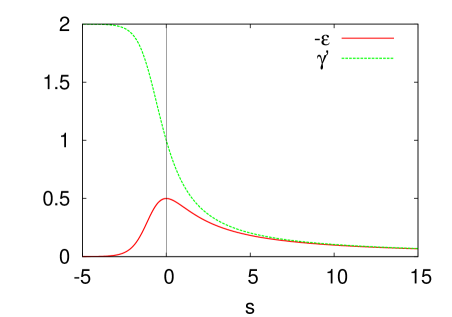
Figure 2: Amplitude $\epsilon$ and exponent $\gamma^{\prime}$ of the unstable manifold as function of the parameter $s$ for the case $\gamma^{\prime}_{\mathrm{i}}=2$.

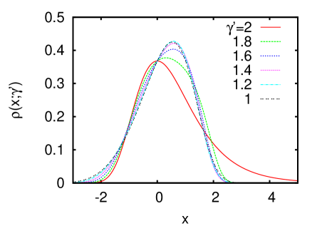
Figure 3: Probability densities (IV.24) of the unstable manifold with the parameters given in Fig. 2, during $s\leq 0$, i.e., $2\geq\gamma^{\prime}\geq 1$, where the amplitude of the perturbation $\epsilon$ grows. The numbers indicated are the $\gamma^{\prime}$ values, the initial value $\gamma^{\prime}_{\mathrm{i}}=2$ corresponds to the FTG distribution, and $\gamma^{\prime}=1$ to the farthest deviation from it measured in $\epsilon$. The parameters associated with the decreasing sequence of $\gamma^{\prime}$s are $s=-\infty,-1.543,-1.0681,-0.7094,-0.36950,0$ resp.

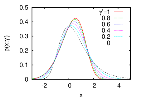
Figure 4: Same as in Fig. 3, but during $s\geq 0\,(0\leq\gamma^{\prime}\leq 1)$ where the amplitude of the perturbation $\epsilon$ decreases. The sequence begins at $\gamma^{\prime}=1$ and goes to $\gamma^{\prime}=0$, the latter corresponding to the FTG distribution because there $\epsilon=0$. The parameters associated with the decreasing sequence of $\gamma^{\prime}$s are $s=0,0.4527,1.0903,2.1931,5.0986,\infty$, resp.

Figure 2 displays the above obtained $\gamma^{\prime}(s)$ and $\epsilon(s)$ curves for $\gamma^{\prime}_{\mathrm{i}}=2$. We also illustrated the corresponding one-parameter family of probability densities as defined through (IV.1) by

$$\rho(x;\gamma^{\prime})=\partial_{x}\,e^{-e^{\scriptstyle-g(x,s(\gamma^{\prime}))}}.$$ (IV.24)

First we start out from the very proximity of the FTG distribution and move farther from it, a sequence up to $s=0$ is shown on Fig. 3, then for positive parameters $s>0$ the $\epsilon$ turns back towards zero and eventually the FTG distribution is approached, as displayed on Fig. 4.

The other looping invariant manifold corresponds to the line segment (b) in Fig. 1. The solution is given by the same formula as (IV.22) but now with $\gamma_{\mathrm{i}}^{\prime}$ replaced by a $\gamma_{\mathrm{f}}^{\prime}<0$. While in the parameter plane a simple symmetry transformation relates segment (a) with (b), the distributions themselves are manifestly different due to the sign change of the perturbation. This is demonstrated on Fig. 5, where the functions are oppositely skewed than those in the excursion on Figs. 3,4.

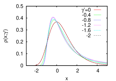
Figure 5: The unstable invariant manifold starting near the origin in parameter plane, corresponding to the path (b) in Fig. 1. While $\gamma^{\prime}$ changes from $0$ to $\gamma_{\mathrm{f}}^{\prime}=-2$ as marked in the legend, the distribution diverges from then converges to the FTG fixed point.

IV.1.5 Non-returning paths in distribution space

We shall illustrate paths not making excursions from and to FTG, as described in paragraphs (ii) and (iii) of subsection IV.1.3. The solution (IV.18,IV.21) is valid, with semi-infinite support for $\epsilon\neq 0$, whence the continuous part $\rho_{\mathrm{c}}(x;\gamma^{\prime})$ of the probability density function can be reconstructed.

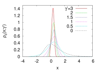
Figure 6: Continuous part of the density for the trajectory starting in quarter IV in parameter plane and converging to FTG, as it corresponds to the path (c) in Fig. 1. The integral of this function is less than one, except in the FTG limit $\gamma^{\prime}=0$. Characteristic values of $\gamma^{\prime}$ of the distributions are displayed, converging to zero while $s\to\infty$.

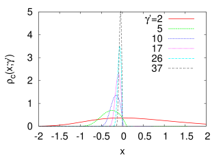
Figure 7: Continuous part of the density for the trajectory starting in quarter I and diverging in the parameter plane, as it corresponds to the path (f) in Fig. 1. The integral of this function is less than one, except in the FTG limit, obtained by backtracking for $s\to-\infty$. Characteristic values of $\gamma^{\prime}$ of the distributions are displayed, where $\gamma^{\prime}=2$ corresponds to FTG, as seen from Fig. 1.

First we consider a path corresponding to the segment (c) of Fig. 1, where (IV.3) gives a finite lower border $x_{\ast}$ for $\gamma^{\prime}>0$. Then the continuous part of the density $\rho_{\mathrm{c}}(x;\gamma^{\prime})$ vanishes at $x_{\ast}$ and has a norm smaller than one, as illustrated by the sequence in Fig. 6. As explained in Sec. IV.1.1 we associate a complementary discrete probabilistic weight with $x_{\ast}$. This weight, never exceeding $1/e$ and vanishing in the FTG limit, could be represented by a Dirac delta in the density, but we omit it from the figure. Secondly, we illustrate in Fig. 7 a trajectory of the segment (f) of Fig. 1, where (IV.3) gives a finite upper border $x^{\ast}$. For $s\to-\infty$ we have the FTG limit, and for increasing $s$ the $x^{\ast}$ decreases and reaches zero. This happens at a finite $s$, as it can be seen from (IV.21), corresponding to the point at infinity along the parabola segment (f) on Fig. 1. In this limit the non-normalized part of the distribution becomes peaked at the origin, and, together with the discrete weight at the upper border of the support (not shown on Fig. 7), form a Dirac delta at the origin. This single weight is the generic EVS limit distribution when the parent has a discrete weight at the upper border of the support, and formally corresponds to the $\gamma\to-\infty$ limit of the FTW fixed point distribution.

The above illustrated cases are the typical non-returning trajectories, converging ones go to FTG, while diverging ones in the plane represent convergence to a Dirac delta.

This ends our examples where a single eigenfunction, appropriately parameterized, gives exactly the RG path even farther away from the FTG fixed point.

IV.2 RG flow in terms of the general linearized solution around FTG

IV.2.1 Reparameterization of the general solution of the linearized PDE

Given the RG trajectories in the previous subsection IV.1, whose functional form is characterized by a single eigenfunction, it is natural to ask whether the solution could be generalized to linear combinations of the eigenfunctions. In other words, assuming the form of the general linearized solution as described in Sec. III.4.4, for the FTG case, the question is whether we can parameterize it appropriately such that it provides exact RG paths.

Considering the explicit form of the FTG eigenfunction (III.47), one sees that $\gamma^{\prime}$ acts as a rescaling of the variable $x$, as well as a global rescaling factor of the function $\psi$. Noticing that the variations of this global rescaling factor can be reabsorbed into $\epsilon$ through a suitable redefinition of $s$, we conclude that the ansatz (IV.1) is equivalent to a rescaling of $x$ together with a reparameterization of $s$. This suggests to use the following more general ansatz, where the eigenfunction is now replaced by a general solution $\phi$ of the linearized equation as

$$g(x,s)=x+\phi\big{(}\beta(s)x,\eta(s)\big{)},$$ (IV.25)

where $\beta(s)$ and $\eta(s)$ are functions to be determined, and $\phi$ is defined in (III.48) for $\gamma=0$ as

$$\phi(x,s)=\chi(s)+x\chi^{\prime}(s)-\chi(x+s).$$ (IV.26)

Inserting the above form of $g(x,s)$ into the PDE (III.15) yields a set of two coupled differential equations for $\beta(s)$ and $\eta(s)$:

$$\dot{\eta} =\beta,$$ (IV.27a)

$$\dot{\beta} =\beta^{3}\chi^{\prime\prime}(\eta).$$ (IV.27b)

Consequently, the ansatz (IV.25,IV.26) is an exact RG trajectory if the running parameters satisfy the above ODE’s. This is remarkable if one recalls that it represents an extension of the solution in the linear neighborhood of the FTG fixed point by only using a suitable parameterization. Even more remarkably, as we shall see it below, the present ansatz is actually the most general solution of the PDE for the RG flow, and the meaning of the parameter functions will also be revealed.

Before going on, we should note that the pair of ODE’s (IV.27) can be solved explicitly for the $\beta(\eta)$ and $s(\eta)$ functions with arbitratry initial conditions. We can obtain this solution by firstly dividing the two equations to yield an ODE for $\beta(\eta)$, which can be integrated, and secondly, by substituting the thus obtained $\beta(\eta)$ into (IV.27a), which then yields explicitly $s(\eta)$. Instead of displaying and analyzing this solution, however, we shall follow a different and perhaps more surprising reasoning.

IV.2.2 ODE’s for a general RG path

Let us reconsider the scale and shift parameters of the RG transformation, i.e., $a(s)$ and $b(s)$ of Sec. III.2. From their definition Eqs. (III.9,III.11) we obtain a pair of ODE’s

$$\dot{b} =a,$$ (IV.28a)

$$\dot{a} =-a^{3}\,g^{\prime\prime}(b),$$ (IV.28b)

where we remind the reader that $g(x)=g(x,0)$ is the initial condition for the PDE, corresponds to the parent distribution, and meets the standardization conditions (III.6). The above equations are essentially the same as the formerly displayed (III.13,III.14). The initial condition of the scale and shift parameters is obviously $a(0)=1$ and $b(0)=0$.

Conversely, it is straightforward to show that the above pair of ODE’s, with the aforementioned initial condition, can be uniquely solved resulting in (III.9,III.11).

We can immediately recognize the similarity between the pairs of equations (IV.27) and (IV.28). There are still a few steps to make before the analogy is fully specified. First, we should set the initial conditions in (IV.27) to $\eta(0)=0$ and $\beta(0)=1$. Then, using these values, we obtain the initial function $g(x)$ in terms of $\chi(x)$ by substitution of (IV.26) into (IV.25) to yield

$$g(x)=g(x,0)=x+\chi(0)+x\chi^{\prime}(0)-\chi(x).$$ (IV.29)

Hence $g^{\prime\prime}(x)=-\chi^{\prime\prime}(x)$ and we see that the two sets of ODE’s (IV.27) and (IV.28) are identical. Therefore, the correspondence

$$\eta(s) =b(s)=g^{-1}(s)$$ (IV.30a)

$$\beta(s) =a(s)=1/g^{\prime}\big{(}\eta(s)\big{)}$$ (IV.30b)

holds. Eventually, it remains to be clarified what the role of the $\eta$ and $\beta$ parameters in formula (IV.25) for the RG flow is. While the parameters $a(s)$ and $b(s)$ enter as the respective scale and shift in the argument of (III.8), at first glance it is not obvious that also $\eta$ and $\beta$ in (IV.25) define a linear transformation. We start out from (III.8), substituting the function $g(x)$ from (IV.29) and $s(\eta)$ from the inversion of (IV.30a). This yields

$$g(x,s)= g\big{(}\beta(s)x+\eta(s)\big{)}-s$$

$$= \beta x+\eta+\chi(0)+(\beta x+\eta)\chi^{\prime}(0)-\chi(\beta x+\eta)$$

$$-\eta-\eta\chi^{\prime}(0)-\chi(0)+\chi(\eta)$$

$$= \beta x\big{(}1+\chi^{\prime}(0)\big{)}+\chi(\eta)-\chi(\beta x+\eta).$$ (IV.31)

Equations (IV.29) and (IV.30b) have the consequence

$$\beta\big{(}1+\chi^{\prime}(0)\big{)}=1+\beta\chi^{\prime}(\eta),$$ (IV.32)

which can be substituted into (IV.31) to yield

$$\begin{split}g(x,s)=&x+\beta x\chi^{\prime}(\eta)+\chi(\eta)-\chi(\beta x+\eta)\\ =&x+\phi(\beta x,\eta).\end{split}$$ (IV.33)

The last line is obtained by the definition (IV.26), whereby the starting ansatz (IV.25) is recovered.

In summary, the trial function (IV.25) includes the most general, defining formula (III.8) for the RG trajectories. A direct derivation of this conclusion, without using the differential formalism, is presented in Appendix A. One should recall that the function $\chi(x)$ in (IV.26), if small, is related to the weight in a linear combination of eigenfunctions, as seen in Sec. III.4. In fact, the motivation for (IV.25) was to construct a generalization of the solution in the linear neighborhood of the FTG fixed point, valid also in the non-perturbative regime, i.e., for not only small $\chi(x)$. While the RG paths in terms of a single eigenfunction about FTG, as discussed in Sec. IV.1, could be considered as a curiosity, now we see that the RG transformation generally maintains the functional form also for linearly weighted combination of eigenfunctions, if appropriately parameterized, even farther from the FTG fixed point. This is to our knowledge a very special property for an RG transformation, unparalleled over its areas of applications in statistical physics.

IV.2.3 ODE’s for the perturbation parameter

In order to make a connection with the single eigenfunction case, as well as to explicitly characterize the deviation from the FTG fixed point, a perturbation amplitude $\epsilon$ can be introduced for a general RG trajectory. With the notation of Sec. IV.2.1 let us define

$$\epsilon=\beta^{2}\chi^{\prime\prime}(\eta).$$ (IV.34)

Hence we can rewrite (IV.27b) as

$$\dot{\beta}=\epsilon\,\beta.$$ (IV.35)

Taking the derivative of (IV.34) with respect to $s$, we get using the pair of ODE’s (IV.27)

$$\dot{\epsilon}=2\epsilon^{2}+\beta^{3}\,\chi^{\prime\prime\prime}(\eta).$$ (IV.36)

Then reexpressing $\eta$ from (IV.34), we can write $\dot{\epsilon}$ as a function of $\epsilon$ and $\beta$ only

$$\dot{\epsilon}=2\epsilon^{2}+\beta\,\epsilon\,\varphi(\epsilon/\beta^{2}),$$ (IV.37)

where we have introduced the auxiliary function

$$\varphi(y)=\frac{\chi^{\prime\prime\prime}(\chi^{\prime\prime-1}(y))}{y}.$$ (IV.38)

The ODE’s (IV.35,IV.37) can be considered as the generalization of (IV.11), valid for RG paths in terms of a single eigenfunction. The latter is recovered as a special case in the following way. Consider the initial conditions $\beta(0)=1$, $\gamma^{\prime}(0)=\gamma_{0}^{\prime}$, and $\epsilon(0)=\epsilon_{0}$, then identify $\gamma^{\prime}$ with $\beta\gamma_{0}^{\prime}$, choose $\chi(x)$ so that $\chi^{\prime\prime}(x)=\epsilon_{0}e^{\gamma_{0}^{\prime}x}$ yielding $\varphi(y)\equiv\gamma_{0}^{\prime}$, thus we are led back to (IV.11).

Note that the parameter $\epsilon(s)$ introduced above equals the “effective” $\gamma(s)$ of (III.14), and can be considered as a measure of the deviation from the FTG fixed point in the general case, not only when a deviation is represented by a single eigenfunction.

IV.2.4 An example

We shall illustrate the RG paths as given in the previous part of Sec. IV.2 on an example for an excursion from the FTG fixed point. Note that returning invariant manifolds were, remarkably, given in closed forms in Sec. IV.1. The example shown here can be considered as a generalization of them. Consider a linear combination of unstable eigenfunctions, weighted uniformly between $\gamma^{\prime}=0$ and a $\gamma^{\prime}_{0}>0$, corresponding to

$$\chi(x)=\frac{3\epsilon_{0}}{\gamma_{0}^{\prime 3}}\int_{0}^{\gamma_{0}^{\prime}}e^{\gamma^{\prime}x}d\gamma^{\prime}=\frac{3\epsilon_{0}}{\gamma_{0}^{\prime 3}}\frac{e^{\gamma_{0}^{\prime}x}-1}{x}.$$ (IV.39)

Note that the constant $\gamma^{\prime}_{0}$ now is not to be confounded with an initial condition, rather it is the upper border of set of $\gamma^{\prime}$ indices here.

Choosing $\chi(x)$ as given in (IV.39) yields through (IV.29) a parent $g(x)$ with support extending to the real axis, if $2\gamma_{0}^{\prime}>-3\epsilon_{0}>0$. The scale and shift parameters $\beta=a$, $\eta=b$ are determined through (IV.30) and the perturbation parameter $\epsilon$ through (IV.34). This is illustrated on Fig. 8 whose qualitative similarity with Fig. 2 is apparent. While this example is about a case when the support is the real axis, the general formulas in this section also describe cases with limited support, similarly to the situation when the deviation from the FTG fixed point was given in terms of a single eigenfunction, as discussed in Sec. IV.1.

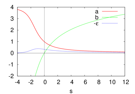
Figure 8: Excursion from FTG starting from a linear combination of eigenfunctions. In (IV.29) the function (IV.39) with $\epsilon_{0}=-1/2$ and $\gamma_{0}^{\prime}=1$ was taken. The running parameters $a(s)=\beta(s)$ and $b(s)=\eta(s)$ in (IV.30), and the effective $\epsilon(s)$ defined in (IV.37) are displayed. Note that while Fig. 2 characterizes single invariant manifolds, these curves parameterize a continuum bundle of manifolds. The corresponding probability density function sequence first diverges from then converges to the FTG fixed point, in a manner qualitatively similar to the sequences displayed in Figs. 3,4.

IV.3 Paths about the FTF and FTW fixed points in terms of single eigenfunctions

IV.3.1 Trial functions for the RG path

It is a natural question to ask whether a generalization of the ansatz (IV.1) in terms a single eigenfunction may give trajectories belonging to fixed points other than the FTG one. We propose such a generalization in the form of the trial function

$$g(x,s)=f\Big{(}x+\epsilon(s)\psi\big{(}x;\bar{\gamma}(s),\gamma^{\prime}(s)\big{)};\bar{\bar{\gamma}}(s)\Big{)},$$ (IV.40)

where the fixed point function $f$ is given by (III.26), the eigenfunction $\psi$ by (III.46), and the running parameters $\epsilon(s),\bar{\gamma}(s),\gamma^{\prime}(s),\bar{\bar{\gamma}}(s)$ are to be determined from the PDE (III.15). We used here the notation $\bar{\gamma}(s)$ and $\bar{\bar{\gamma}}(s)$ to distinguish them from the “effective” $\gamma(s)$ given in (III.19). While the $\bar{\gamma}$ should be equal to $\bar{\bar{\gamma}}$ for a proper eigenfunction about the fixed point with $\bar{\bar{\gamma}}$, we allow them to be different for the present trial function.

After substitution into the PDE (III.15) a somewhat tedious but straightforward calculation shows that such a proposition can be valid only if

$$\bar{\bar{\gamma}}(s) =\gamma_{0},$$ (IV.41a)

$$\gamma^{\prime}(s) =B\,\bar{\gamma}(s),$$ (IV.41b)

where $\gamma_{0}$ and $B$ are constants. Thus the ansatz reduces to

$$g(x,s)=f\Big{(}x+\epsilon(s)\psi\big{(}x;\bar{\gamma}(s),B\bar{\gamma}(s)\big{)};\gamma_{0}\Big{)},$$ (IV.42)

wherein two running parameters remained. These, again by (III.15), can be shown to lead to an RG path if they satisfy the ODE’s

$$\dot{\epsilon} =2\epsilon^{2}+\epsilon(\gamma_{0}+(B-1)\bar{\gamma}),$$ (IV.43a)

$$\dot{\bar{\gamma}} =\bar{\gamma}(\epsilon+\gamma_{0}-\bar{\gamma}).$$ (IV.43b)

Consistency with the flow about the FTG fixed point can be checked, if we take $B\to\infty$ while keeping $\gamma^{\prime}(s)$ in (IV.41b) finite, and set $\gamma_{0}=0$, when we immediately recover the pair of ODE’s in (IV.11).

An interesting feature emerges if we keep $\gamma_{0}$ nonzero while $B\to\infty$. Then starting near the non-FTG fixed point $f(x;\gamma_{0})$ but using an eigenfunction belonging to FTG, $\psi(x;0,\gamma^{\prime}(s))$, also leads to an exact, nonperturbative RG path in function space.

Another remarkable property of the ansatz (IV.42) is that it can also describe fixed points corresponding to $\gamma\neq\gamma_{0}$. Indeed, it is straightforward to show that

$$f(x;\gamma+\epsilon)=f(x+\epsilon\psi(x;\gamma+\epsilon,-\epsilon);\gamma),$$ (IV.44)

which can be considered as a special structural relation between the fixed point functions and the eigenfunctions.

IV.3.2 Fixed points and flow lines in parameter plane

In what follows we shall briefly review some basic properties of the above ODE’s. There are in general four fixed points for nonzero $\gamma_{0}$.

(i) $\epsilon^{\ast}=\bar{\gamma}^{\ast}=0$, corresponding to the fixed point function $f(x;\gamma_{0})$.

(ii) $\epsilon^{\ast}=0$, $\bar{\gamma}^{\ast}=\gamma_{0}$, again with $f(x;\gamma_{0})$.

(iii) $\epsilon^{\ast}=-\gamma_{0}/2$, $\bar{\gamma}^{\ast}=0$, with $f(x;\gamma_{0}/2)$.

(iv) $\bar{\gamma}^{\ast}=\gamma_{0}/(B+1)$, $\epsilon^{\ast}=-B\bar{\gamma}^{\ast}$, with $f(x;\gamma_{0}/(B+1))$. Note that in (iii-iv) the fixed point functions $f(x;\gamma)$ with $\gamma\neq\gamma_{0}$ arise as made possible by the special property (IV.44).

For general flow lines in the parameter plane $\bar{\gamma},\epsilon$ an ODE is obtained from (IV.43) as

$$\epsilon^{\prime}(\bar{\gamma})=\frac{2\epsilon}{\bar{\gamma}}+\frac{\epsilon}{\bar{\gamma}}\frac{\bar{\gamma}(B+1)-\gamma_{0}}{\epsilon+\gamma_{0}-\bar{\gamma}}.$$ (IV.45)

Some invariant lines can be explicitly found as follows.

(a) $\epsilon\equiv 0$ corresponding to staying at $f(x;\gamma_{0})$.

(b) $\bar{\gamma}\equiv 0$ implying a flow by $\dot{\epsilon}=2\epsilon^{2}+\epsilon\gamma_{0}$, and containing the fixed points (i,iii).

(c) $\epsilon=-B\bar{\gamma}$, along which we have $\dot{\bar{\gamma}}=\bar{\gamma}(\gamma_{0}-(B+1)\bar{\gamma})$, containing the fixed points (i,iv).

(d) $\epsilon=(B+1)\bar{\gamma}(\bar{\gamma}/\gamma_{0}-1)$, containing the fixed points (i,iii,iv).

For graphical illustration let us restrict ourselves to positive $\gamma_{0}$ and $B$. Then all fixed points lie in the fourth quarter of the parameter plane with $\bar{\gamma}\geq 0$, $\epsilon\leq 0$, the (i) is unstable, (ii,iii) are saddle points, and (iv) is stable. The latter attracts all RG trajectories starting within the quarter plane with $\bar{\gamma}>0$, $\epsilon<0$. On Fig. 9, we display some characteristic flow lines. The main difference with respect to the RG paths about the FTG fixed point is that in this example we do not have excursions, rather, the RG transformation connects different fixed points.

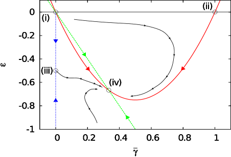
Figure 9: RG flow in $\bar{\gamma},\epsilon$ space, when the deviation from the FTF fixed point with $\gamma_{0}=1$ is given by a single eigenfunction as in (IV.42), with $B=2$. Circles mark the fixed points (i-iv) listed in the text, and invariant curves of the simple types (b-d) as well as some qualitatively drawn flow lines are indicated.

IV.3.3 Examples

In order to highlight the above observations we give two families of solutions. On the one hand, the family

$$g(x,s)=f\left(x+\frac{\epsilon}{\gamma^{\prime 2}}\left(1+\gamma^{\prime}x-e^{\gamma^{\prime}x}\right);\gamma_{0}\right)$$ (IV.46)

corresponds to $B\to\infty$ while $B\bar{\gamma}=\gamma^{\prime}$ and so from (IV.43) the ODE’ become

$$\dot{\epsilon} =2\epsilon^{2}+\epsilon(\gamma_{0}+\gamma^{\prime}),$$ (IV.47a)

$$\dot{\gamma^{\prime}} =\gamma^{\prime}(\epsilon+\gamma_{0}).$$ (IV.47b)

Note that this is the generalization of (IV.11) to nonzero $\gamma_{0}$. As the second example we display the RG path along the invariant line $\epsilon=-B\bar{\gamma}$ for which, after some rearrangements, we get

$$g(x,s)=f\left(\frac{(1+\bar{\gamma}x)^{B+1}-1}{\bar{\gamma}(1+B)};\gamma_{0}\right).$$ (IV.48)

The running parameter $\bar{\gamma}(s)$ satisfies the ODE given under paragraph (c). These two examples demonstrate manifestly that eigenfunctions of some fixed point composed with another fixed point function can lead to exact trajectories.

IV.3.4 Paradox: can a fixed point with an eigenfunction of another fixed point be a solution?

We end this part by calling the reader’s attention to a seemingly paradoxical situation, namely, that (IV.42) contains a fixed point function with parameter $\gamma_{0}$, while the eigenfunction within can have, and typically has, a different $\bar{\gamma}\neq\gamma_{0}$ parameter. Then the question arises, how a solution near a fixed point, i.e. having a small $\epsilon$ can be expressed in terms of a non-proper eigenfunction. The resolution of that is simple: If the eigenfunction contains parameters changing in $s$ then it may be of the functional form of the eigenfunction, but the perturbation in the argument corresponding to (III.28) does not separate as (III.36) into an $s$- and $x$-depending function. So the eigenfunction with changing parameters is not a solution of the eigenvalue problem, thus there is no contradiction with the known solutions. Only if the $s$-dependence of the parameter $\bar{\gamma}$ in (IV.42) is negligible (vanishing with $\epsilon$) will we obtain separability as in (III.36). The parameter $\bar{\gamma}$ can change slowly only near fixed points in the parameter plane, among which we are interested now in (i) and (ii) located on the $\epsilon=0$ axis. But then near the fixed point (i) the eigenfunction becomes $\psi\big{(}x;\bar{\gamma}(s),B\bar{\gamma}(s)\big{)}\approx-x^{2}/2$, a valid eigenfunction of $f(x;\gamma_{0})$ of index $\gamma^{\prime}=\gamma_{0}$, furthermore, near the fixed point (ii) the parameter $\bar{\gamma}(s)\approx\gamma_{0}$ so again we are facing a proper eigenfunction (with $\gamma^{\prime}=B\gamma_{0}$). In summary, the exact solution (IV.42) does not include a case where an improper eigenperturbation would appear.

V RG for central limit distributions

In this section we demonstrate a remarkable albeit simple analogy between limiting behavior in EVS and central limit distributions. So far we have studied the RG transformation that arose from the EVS problem, as discussed in Secs. II and III. In its original form (III.1) the transformation consists of a linear change of variable and raising the distribution function to a power. It is well known, however, that formally a similar operation, rescaling and raising to power, should be performed also in the context of the central limit problem on the moment generating function Gnedenko and Kolmogorov (1954); Christoph and Wolf (1993). In this section we briefly review this similarity and show that some of the so far considered RG fixed points actually correspond to distributions known as “stable”, i.e., having the property that sums of random variables keep the same distribution up to a scale transformation. The main idea of the RG for distributions falling into the Gaussian class has been expounded in Jona-Lasinio (2001), treated as an introductory example, where the eigenvalue problem for analytic characteristic functions has also been determined.

Below we show that the RG flow equation introduced in this paper for EVS leads, with a slightly different standardization, to a PDE whose fixed point solution corresponds to central limit distributions. We restrict ourselves for the sake of simplicity here to real, symmetric moment generating functions, so the fixed point will describe probability densities with even symmetry. We also evaluate the eigenfunctions and again find a close similarity to those found in EVS.

V.1 RG transformation

Consider the random variable $Z$ defined as a rescaled sum of random variables, namely

$$Z=\frac{1}{a_{N}}\sum_{i=1}^{N}z_{i},$$ (V.1)

where $z_{i}$ are i.i.d. numbers each with density $P(z)$ and moment generating function

$$\Phi(q)=\int_{-\infty}^{\infty}\mathrm{d}z\,e^{iqz}\,P(z),$$ (V.2)

and $a_{N}$ is a suitable scaling factor ensuring a non-degenerate limit distribution, if such exists. We assume that $P(z)=P(-z)$, which implies $\langle z\rangle=0$. From the parity of $P(z)$, we also have that the moment generating function $\Phi(q)$ is real, and satisfies $\Phi(q)=\Phi(-q)$. Then the moment generating function for the variable $Z$ is known to be

$$\Phi_{N}(q)=\Phi^{N}(a_{N}q),$$ (V.3)

also real and symmetric. Allowing a continuation of $N$ and introducing $s=\ln N$ we suitably define a RG transformation on the moment generating function as

$$\Phi(q,s)=[\hat{R}_{s}\Phi](q)=\Phi^{e^{s}}\!\big{(}a(s)\,q\big{)}.$$ (V.4)

An alternative interpretation of the RG would also be to perform a decimation operation, similarly to the procedure presented in Sec. II for EVS. The function $\Phi(q,s)$ is real and even in $q$, and is related to the corresponding probability density by a Fourier transformation like in (V.2). While $\Phi(0,s)\equiv 1$ follows from (V.2), we have the freedom to impose a standardization condition, which sets the scale factor $a(s)$, so we require

$$\Phi(1,s)=\Phi(-1,s)\equiv e^{-1}.$$ (V.5)

The above transformation is in clear analogy to the RG operation for EVS (III.7), but while RG acted on the integrated distribution function there, here its argument is the moment generating function. Note the difference in standardization: in EVS the distribution function became $1$ at the upper limit of the support and was $e^{-1}$ at $x=0$, now $1$ is reached in the origin and $e^{-1}$ at $q=-1$. Another difference is that we do not have a monotonicity condition in $q$ here, nonetheless, the analogy between (III.7) and (V.4) is obvious.

To further emphasize the similarity to the RG equation in EVS, we introduce the function $h(q,s)$ by

$$\Phi(q,s)=e^{-e^{\scriptstyle-h(q,s)}}.$$ (V.6)

Then $h(q)=h(q,0)$ corresponds to the starting moment generating function $\Phi(q)=\Phi(q,0)$. Since $h(q,s)$ is even in $q$, it suffices to only consider one semi-axis in $q$. To prepare for the analogy to EVS, we shall consider the negative semi-axis, i.e. $q<0$. The RG transformation (V.4) implies

$$h(q,s)=h\big{(}a(s)\,q\big{)}-s.$$ (V.7)

From $\Phi(0,s)\equiv 1$ and the standardization (V.5) follow

$$h(0,s) \equiv\infty,$$ (V.8a)

$$h(-1,s) \equiv 0,$$ (V.8b)

the latter setting the scale parameter by (V.7) as

$$h(-a(s))=1+s.$$ (V.9)

Differentiation of (V.7) by both variables yields

$$\partial_{s}h(q,s) =q\,\dot{a}(s)\,h^{\prime}(a(s)q)-1,$$ (V.10a)

$$\partial_{q}h(q,s) =a(s)\,h^{\prime}(a(s)q).$$ (V.10b)

Hence we obtain the PDE for $h$ as

$$\partial_{s}h(q,s)=q\,\gamma(s)\,\partial_{q}h(q,s)-1,$$ (V.11)

where

$$\gamma(s)=\frac{\dot{a}(s)}{a(s)}.$$ (V.12)

The standardization condition (V.5) implies that the left-hand-side of the (V.11) is zero at $q=-1$, whence

$$\gamma(s)=-\frac{1}{\partial_{q}h(-1,s)}.$$ (V.13)

Thus we wound up in (V.11) with a nonlinear PDE, which resembles the PDE (III.15) obtained for the EVS problem, while the analog of (V.13) is (III.19). The difference can be ascribed to the modified standardization.

V.2 Fixed point

Fixed point functions for the PDE above can be found by looking for $s$-independent solutions $h(q,s)\equiv f(q)$ with a constant $\gamma(s)\equiv\gamma$. From (V.11) we obtain

$$q\,\gamma\,f^{\prime}(q)=1,$$ (V.14)

whence the solution for $q<0$, satisfying the standardization $f(-1)=0$, is

$$f(q;\gamma)=\frac{1}{\gamma}\ln(-q).$$ (V.15)

Hence the moment generating function in the fixed point is by (V.6)

$$\Phi(q;\gamma)=e^{-(-q)^{-\frac{1}{\gamma}}}.$$ (V.16)

This is precisely of the form of the FTW distribution with $\gamma<0$ originally obtained by Fisher and Tippett Fisher and Tippett (1928). Now this function corresponds to the moment generating function of the stable distributions with even symmetry, usually written as

$$\Phi_{\alpha}(q)=e^{-|q|^{\alpha}},$$ (V.17)

with $0<\alpha\leq 2$. By identification, we thus get $\alpha=-1/\gamma$. The restriction for $\alpha$ is imposed to have a valid probability density in the relation (V.2), $\alpha=2$ corresponding to a Gaussian and $\alpha<2$ to the Lévy family. Note that the validity of the moment generating function (namely, its inverse Fourier transform should be a positive function) is in itself not ensured for any solutions of the PDE (V.11), but the PDE preserves validity if the initial condition was appropriate.

In conclusion, we obtained the even limit distributions for the sum of i.i.d. random variables in terms of their moment generating function, which is on the negative semi-axis identical to the FTW family of limit distributions in EVS. The correspondence holds with $\alpha=-1/\gamma$, where $\alpha$ is the Lévy index and $\gamma$ the parameter of the FTW distribution, in the region $\gamma\leq-1/2$.

V.3 Eigenfunctions

Again in analogy to the EVS problem, we can ask about the eigenfunctions of the RG transformation near a fixed point. Consider perturbing the fixed point function (V.15), whose second argument $\gamma$ we shall omit while assuming it fixed, as

$$h(q,s)=f\big{(}q+\epsilon(s)\,\psi(q)\big{)}\approx f(q)+\epsilon(s)f^{\prime}(q)\,\psi(q).$$ (V.18)

The symmetry of $h(q,s)$ in $q$ requires the function $\psi(q)$ to be odd, and standardization conditions will be imposed as

$$\psi(-1) =0,$$ (V.19a)

$$\psi^{\prime}(-1) =-\frac{1}{\gamma},$$ (V.19b)

whereby from (V.13) we obtain

$$\gamma(s)=\gamma+\epsilon(s)$$ (V.20)

Then substitution of (V.18) into the PDE (V.11) and linear expansion in $\epsilon$ results in

$$\dot{\epsilon}(s)\psi(q)=\epsilon(s)\big{(}q-\gamma\,\psi(q)+q\,\gamma\,\psi^{\prime}(q)\big{)}.$$ (V.21)

This can be solved for nonzero $\epsilon$ only if

$$\frac{\dot{\epsilon}(s)}{\epsilon(s)}=\gamma^{\prime}$$ (V.22)

is a constant, whence we obtain

$$\gamma^{\prime}\psi(q)=q-\gamma\,\psi(q)+q\,\gamma\,\psi^{\prime}(q).$$ (V.23)

The solution meeting the conditions (V.19) is straightforwardly obtained, for $q<0$ it is

$$\psi(q;\gamma,\gamma^{\prime})=\frac{1}{\gamma^{\prime}}\left(q+(-q)^{(\gamma+\gamma^{\prime})/\gamma}\right).$$ (V.24)

Extending for all $q$’s with odd symmetry, and using the Lévy index $\alpha$ and the notation $\delta=-\alpha\gamma^{\prime}$ we eventually arrive at

$$\psi_{\alpha,\delta}(q)=-\frac{\alpha q}{\delta}\left(1-|q|^{\delta}\right).$$ (V.25)

Note the similarity of the eigenfunction with the one obtained for the EVS problem (III.46): both are essentially power functions with a linear function added to meet standardization. In particular, the function (V.24) is obtained from (III.46) in the FTW case with a suitable shift and rescaling.

The present treatise of the RG for the central limit problem is only meant to be a demonstration of the close similarity with EVS. While it can have further consequences for convergence to the limit, possible exact solutions of the RG equation, and generalization to non-symmetric distributions, we relegate those to further studies.

VI Conclusion and outlook

The RG transformation for the EVS problem can be considered a simple if not the simplest nonlinear RG conceivable: it consists of raising the integrated distribution function to a power and applying a linear change of the random variable. This gave rise to a linear, first order PDE, albeit with a parametric driving determined by the parent distribution, or equivalently, the initial condition. On the other hand, the coefficient can also be viewed as the curvature of the solution in the origin, which makes the PDE nonlinear but without an external forcing term. The versatility of the PDE is reflected by the fact that it can also account for discontinuities in the integrated distribution function.

The PDE approach allowed for a quite short and straightforward derivation of the fixed line of limit distributions and of the eigenfunctions. Furthermore, we found various exact solutions for the RG path in terms of fixed points and eigenfunctions, i.e., invariant manifolds, valid arbitrarily far from the fixed point. In general, we found that all solutions, extending also to the nonlinear region away from the fixed line, can be interpreted as linear combinations of eigenfunctions with possibly continuous weights. We suggest that this peculiar structure of function space, unparalleled in other RG methods in statistical physics, is the consequence of the extreme simplicity of the RG operation. An analogous RG operation in terms of a PDE could also be defined for the central limit problem, but on the moment generating function rather than the integrated distribution, and it allowed the simple rederivation of the known, even, Lévy stable functions as well as the calculation of eigenfunctions.

There is a plethora of further directions worth pursuing. The most obvious application of the RG theory, not discussed in this paper, is to calculate finite size effects (see Györgyi et al. (2010)). While the limit distributions for the EVS problem of two random variables are known, having more intricate properties than the above studied single variable case, an RG approach there may be useful to reveal finite size effects. Other natural extensions to the statistics of higher order maxima and order statistics in general are also conceivable. Whereas there have been many advances thus far for the EVS of various problems of correlated variables, especially in random walks, extensions of the RG concept again may prove to be useful. In fact, in a multitude of problems in the broader field of front propagation, like random fragmentation, extremal paths on trees, and randomly generated binary trees, functional recursions and fixed point conditions are known. Extensions of them to appropriate RG pictures and their eigenvalue analysis holds the potential that finite size relaxation effects can be described in terms of eigenfunctions. Another generalization of the EVS paradigm for i.i.d. variables exists to cases where the batch size is large but is itself a random variable. Here the finite size effects can presumably be studied again with the help of the RG results. Finally, the formal analogy with the central limit problem holds the promise of a simple approach to finite size effects there as well.

Appendix A Relation between alternative forms of the RG equations

Whereas this paper presents, and focuses on, the differential representation of the RG transformation for EVS, it is insightful to perform a direct, non-differential treatment. Thus we reanalyze the relationship of the parameterization (IV.25) with the original, defining formula of the RG transformation, which is essentially based on shift and rescaling operations. This way we again demonstrate that the two formulations are equivalent. We begin our reasoning by reconsidering the linearized RG transform by a direct formulation.

So far in the paper, linear analysis of the RG has been based on the linearization of the PDE. An alternative approach is to linearize directly the RG transform (III.8), which was followed in Györgyi et al. (2008, 2010) in the calculation of eigenfunctions, a treatment we develop below. We consider a perturbation $\phi(x,s)$, like in Sec. IV.2.1, defined by

$$g(x,s)=x+\phi(x,s),$$ (A.1)

the corresponding parent being denoted as

$$g(x)=x+\phi_{0}(x)$$ (A.2)

Starting from (III.8) we get for the RG transform

$$x+\phi(x,s)=a(s)x+b(s)+\phi_{0}\big{(}a(s)x+b(s)\big{)}-s$$ (A.3)

Assuming that $\phi=\phi_{\mathrm{lin}}$ is small, one gets by linearizing (III.9) that $b(s)=s-\phi_{0}(s)$. Similarly, (III.13) yields $a(s)=\dot{b}(s)=1-\phi_{0}^{\prime}(s)$. Inserting these expressions for $a(s)$ and $b(s)$ in the RG (A.3), and linearizing the resulting equation yields

$$\phi_{\mathrm{lin}}(x,s)=\phi_{0}(x+s)-x\phi_{0}^{\prime}(s)-\phi_{0}(s).$$ (A.4)

This is precisely the solution (IV.26) of the linearized PDE in the FTG case, with $\phi_{0}(x)=-\chi(x)$. Hence this solution can straightforwardly be obtained by linearizing the RG (III.8), rather than by linearizing the PDE and then looking for the generic solution.

The linearized RG transform (A.4) can be reformulated as

$$\phi_{\mathrm{lin}}(x,s)=\phi_{0}(x+s)+\bar{a}(s)x+\bar{b}(s),$$ (A.5)

where $\bar{a}(s)$ and $\bar{b}(s)$ determine the shift by a linear function, on $\phi_{\mathrm{lin}}$ that allows it to fulfill the standardization conditions

$$\phi_{\mathrm{lin}}(0,s)=0,\qquad\partial_{x}\phi_{\mathrm{lin}}(0,s)=0,$$ (A.6)

yielding

$$\bar{a}(s)=-\phi_{0}^{\prime}(s),\qquad\bar{b}(s)=-\phi_{0}(s).$$ (A.7)

In this way, the linearized RG clearly appears as a (constant-speed) translation of the variable $x$, followed by a shift by a linear function in order to restore the standardization conditions.

Let us now see how we can get the solution of the full RG from the linearized one in this framework. To this aim, we first reformulate the full RG in terms of the function $\phi(x,s)$ defined in (A.1), but this time without making any approximation. Rearranging (A.3) gives

$$\phi(x,s)=\phi_{0}\big{(}a(s)x+b(s)\big{)}+\big{(}a(s)-1\big{)}x+\big{(}b(s)-s\big{)},$$ (A.8)

as the general form of an RG trajectory.

Now let us use $\phi_{\mathrm{lin}}(x,s)$ obeying (A.5) and define a new trial function $\phi(x,s)$ through a rescaling of $x$ and a reparametrization of $s$, in the following way:

$$\phi(x,s)\equiv\phi_{\mathrm{lin}}\big{(}\beta(s)x,\eta(s)\big{)},$$ (A.9)

where the auxiliary functions $\beta(s),\eta(s)$ will be determined later. Note that this trial function satisfies the standardization conditions (A.6). We now wish to check whether $\phi(x,s)$ could possibly be a solution of the full RG (A.8). One has

$$\phi(x,s)=\phi_{0}(\beta x+\eta)+\bar{a}(\eta)\beta x+\bar{b}(\eta).$$ (A.10)

Comparison with (A.8) leads us to set the auxiliary functions as $\beta(s)=a(s)$ and $\eta(s)=b(s)$. Then the relations

$$a(s)-1 =\bar{a}\big{(}\eta(s)\big{)}\beta(s),$$ (A.11a)

$$b(s)-s =\bar{b}\big{(}\eta(s)\big{)},$$ (A.11b)

should also be satisfied, which is not a priori obvious. However, these relations define the shift of $\phi$ by a linear function, which ensures that $\phi$ fulfills the standardization condition. As the trial function $\phi$ by construction meets this standardization, (A.11) should necessarily be satisfied. This can also be checked explicitly as follows. On the one hand, since $\eta=b$, we know that $g(\eta)=s$, or from (A.2) equivalently

$$\eta+\phi_{0}(\eta)=s.$$ (A.12)

But this equation, when we take into account (A.7), turns out to be just (A.11b). Next, taking the derivative of (A.12) with respect to $s$ yields $\dot{\eta}+\phi_{0}^{\prime}(\eta)\dot{\eta}=1$. Recalling (III.13) we have $a=\dot{b}$, that is, $\beta=\dot{\eta}$, leading to

$$\beta+\phi_{0}^{\prime}(\eta)\beta=1,$$ (A.13)

which, by our using (A.7), turns out to be identical to (A.11a).

So we can conclude that the rather intuitively constructed trial function (A.9) indeed incorporates the most general formula (A.8) for the RG path, just what we wanted to show.

References

- Bouchaud and Mézard (1997) J.-P. Bouchaud and M. Mézard, J. Phys. A 30, 7997 (1997).
- Györgyi et al. (2003) G. Györgyi, P. C. W. Holdsworth, B. Portelli, and Z. Rácz, Phys. Rev. E 68, 056116 (2003).
- Le Doussal and Monthus (2003) P. Le Doussal and C. Monthus, Physica A 317, 140 (2003).
- Majumdar and Comtet (2004) S. N. Majumdar and A. Comtet, Phys. Rev. Lett. 92, 225501 (2004).
- Schehr and Majumdar (2006) G. Schehr and S. N. Majumdar, Phys. Rev. E 73, 056103 (2006).
- Krapivsky and Majumdar (2000) P. L. Krapivsky and S. N. Majumdar, Phys. Rev. Lett. 85, 5492 (2000).
- Gumbel (1958) E. J. Gumbel, Statistics of Extremes (Dover Publications, 1958).
- Katz et al. (2002) R. W. Katz, M. B. Parlange, and P. Naveau, Adv. Water Resour. 25, 1287 (2002).
- Sornette et al. (1996) D. Sornette, L. Knopoff, Y. Kagan, and C. Vannest, J. Geophys. Res. 101, 13883 (1996).
- Embrecht et al. (1997) P. Embrecht, C. Klüppelberg, and T. Mikosch, Modelling Extremal Events for Insurance and Finance (Springer, Berlin, 1997).
- Longin (2000) F. Longin, J. Bank. Finance 24, 1097 (2000).
- Fisher and Tippett (1928) R. A. Fisher and L. H. C. Tippett, Procs. Cambridge Philos. Soc. 24, 180 (1928).
- Gnedenko (1943) B. V. Gnedenko, Ann. Math. 44, 423 (1943).
- Galambos (1978) J. Galambos, The Asymptotic Theory of Extreme Value Statistics (John Wiley & Sons, 1978).
- von Mises (1954) R. von Mises, Amer. Math. Soc. (Providence, R.I.) (1954).
- Clusel and Bertin (2008) M. Clusel and E. Bertin, Int. J. Mod. Phys. B 22, 3311 (2008).
- Hall (1979) P. Hall, Journal of Applied Probability 16, 433 (1979).
- Hall (1980) P. Hall, Advances in Applied Probability 12, 491 (1980).
- de Haan and Resnick (1996) L. de Haan and S. Resnick, Annals of Probability 24, 97 (1996).
- de Haan and Stadtmüller (1996) L. de Haan and U. Stadtmüller, J. Australian Math. Soc. 61, 381 (1996).
- Györgyi et al. (2008) G. Györgyi, N. R. Moloney, K. Ozogány, and Z. Rácz, Phys. Rev. Lett. 100, 210601 (2008).
- Györgyi et al. (2010) G. Györgyi, N. R. Moloney, K. Ozogány, Z. Rácz, and M. Droz, Phys. Rev. E 81, 041135 (2010).
- Zinn-Justin (2007) J. Zinn-Justin, Phase Transitions and Renormalisation Group (Oxford University Press, 2007).
- Jona-Lasinio (2001) G. Jona-Lasinio, Phys. Rep. 352, 439 (2001).
- Schehr and Le Doussal (2010) G. Schehr and P. Le Doussal, Journal of Statistical Mechanics: Theory and Experiment 2010, P01009 (2010).
- Gnedenko and Kolmogorov (1954) B. V. Gnedenko and A. N. Kolmogorov, Limit Distributions for Sums of Independent Random Variables, Addison-Wesley series in Mathematics (Addison-Wesley, Cambridge, MA, 1954).
- Christoph and Wolf (1993) G. Christoph and W. Wolf, Convergence Theorems with a Stable Limit Law (Akademie-Verlag, Berlin, 1993).