Alternative Stable Scroll Waves and Conversion of Autowave Turbulence

Abstract

Rotating spiral and scroll waves (vortices) are investigated in the FitzHugh-Nagumo model of excitable media. The focus is on a parameter region in which there exists bistability between alternative stable vortices with distinct periods. Response Functions are used to predict the filament tension of the alternative scrolls and it is shown that the slow-period scroll has negative filament tension, while the filament tension of the fast-period scroll changes sign within a hysteresis loop. The predictions are confirmed by direct simulations. Further investigations show that the slow-period scrolls display features similar to delayed after-depolarisation (DAD) and tend to develop into turbulence similar to Ventricular Fibrillation (VF). Scrolls with positive filament tension collapse or stabilize, similar to monomorphic Ventricular Tachycardia (VT). Perturbations, such as boundary interaction or shock stimulus, can convert the vortex with negative filament tension into the vortex with positive filament tension. This may correspond to transition from VF to VT unrelated to pinning.

Orderly contraction of the heart is essential to pump blood efficiently. This order is imposed by electrical excitation waves propagating throughout the heart muscle. Abnormalities in the propagation of excitation waves, known as arrhythmias, are responsible for many cardiac pathologies. Particularly dangerous are re-entrant arrhythmias, where excitation waves circulate along closed pathways. Re-entrant excitation “vortices”, that are not attached to anatomical features, are spiral waves (in two dimensions) scroll waves (in three dimensions). As a rule, the rotation frequency and shape of a spiral wave is uniquely determined by local properties of the tissue. We investigate a region of parameters in a simplified mathematical model of excitation, in which two classes of vortices can exist. They differ significantly in their frequency and shape. Which of the two is realized, depends on the initial conditions. The defining feature of the model, responsible for this dichotomy, is well known in heart electrophysiology. It is called delayed after-depolarization and is known to have a pro-arrhythmic effect. We focus especially on the three-dimensional scroll waves. Based on the asymptotic theory utlizing Response Functions, we predict a change of sign of the filament tension of the scrolls on one of the branches. Negative tension is known to promote “scroll wave turbulence”. We investigate, by numerical simulations, specifics of this phenomenon in presence of alternative scrolls. We describe conversion of one type of vortex to the other under various perturbations, including external shocks such as are used for defibrillation, interactions with boundaries, and curvature of the scroll filaments. Finally, we discuss implications of our findings for cardiac arrhythmias.

I Introduction

Spiral waves in two-dimensions, and scroll waves in three-dimension, are regimes of self-organization observed in physical Frisch-etal-1994 ; Madore-Freedman-1987 ; Schulman-Seiden-1986 , chemical Zhabotinsky-Zaikin-1971 ; Jakubith-etal-1990 , and biological Allessie-etal-1973 ; Gorelova-Bures-1983 ; Alcantara-Monk-1974 ; Lechleiter-etal-1991 ; Carey-etal-1978 ; Murray-etal-1986 dissipative systems, where wave propagation is supported by a source of energy stored in the medium. The interest in the dynamics of these waves has significantly broadened over the years as developments in experimental techniques have permitted them to be observed and studied in an ever increasing number of diverse systems Shagalov-1997 ; Oswald-Dequidt-2008 ; Larionova-etal-2005 ; Yu-etal-1999 ; Agladze-Steinbock-2000 ; Bretschneider-etal-2009 ; Dahlem-Mueller-2003 ; Igoshin-etal-2004 . However, the occurrence of these waves in excitable media, and cardiac tissue in particular, has been and continues to be one of the main motivating factors for their study.

In most situations, a spiral wave in excitable media rotates with a period determined uniquely by the medium. However, there are cases in which there is bistability between alternative waves in the same medium. It is precisely this case which is of interest in this paper. Our particular concerns are (1) the transitions between the alternative solutions, that is, how can transition from one type of solution to the other be effected, (2) the differences in the dynamics exhibited by alternative scroll waves in the 3D setting, and finally (3) the relationship these phenomena may have to cardiac electrophysiology.

Our study is based on the FitzHugh-Nagumo (FHN) model, a standard two-component reaction-diffusion model capturing the essential features of excitable media such as cardiac tissue. The model is given by

$$\partial_{t}u =f(u,v)+\nabla^{2}u,$$ (1)

$$\partial_{t}v =g(u,v),$$ (2)

where $u$ and $v$ are the dependent variables, corresponding roughly to membrane voltage and ionic channels, respectively. The kinetic terms in the model are

$$f(u,v) =\alpha^{-1}(u-u^{3}/3-v),$$

$$g(u,v) =\alpha\,(u+\beta-\gamma v).$$

with parameters $\alpha$, $\beta$, and $\gamma$. Space units are set such that the diffusion coefficient is 1.

Typical solutions to the FHN model include rotating spiral waves in 2D and rotating scroll waves in 3D. These waves, whether in 2D or 3D, are commonly referred to vortices, although they are unrelated to fluid vorticity. As already noted, in most situations vortices rotate with a period determined uniquely by the model parameters. However, it has been shown by Winfree Winfree-1991a that for certain model parameters there exist alternative stable spirals with distinct periods. A pair of such stable spiral solutions in the FHN model is shown in Fig. 1. We refer to the two solutions as slow and fast. The slow spiral has a longer temporal period, larger spatial wavelength, and larger core radius than the fast one. The longer period of a slow vortex is due to the small extra loop near the fixed point in the $u$-$v$ phase portrait, Fig. 1(e), which manifests itself as extra maximum in the tail of the action potential, Fig. 1(c): the feature known as delayed after-depolarisation (DAD) in cardiac electrophysiology Wu-etal-2004 . The fast, shorter period vortices do not show DADs in their action potentials, Figs. 1(d) and 1(f).

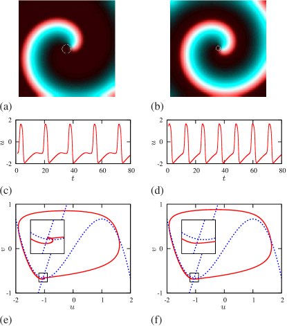
Figure 1: (Color online) A pair of alternative vortices for the same model parameters: $\alpha=0.3,\;\beta=0.72,\;\gamma=0.5$. (Left) slow solution and (right) fast solution. (a,b) spiral waves, shown is the $u$-field, and tip trace; (c,d) action potentials; (e,f) phase portraits, enlarged is the area around the fixed point.

The shaded region in Fig. 2 shows the portion of parameter space, for fixed $\gamma=0.5$, where alternative vortices exist. This region has been computed as part of the present study. Fast spirals exist to the lower left while slow spirals exist to the upper right. Within the cusp-shaped region both types of vortices exist with bistability between them. The boundaries of the bistable region are fold singularies (limit points) meeting at a cusp, $(\alpha,\beta)\approx(0.27,0.8)$. Above the cusp, fast and slow vortices are connected continuously. The thin vertical line shows a representative one-parameter cut, $\alpha=0.3$, that will be the focus of much of our study. The dashed line relates to a 3D phenomenon which we now address.

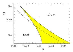
Figure 2: (Color online) Portion of the parameter space of the FitzHugh-Nagumo model containing alternative vortices. $\gamma$ is fixed at $0.5$. Within the shaded cusp-shapped region both fast and slow vortices exist. The thin vertical line at $\alpha=0.3$ shows the parameter cut considered throughout the paper. The dashed curve marks a line of zero filament tension. To the lower left of this curve fast vortices have positive filament tension.

In 3D, scroll waves are organized about filaments and the possible behavior is richer than in 2D. Filaments are not, in general, fixed in space but instead undergo motion, typically on a slow timescale relative to the rotation period. Hence, in addition to whatever dynamics 2D spiral waves might have, scroll waves exhibit additional dynamics associated with filament motion Yakushevich-1984 ; Panfilov-Pertsov-1984 ; Panfilov-etal-1986 ; Panfilov-Rudenko-1987 . Working in Frenet coordinates, the motion may be conveniently expressed in terms of the velocities $V_{N}$ and $V_{B}$ in the normal and binormal directions, respectively, at each point along the filament. Motion along the tangential direction is of no physical significance and is equivalent to reparametrization of the filament.

First semi-phenomenologically Brazhnik-etal-1987 and later using asymptotics Keener-1988 ; Biktashev-1989 ; Biktashev-etal-1994 , the equations of filament motion have been obtained. At lowest order these are

$$V_{N}=b_{2}\kappa+\dots,\qquad V_{B}=c_{3}\kappa+\dots,$$ (3)

where $\kappa$ is the filament curvature. The coefficients $b_{2}$ and $c_{3}$ depend on properties of the medium and 2D spiral solutions. The coefficient $b_{2}$ is called the filament tension. To understand this, consider a circular filament, i.e. a scroll ring. For positive $b_{2}$ a scroll ring will contract somewhat as if the ring were an elastic ring under tension. For negative $b_{2}$, the ring will expand, as though under negative tension. More generally in the negative-tension case, filaments will increase in length and eventually evolve into full scale autowave turbulence Biktashev-1998 . The dashed curve in Fig. 2 indicates a change of sign of filament tension discussed at length later in the paper. The coefficient $c_{3}$, which we shall call the binormal drift coefficient describes the drift of a scroll ring perpendicular to the plane of the ring, or more generally, the velocity component orthogonal to the local plane of the filament.

The remainder of the paper is then devoted to understanding the alternative vortices in 2D and 3D. We first consider relevant asymptotic theory and discuss how Response Functions can be used to predict the filament tension of the alternative vortices. We then investigate the dynamics of the alternative vortices in 2D and 3D through direct numerical simulations. In addition to confirming the prediction, we study how the alternative vortices can be converted one into another in a variety of situations.

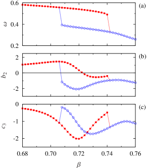
Figure 3: (Color online) Alternative vortices along the parameter cut $\alpha=0.30,\>\gamma=0.5$ shown in Fig. 2. Red squares are fast spirals and blue circle are slow spirals. (a) Hysteresis loop in the rotation velocity $\omega$. (b) Prediction for filament tension $b_{2}$. (c) Prediction for the binormal drift coefficient $c_{3}$.

II Asymptotical Predictions

II.1 Filament tension and drift

At leading asymptotic order, the motion of scroll filaments is determined by the two coefficients $b_{2}$ and $c_{3}$ appearing in Eqs. (3). Once these coefficients are known, the most important properties of filament dynamics, especially the sign of the coefficient $b_{2}$ determining the sign of the filament tension, are determined.

The coefficients for filament motion in Eqs. (3) are given by the following simple formula Biktashev-1989 ; Biktashev-etal-1994

$$b_{2}+ic_{3}=\left\langle\mathbf{W}^{(1)}\,,\,\mathbf{D}\mathbf{V}^{(1)}\right\rangle,$$ (4)

where angle brackets denote an inner product, $\mathbf{V}^{(1)}$ is a Goldstone mode, $\mathbf{W}^{(1)}$ is the corresponding Response Function (RF), and $\mathbf{D}$ is a diffusion matrix. We now elaborate, although we refer the reader to other publications for most technical details Keener-1988 ; Biktashev-etal-1994 ; Biktashev-Holden-1995 ; Biktasheva-Biktashev-2003 ; Biktasheva-etal-2010 .

First consider a rotating spiral wave solution of Eqs. (1)-(2). It is convenient to work in a frame of reference co-rotating with the spiral, at angular velocity $\omega$. Denote the steady spiral seen in this co-rotating frame by $\mathbf{U}=(u,v)^{\mathrm{T}}$.

Now consider the linear stability of such a spiral. Due to symmetries of the system, there will be three eigenvalues given by $\lambda=in\omega$, with corresponding eigenvectors or Goldstone modes $\mathbf{V}^{(n)}$, where $n=-1,0,1$. The $n=0$ eigenvalue and Goldstone mode is related to rotational symmetry and the complex pair of eigenvalues and Goldstone modes $n=\pm 1$ is related to translational symmetry.

In addition to the linear stability problem there is the associated adjoint problem. The adjoints eigenmodes corresponding to eigenvalues $-in\omega$ are the RFs and are denoted $\mathbf{W}^{(n)}$. Thus one sees that to obtain the coefficients for filament motion in Eq. (4) we require the translational Goldstone mode $\mathbf{V}^{(1)}$ and corresponding Response Function $\mathbf{W}^{(1)}$. $\mathbf{D}$ is just the matrix of diffusion coefficients appearing in the reaction-diffusion equations, so for Eqs. (1)-(2), $\mathbf{D}=\left[\begin{array}[]{cccccccc}1&0\\ 0&0\end{array}\right]$. The angle brackets in Eq. (4) signify a straightforward integration over space of the Hermitian product of the vector fields. We note that similar methods employing RFs can be used to obtain the drift velocities of vortices in response to perturbations to Eqs. (1)-(2) Biktasheva-etal-1999 ; Biktasheva-2000 ; Henry-Hakim-2002 ; Biktasheva-etal-2010 .

The prediction of filament tension, and more generally drift velocities, relies on two conditions: firstly, the localization of the RFs $\mathbf{W}^{(n)}$ in the vicinity of the core of the spiral and secondly, the ability to compute the RFs efficiently and accurately. Existence of localized RFs has been demonstrated for a broad range of the models’ parameters in several models Hamm-1997 ; Biktasheva-etal-1998 ; Biktasheva-Biktashev-2001 ; Henry-Hakim-2002 ; Biktasheva-etal-2006 ; Biktasheva-etal-2009 ; Biktashev-etal-2010a . A robust method to compute the RFs with good accuracy for any model of excitable medium with differentiable kinetics has been developed in Ref. Biktasheva-etal-2009, , extending eariler stability methods Wheeler-Barkley-2006 . Using these methods, we have computed the steady spiral $\mathbf{U}$, its rotational velocity $\omega$ together with the Goldstone modes $\mathbf{V}^{(n)}$ and the response functions $\mathbf{W}^{(n)}$ for model (1)-(2) on a disk of radius $\rho_{\max}=25$ with $N_{\theta}=64$ grid points in the angular direction and $N_{\rho}=251$ grid points in the radial direction, see Fig. 4.

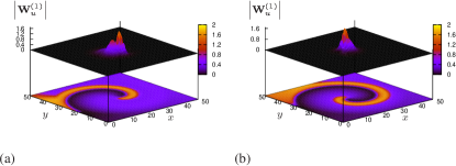
Figure 4: (color online) Spiral waves, shown is the $u$-field (below, flat), and their translational response functions $\left|\mathbf{W}^{(1)}_{u}\right|$ (above, elevated surface) for (a) the slow solution, and (b) the fast solution; $\beta=0.72$.

We focus now on the parameter path indicated in Fig. 2. For $\alpha=0.3$ and $\gamma=0.5$ the hysteresis loop in the spirals’ rotational velocity $\omega$ has been obtained by continuation in parameter $\beta$. As is seen in Fig. 3(a), for these parameters, alternative stable spiral wave solutions with distinct $\omega$ exist in the range $\beta_{\ell}\leq\beta\leq\beta_{u}$, where $\beta_{\ell}\approx 0.708$, $\beta_{u}\approx 0.740$.

We have also computed the filament tension $b_{2}$ and the drift coefficient $c_{3}$ along this parameter path and the results are shown in Figs. 3(b) and 3(c). The most significant feature of these results is the sign change of the filament tension within the hysteresis loop. Below $\beta=\beta_{*}\approx 0.722$, the alternative vortices have filament tension of opposite signs: the fast vortex has positive tension while the slow one has negative tension. At $\beta=\beta_{*}$, the filament tension of the fast vortex changes sign so that in the parameter range $\beta_{*}\leq\beta\leq\beta_{u}$, the alternative vortices both have negative filament tension.

The drift coefficient $c_{3}$ computed in this parameter cut is of fixed sign (negative). The graphs of this drift coefficient of the alternative vortices cross at $\beta\approx 0.726$.

II.2 Scroll rings and electrophoretic drift

There is a connection between filament motion of scroll rings and the drift of spiral waves in response to applied electric fields (electrophoretic drift). Both things will appear in the subsequent numerical studies and it is appropriate to summarize the issues here.

A scroll ring not only has a circular filament, but the entire solution has an axial symmetry. It is convenient to study such a structure in cylindrical coordinates $(r,\theta,z)$, where by symmetry, the solution is independent of $\theta$. Hence the diffusion term in Eq. (1) becomes

$$\nabla^{2}u(r,z)=\left(\frac{\partial^{2}}{\partial r^{2}}+\frac{1}{r}\frac{\partial}{\partial r}+\frac{\partial^{2}}{\partial z^{2}}\right)u(r,z).$$

In this way scroll rings may be studied using 2D numerical computations as long as one is not interested in any symmetry-breaking effects. Moreover, if one is interested in scroll rings with small curvature $\kappa$, corresponding to rings of large filament radius $R=1/\kappa$, one may use the approximation

$$\nabla^{2}u(r,z)\approx\left(\frac{\partial^{2}}{\partial r^{2}}+\kappa\frac{\partial}{\partial r}+\frac{\partial^{2}}{\partial z^{2}}\right)u(r,z),$$ (5)

For small-curvature rings this is an exceedingly accurate approximation. In fact it is equivalent to considering only the lowest-order curvature contributions as in Eqs. (3). We shall use this approach to evaluate filament tension and drift. Note that the normal to the scroll ring points in the outward radial direction and so a positive normal velocity $V_{N}>0$ corresponds to decreasing $r$, and vice versa.

Returning to the 2D Cartesian situation, if the excitable medium is a reaction-diffusion system in which the $u$ reagent is electrically charged and the $v$ is neutral, then the effect of applying an electric field can be modeled by including a term

$$\mathcal{E}\frac{\partial{u}}{\partial{x}},$$ (6)

on the right hand side of Eq. (1), where $\mathcal{E}$ is proportional to the applied electric field which is taken to be in the $x$ direction.

For small values of $\mathcal{E}$, the effect of such a term will be drift of the spiral and one can calculate, using Response Functions, the drift velocity Henry-Hakim-2002 ; Biktasheva-etal-2010 . However, one can use the formal equivalence Panfilov-etal-1986 between the term $\mathcal{E}\partial{u}/\partial{x}$ of Eq. (6) and the term $\kappa\partial{u}/\partial r$ in Eq. (5) to obtain the drift velocity for vortex rings from the results for the applied electric field. Note, that electrophoretic drift towards negative $x$ corresponds to positive filament tension and towards positive $x$ corresponds to negative filament tension.

III Two-Dimensional Simulations

2D simulations have been performed with a suitably modified version of EZSPIRAL Barkley-1991 ; ezspiral . Unless specified otherwise, simulations have been performed using forward Euler timestepping on a uniform Cartesian grid on square domains $40\times 40\>$s.u. with non-flux boundary conditions, nine-point approximation of the Laplacian, spatial discretization $\Delta x=\Delta y=h=1/3$ and time step $\Delta t=3/80$. The tip of the spiral is defined as the intersections of isolines $u(x,y)=u_{*}$ and $v(x,y)=v_{*}$, and the angle between $\nabla u$ at the tip and $x$ axis is taken as orientation of the tip. We use $(u_{*},v_{*})=(0,0)$ for the FitzHugh-Nagumo model. Initial conditions for the alternative spirals have been computed using parameter continuation and then converted into the input format of EZSPIRAL.

III.1 Alternative vortices: conversion by a shock

First, to test if the alternative vortices can be converted from one into another in a controllable way, we add a constant value $A$ to the fast variable $u$, uniformily in space, at a specified time instant $T$.

$$u(x,y,t)\rightarrow u(x,y,t)+A,\quad\mbox{at $t=T$}$$ (7)

This may be considered as a very crude model of a defibrillating shock. We use a box size of $50\times 50\>$s.u., and in selected simulations up to $150\times 150\>$s.u., with spatial discretization $h=0.1$ and time step $\Delta t=2.25\times 10^{-3}$.

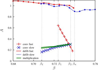
Figure 5: (Color online) Minimum shock amplitudes $A$ needed to convert one type of spiral into the other (lines with large symbols), in comparison with the corresponding defibrillation thresholds (dashed and dotted lines). In the legend, ’conv fast’/’conv slow’ refers to the shocks applied to fast/slow spirals necessary for conversion. Likewise, ’defib fast’/’defib slow’ refers to the shocks applied to fast/slow spirals necessary for defibrillation. The thick solid lines above the ’conv slow’ curve indicate the region of parameters causing conversion with multiplication via front break-up.

The minimum shock amplitudes required to convert one alternative vortex into another are shown in Fig. 5, together with the corresponding “defibrillation thresholds” that are sufficient for the complete elimination of spiral-wave activity.

It can be seen that, within the parameter range of the hysteresis $\beta_{\ell}\leq\beta\leq\beta_{u}$, there are three distinct intervals of behavior demarked by the values $\beta_{1}\approx 0.722$ and $\beta_{2}\approx 0.736$. In the region between $\beta_{\ell}$ and $\beta_{1}$ it is possible to convert a slow vortex into its faster counterpart. Transitions in the opposite direction have not been observed, even as we increase $A$ to the defibrillation threshold, which eliminates spirals from the medium. In the middle interval, between $\beta_{1}$ and $\beta_{2}$, conversion both ways is possible. For $\beta$ in the range between $\beta_{2}$ and $\beta_{u}$, we only observe conversions from fast vortices into their slow counterparts, but not vice versa.

The value of $\beta_{1}$, which is the smallest $\beta$ for which conversion is possible from fast to slow vortices with a single shock, is close to $\beta_{*}$ at which the filament tension of the fast vortices is zero. This is a purely empirical observation and we have not investigated how precisely it holds.

We also observed conversion with multiplication from a slow vortex with a large core into multiple fast vortices with small cores, via break-up of some segments of excitation fronts. This is illustrated in Fig. 6. This conversion with multiplication occurs in a very small range of shock amplitudes just above the conversion amplitude; the numerical values are listed in Table 1. Note that break-up of spiral waves by spatially uniform shocks has been previously observed, e.g. Ref. Keener-Panfilov-1996, , in cases without bistability, but at shock magnitudes close to the defibrillation threshold. Here we observe it in a system with alternative spiral waves, at shock magnitudes significantly smaller than the defibrillation threshold and only slightly above the conversion threshold. We have not observed conversion with multiplication from a fast spiral into multiple slow spirals by any shock amplitude.

Figure 6: (Color online) Shock conversion with multiplication at $\beta=0.73$. (a) Slow vortex with the large core before the shock. (b) Front breaks immediately after a shock of amplitude $A=0.29$. (c) Multiple fast spirals with small cores, approximately $50.3$ t.u. after the shock.

$\beta$	$A_{\min}$	$A_{\max}$
0.70735	0.2306	0.2452
0.710	0.2357	0.2511
0.715	0.2463	0.2602
0.720	0.2552	0.2642
0.724	0.2625	0.2805
0.725	0.2628	0.2834
0.726	0.2657	0.2850
0.728	0.2730	0.2896
0.730	0.2813	0.2946
0.730	0.2818	0.2941
0.732	0.2895	0.2986
0.734	0.2965	0.3032
0.735	0.2991	0.3059
0.736	0.3027	0.3077

Table 1: The minimum $A_{\min}$ and maximum $A_{\max}$ shock amplitudes producing multiple spirals from a slow vortex.

III.2 Conversion due to interaction with the boundary

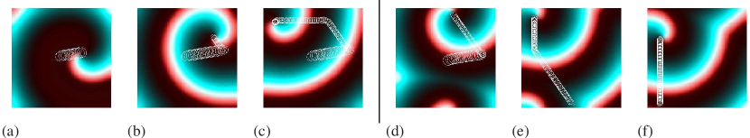
Figure 7: (Color online) Conversion due to do interaction with a boundary. Simulations are started with a slow spiral at $\beta=0.71$. The spiral is induced to drift toward the right boundary by electrophoresis perturbation of amplitude $\mathcal{E}=0.03$. (a-c) Three snapshots of the evolution with Neumann boundaries conditions on all four sides. (d-f) Three snapshots of the evolution with Neumann boundaries conditions on right and left, and periodic boundary conditions on top and bottom.

To study how interaction with a boundary may bring about conversion, we gently push the spiral towards a boundary using electrophoretic drift discussed in Sec. II.2. Recall that negative tension ($b_{2}<0$) corresponds to electrophoretic drift to the right and positive tension ($b_{2}>0$) corresponds to drift to the left.

Representative simulations are shown in Fig. 7 at $\beta=0.71$. Simulations are started from the slow, large-core spiral. The period of the spiral is $T\approx 16.8654$. The spiral drifts from its initial position to the right in agreement with the predicted negative filament tension, $b_{2}<0$. It also moves up, as it should, since predicted drift coefficient, $c_{3}$ is negative. When the spiral nears a boundary, its core radius decreases significantly and its period changes to $T\approx 11.2964$. The horizontal drift component changes sign [Fig. 7(b)], corresponding to switching to positive filament tension, and the spiral moves to the left rather than to the right. The binormal component of drift changes magnitude but not sign.

At the top boundary, the spiral drifts to the left until it pins to the top left corner of the box [Fig. 7(c)]. If the Neumann boundary conditions (NBCs) at the top and bottom edges of the box are changed to periodic boundary conditions (PBCs), the fast spiral with a small core will continue to drift upwards along the left boundary indefinitely [Fig. 7(d-f)].

III.3 Conversion due to applied field

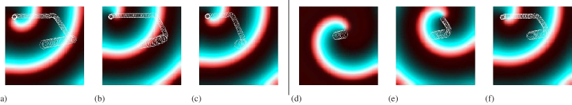
Figure 8: (Color online) Conversion due to allied fields. All simulations start from a slow spiral at $\beta=0.71$. (a-c) Three simulations for field strengths (a) $\mathcal{E}=0.035$, (b) $\mathcal{E}=0.0472$, (c) $\mathcal{E}=0.06$. In (a) conversion occurs at the boundary, whereas for (b,c) conversion occurs due to sufficiently strong electrophoretic drift. (d-f) Three snapshots of a single simulation with $\mathcal{E}=0.03$. After 8 rotations a shock of strength $A=0.14889$ is applied resulting in conversion.

Electrophoretic driving of a sufficiently high magnitude can itself cause conversion of vortices directly. Figure 8 shows selected simulations illustrating this phenomenon. Figure 8(a) shows that $\mathcal{E}=0.035$ is not strong enough to convert the slow spiral into the fast, and indeed it allows the spiral to continue to drift to the right boundary, at which the conversion happens. Figure 8(b) shows the simulation with the threshold amplitude $\mathcal{E}=0.0472$, allowing the conversion to happen well before reaching the boundary. Finally, Fig. 8(c) shows a simulation with $\mathcal{E}=0.06$ which is strong enough to convert the slow spiral into the fast one almost immediately.

Figures 8(d-f) illustrate the combined effect of an electrophoretic driving and defibrillation-style shock. Shocks of various amplitudes are applied after 8 rotation periods of the slow spiral. If the amplitude is sufficiently high, conversion happens before the spiral reaches the boundary. In the presence of electrophoretic driving with $\mathcal{E}=0.03$, we find that the minimal shock strength required for conversion is $A_{\mathrm{conv}}\approx 0.1489$ (the case shown in the figure), which is slightly smaller than that $A_{\mathrm{conv}}\approx 0.1789$ required for conversion in the absence of applied field ($\mathcal{E}=0$).

III.4 Verfication of predictions and effects of discretization

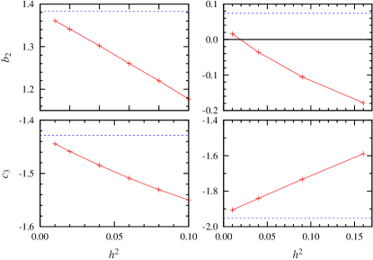
Figure 9: (Color online) Numerical convergence of $b_{2}$ and $c_{3}$ from numerical simulations of electrophoretic drift. The fast vortex is simulated over regular grid spacings $\Delta r=\Delta z=h$ as indicated. Left column: $\beta=0.71$, a typical case away from $b_{2}=0$. Both coefficients converge quadratically in $h$ to the values predicted by RFs (blue dashed lines). Right column: $\beta=0.722$, a case close to $b_{2}=0$ where filament tension is small. $c_{3}$ converges quadratically while the convergence of $b_{2}$ is less clear. Importantly, except at very high resolution the tension in the simulation is of the opposite sign from the asymptotic result.

Before proceeding to 3D simulations, we compared the predictions for the filament tension $b_{2}$ and binormal drift coefficient $c_{3}$ obtained via RFs in Sec. II, with direct 2D computer simulations of axisymmetric scroll rings as discussed in Sec. II.2. From the motion of the axisymmetric filament in the radial (normal) and vertical (binormal) directions we obtain the coefficients $b_{2}$ and $c_{3}$. In 2D, it is possible to perform simulations to very high spatial resolution with reasonable cost and hence we are also able to study systematically the effects of numerical resolution.

Simulations of electrophoretic drift at $\mathcal{E}=0.01$ have been conducted for the fast vortex over a variety of regular grids with spacings $\Delta r=\Delta z=h$. Results are shown in Fig. 9 for two values of $\beta$: $\beta=0.71$, a typical case away from where $b_{2}$ crosses zero in Fig. 3, and $\beta=0.722$, a case very near the zero crossing of $b_{2}$. In the typical case, left column of Fig. 9, both $b_{2}$ and $c_{3}$ converge extremely well as the grid size goes to zero to the predicted values given by Eq. (4). The convergence is quadratic, i.e. linear in $h^{2}$, as is consistent with the second-order accuracy of the numerical simulation.

The case shown in the right column of Fig. 9, where the predicted value of $b_{2}$ is small, is more problematic. Again, $c_{3}$ converge extremely well, and with the expected form, to the predicted result. The convergence of the tension $b_{2}$ is less satisfying, both in the form of the convergence and in the asymptotic value. The exact reasons for this are outside the focus of the current study. The important point is the sign change of $b_{2}$ seen in the right column of Fig. 9 due to finite resolution. This means that a 3D numerical simulation performed at even high resolution, e.g. $h=0.2$ will be qualitatively different from a fully resolved simulation at these parameter values, since the simulated filament tension will be negative whereas the fully resolved tension is positive.

The conclusion is that the filament tension and binormal drift predicted from RFs and plotted in Fig. 3 are borne out by direct numerical simulations. Nevertheless, 3D simulations should only be performed for the model parameters such that the discretization does not qualitatively affect the simulations by artificially changing the sign of the filament tension. For the parameters we consider, this means to the left ($\beta\leq 0.71$) or the right ($\beta\geq 0.73$) sides of zero crossing of $b_{2}$ in Fig. 3.

IV Three-dimensional simulations

We have seen in Sec. III that it is possible convert between fast and slow vortices in 2D by a variety of mechanisms, such as interactions with boundaries and shocks. These effects will also exist in 3D, but in 3D the additional effects arising due to filament curvature and filament tension can be hugely important. This is especially so in the region where, according to predictions of Sec. II, the alternative vortices have opposite signs of filament tension.

Simulations have been performed with a version of EZSCROLL Dowle-etal-1997 ; ezscroll modified for FHN kinetics. The simulations use forward Euler timestepping on a uniform Cartesian grid on cuboid domains of varying size with non-flux boundary conditions, nineteen-point approximation of the Laplacian, space discretization step $\Delta x=\Delta y=\Delta z=h=1/3$ and time discretiation step $\Delta t=3/80$. Numerical determination of the instant position of scroll filaments is technically challenging, and we use an easy substitute: the instant phase singularity lines, defined as the intersections of isolines $u(x,y)=u_{*}$ and $v(x,y)=v_{*}$. Such singularity lines correspond to spiral tips in 2D, and like a spiral tip rotates around the current rotation center, so a singularity line rotates around the current filament. We also assume that inasmuch as the twist of scroll waves is insignificant, then the curvature of the singularity line is close to the curvature of the filament, so we take the former as an approximation of the latter. As with 2D simulations in EZSPIRAL, we use $(u_{*},v_{*})=(0,0)$ for the FitzHugh-Nagumo model, with some exceptions, described later. Initial conditions for alternative scrolls are obtained by first computing alternative spirals on a polar grid, using methods described in Ref. Biktasheva-etal-2009, , then converting these solutions to Cartesian coordinates and “stacking” spirals on top of one other to generate 3D scroll waves.

It is more difficult in 3D than in 2D to use core size and visual inspection to distinguish between fast and slow vortices. However, point records of the action potentials, $u(t)$ at some fixed location, may clearly distinguish the two types of vortices. Recall Fig. 1. Slow vortices have extra maxima in the tails of their action potentials, the DADs, while fast vortices do not, no DADs. This method of distinguishing between vortices assumes that the whole solution consists of only slow or only fast vortices. A more sophisticated method free from this assumption is described later.

IV.1 Alternative vortices with opposite signs of filament tension

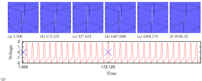
Figure 10: (Color online) Evolution of a fast helical scroll with positive filament tension at $\beta=0.71$. The domain has Neumann boundary conditions. (a-f) The filament straightens up (the numbers under the snapshots show corresponding time in timeunits); (g) action potentials with blue crosses marking the times at which two of the snapshots are taken. Singularity lines are used as approximations to the scroll filament.

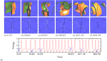
Figure 11: (Color online) Evolution of a slow helical scroll with negative filament tension at $\beta=0.71$. Same domain and parameters as for the fast vortex in Fig. 10. (a-f) (Top) isosurfaces of the $u$-field; (middle) filament only (as in Fig. 10). (g) action potentials with blue crosses marking the times at which the snapshots are taken. The helix initially expands as expected for negative tension, but then undergoes conversion and contracts.

The first case we consider is at $\beta=0.71$, where the fast and slow vortices have opposite signs of filament tension. Simulations have been conducted in a box of size $50\times 50\times 50$ s.u., with Neumann boundary conditions (NBCs) on all sides. Simulations are started from alternative vortices with filaments in the form of helices constructed by layering 2D solutions such as to create a helical scroll with one turn from bottom to top. The radius of the helix is 2 s.u. We expect that the filament of the fast vortex with positive filament tension will straighten up while slow vortex with negative filament tension will expand, possibly breaking up and developing into turbulence.

Figure 10 shows the evolution of the fast vortex with positive filament tension. As expected, the filament straightens up, see Fig. 10(a-f). The record of corresponding action potential, Fig. 10(g), shows that there is no conversion into the slow alternative vortex: no DADs appeared.

Figure 11 shows the evolution of the slow vortex with negative filament tension. First, the filament expands as expected. However, after five full rotations, the vortex spontaneously changes its period and converts into its fast counterpart with positive filament tension, and we see DADs disappearing at this moment in Fig. 11(g). The fast, positive filament tension vortex subsequently contracts, see Fig. 11(d-f), and disappears.

IV.2 Conversion due to curvature

To identify the cause for the spontaneous conversion in the simulations just discussed, we have repeated the simulation with the slow helical vortex in different domain sizes with periodic boundary conditions (PBCs) on the top and bottom of the domain, and NBCs elsewhere.

In this series of simulations, we start from a helical filament with one full turn from bottom to top. We monitor the mean radius of the projected filament onto the base of the box. Initially the projection is a circle. The initial helical filament expands. As this expansion is inherently unstable, the projections of the filament onto the base very soon cease to be circular. See Figs. 12-14.

Figure 15(a) shows how the mean radius of a vortex filament’s projection changes every period in the boxes $50\times 50\times 50$ s.u., $50\times 50\times 100$ s.u. and $70\times 70\times 50$ s.u. The vertical lines show the time at which conversion happens in each box, as indicated by the morphology of the point records. It can be seen that in the boxes $50\times 50\times 50$ s.u. and $70\times 70\times 50$ s.u., both of height $L_{z}=50$ s.u., conversion happens at approximately the same time, regardless of the width of the box. Whereas in the box $50\times 50\times 100$ s.u. with the height $100$s.u. conversion happens much later than in the other two cases. Comparing the simulations in boxes $50\times 50\times 50$ s.u. and $50\times 50\times 100$ s.u., one can conclude that interaction with the boundary is probably not the main factor in the conversion, as it takes significantly different times in the boxes of the same width, and similar times in boxes of different widths.

Critical curvature is a more plausible cause for conversion. On qualitative level, larger $L_{z}$ means smaller initial curvature and, by Eq. (3), slower evolution. This is indeed what happens: the helix with $L_{z}=100$ expands more slowly than those with $L_{z}=50$. See Fig. 15(a). Thus it will take longer for the filament curvature to reach any particular value, e.g. its critical value.

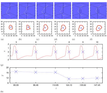
Figure 12: (Color online) Conversion of a slow helical vortex into a fast one at $\beta=0.71$. Domain size is $50\times 50\times 50$ s.u. with PBC on top and bottom and NBC elsewhere. (a-f) evolution of the filament (top row) and projections of the filament onto the base of the box (second row) shown in red, with the barycenter shown as a blue cross and the mean radius shown as the green circle. (g) action potentials ($u$-field against time $t$), blue crosses correspond to the times at which the snapshots in (a-f) are taken, and the period number is shown on the upper axis. (h) period $T$ plotted against time $t$.

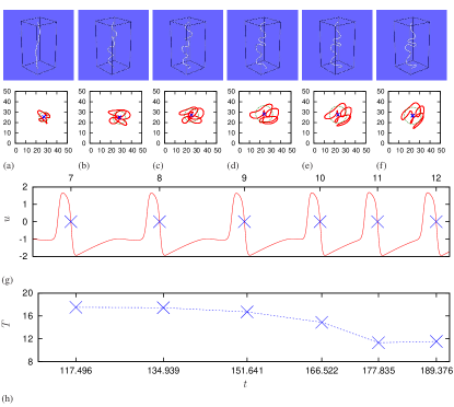
Figure 13: (Color online) Same as in Fig. 12 except with a box of size $50\times 50\times 100$ s.u.

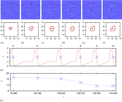
Figure 14: (Color online) Same as in Fig. 12 except with a box of size $70\times 70\times 50$ s.u.

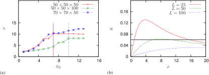
Figure 15: (Color online) Curvature evolution. (a) The mean radius, $\rho$, of the $(x,y)$ projection of the filament, against the period number, $N_{T}$. The vertical lines separate the slow region (to the left of the line) from the fast region (to the right). (b) Dependence of the curvature, $\kappa$, on the radius of the projection, $\rho$, using Eq. (8) for an ideal helix. The horizontal line is the critical curvature, $\kappa_{\mathrm{crit}}$.

To quantify this argument, consider an ideal helix whose curvature $\kappa$ depends on the radius of its projection $\rho$ as

$$\kappa=\frac{\rho}{\rho^{2}+\left(L_{z}/2\pi\right)^{2}}\,,$$ (8)

where $L_{z}$ is the height of the helix making one full turn. Figure 15(b) shows how the curvature $\kappa$ of an ideal helix changes with $\rho$, for the selected values of $L_{z}$. The important feature is that the curvature of a helix increases with $\rho$ up to a certain maximum which depends on $L_{z}$. The larger $L_{z}$, the slower the growth of $\kappa$ with $\rho$ and the smaller the maximum. For comparison, we also show on Fig. 15(b) the curvature $\kappa_{\mathrm{crit}}$, which causes immediate conversion. This is known from the 2D simulation shown in Fig. 8(c) where $\mathcal{E}=0.06$ causes immediate conversion. Again using the formal equivalence between electrophoresis and curvature (Sec. II.2), we have $\kappa_{\mathrm{crit}}=0.06$.

These graphs imply that for an ideal vortex, the conversion due to curvature will happen later for larger $L_{z}$, which is in qualitative agreement with the observations shown in Fig. 15(a). However, there is no quantitative agreement. This is likely because the shape of the filaments very soon deviates from an ideal helix.

We have explicitly calculated the curvature of the filaments using numerical differentiation with Tikhonov regularization. The details of the procedure can be found in Appendix A. The results of this analysis are presented in Fig. 16(a) and Fig. 17(a), with the local curvature shown against $z$ coordinate on the filament, for selected values of the scroll period numbers $N_{T}$. We see that the curvature grows very non-uniformly, both along the filament and in time.

To detect the conversion visually, so as to be more precise about time and location of the conversion, we have analyzed the fine structure of the scroll cores, using a modified version of the instant phase singularities: $u_{*}=-1.04$, $v_{*}=-0.656$. The idea is that the point $(u_{*},v_{*})$ is within the small loop of the phase trajectory shown in Fig. 1(c), and existence of such a loop is the signature of slow scrolls. Using this definition, slow scrolls are characterized by a double singularity line, whereas the fast scrolls have a single singularity line. See Fig. 16(b-d) and Fig. 17(b-d). One can see that the conversion is indicated by the departing of the secondary singularity from the main one following the period in which the filament curvature (obtained for the standard, “robust” singularity $u_{*}=v_{*}=0$) has exceeded threshold on a substantial continuous interval. We see this as a confirmation that curvature of the filament is the likely cause of the conversion in these simulations.

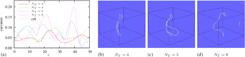
Figure 16: (Color online) Curvature and conversion in the $70\times 70\times 50$ s.u. domain corresponding to the simulation shown in Fig. 14. (a) The curvature against $z$ coordinate on the filament, for selected values of the scroll period numbers $N_{T}$. (b,c,d): the double-singularity visualization of the scrolls (b) immediately before, (c) in the very beginning, and (d) after completion of the conversion.

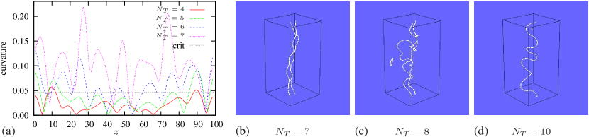
Figure 17: (Color online) Same as in Fig. 16, except for the $50\times 50\times 50$ s.u. simulation shown in Fig. 13.

IV.3 Dynamics of alternative ring vortices

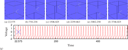
Figure 18: (Color online) Evolution of a fast scroll ring with positive tension at $\beta=0.71$. One quarter of the ring is simulated in a domain with Neumann boundary conditions on four sides and periodic boundary conditions one the top and bottom. Visualizations and time series are as in previous figures.

We have also considered the dynamics of alternative scroll rings with filament tension of opposite sign at $\beta=0.71$. One expects that, at least initially, a ring with positive tension will drift and contract, while a ring with negative filament tension will drift and expand. We are interested in the long-term dynamics of such rings.

A quarter of a scroll ring with positive filament tension is initiated in a cubical box of size $50\times 50\times 50$ s.u. Two cases have been considered. In one the box has Neumann boundary conditions on all sides (not shown) and in the other the box has Neumann boundary conditions on four sides and periodic boundary conditions on the top and bottom (case shown in Fig. 18). The initial radius of the ring is $\approx 25$ s.u. and meets two adjacent sides at right angles as seen in Fig. 18(a).

The scroll drifted upwards, remaining essentially flat. In the case with Neumann boundary conditions on all sides, the ring approaches the upper boundary where it shrinks and eventually disappears in a top corner of the box. With periodic boundary condition, as seen in Fig. 18, instead of collapsing, the ring drifts upwards continuously and reaches an asymptotic constant radius. In a way, this perpetual movement is similar to what was observed in 2D simulations of electrophoretic drift with periodical boundary conditions, Fig. 7(d-f).

The existence of the stable vortex rings in excitable media was first reported by Winfree Winfree-1994 . The upward component of the ring’s velocity at the chosen set of model parameters is in agreement with the asymptotic theory which gives $c_{3}<0$ for $\beta=0.71$. More importantly, it seems that the positive filament tension, $b_{2}>0$, on its own may be not enough for a ring to collapse. It seems that, in the absence of other perturbations, the positive filament tension shrinks a ring vortex just to a stable minimum radius not equal to zero, while the internal interaction of parts of the vortex prevents it from complete collapse. Note that in simulations of vortex rings with positive filament tension, with both Neumann and periodic boundary conditions, there no conversion of the fast vortex into its slow counterpart has been observed.

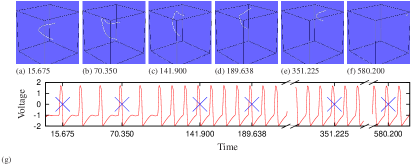
Figure 19: (Color online) Evolution of a slow scroll ring with negative tension at $\beta=0.71$. The simulation is initiate with a quarter of the ring a domain with Neumann boundary conditions on all sides. Visualizations and time series are as in previous figures.

Now consider the evolution of the slow vortex ring with negative filament tension shown in Fig. 19. The model parameters are the same as in the previous simulation although here we show the case with Neumann boundary conditions on all sides of the domain. In accordance with the negative filament tension, the ring initially expands [Fig. 19(a-b)] and becomes non-planar. After five rotations the vortex converts into its fast counterpart (with positive tension), as seen in the action potential recordings in Fig. 19(g). From this point the vortex propagates to the top boundary where it contracts and disappears in the top corner, Fig. 19(c-f).

In case of periodic boundary conditions (not shown) the scenario is: expansion due to negative tension followed by conversion to the fast vortex with positive filament tension, followed by contraction to a stable ring with a nonzero radius, similar to Fig. 18. The same type of scenario was first reported by Sutcliffe and Winfree Sutcliffe-Winfree-2003 who explained it by the twist of the filament. Here we have demonstrated that the switching from expansion to contraction could be due to simple switching from a vortex with negative filament tension to its counterpart with positive filament tension.

IV.4 Alternative vortices with negative filament tension

At $\beta=0.73$, the alternative solutions both have negative filament tension, as can be seen Fig. 3. Still, only the slower vortex displays DADs in its action potentials. As we know from the 2D studies [Fig. 5], at these model parameters conversion is possible both ways, from slow to fast and from fast to slow vortex.

First we consider the evolution of a helical vortex initiated from the fast spiral shown in Fig. 20. Simulations are in a box of size $50\times 50\times 50$ s.u., with Neumann boundary conditions on all sides. The filament initially expands due to negative tension, but quickly converts to the slow scroll after just two rotations. See the DADs appeared in Fig. 20(g). The slower vortex continues to expand and then converts back to the fast vortex after 14 periods. Since both alternative vortices have negative tension, eventually full fibrillation with multiple filaments develops as is seen Fig. 20(c). There are no further spontaneous conversions, and the fast vortex with negative filament tension continues to evolve. However, we see a gradual reduction in the number of filaments until only a single tiny piece persists in the bottom right corner of the box.

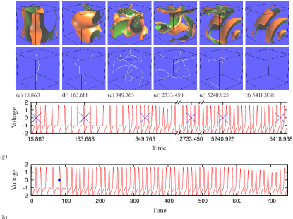
Figure 20: (Color online) Evolution when alternative scrolls both have negative filament tension, $\beta=0.73$. Simulations start with a fast helical scroll. The boundary conditions are Neumann on all boundaries. (a–f) (Top row) isosurfaces of the $u$-field; (second row) filaments only. (g) Action potentials with blue crosses marking the times at which the snapshots are taken. (h) Action potentials for a simulation with the same initial and boundary conditions, but with a shock stimulus applied at the instant marked with a blue dot).

Thus far, we have observed only spontaneous conversion between alternative vortices in 3D. It is important for cardiological applications to verify whether 3D vortices can be converted by a shock. Having the prolonged period of slow vortex evolution in the simulation shown in Fig. 20(g), we have repeated the simulation and this time applying a uniform shock, Eq. (7), to the slow vortex. The action potential time series, but not the visualization, are shown in Fig. 20(h). A shock of amplitude $A=0.8$ is applied just after the third slow vortex period. The shock successfully converts the slow vortex into its fast counterpart. The rest of the evolution of the fast scroll was similar to Fig. 20(a-f): development of the full fibrillation followed by gradual reduction of the number of filaments in the box to just a single tiny persistent piece in the top right corner of the box, but in approximately half of the time taken without the shock.

V Discussion

In this study we have investigated dynamics of alternative spiral and scroll waves in the FitzHugh-Nagumo model, in a parameter region of bistability between distinct alternative vortices. Some of the features have been noted already by Winfree Winfree-1991a who discovered such alternative solutions. Here we have extended those studies and related them to the asymptotic theory of spiral and scroll wave dynamics. The most important features are:

1. There is a parameter region in FHN model where stable alternative spiral wave solutions, with different rotation frequencies, exist. Faster spiral waves have the normal morphology of the “action potential” whereas the slower spiral waves show “delayed after-depolarization” morphology.

2. The alternative vortices can convert one into the other as a result of a variety of perturbations, such as a homogeneous pulse stimulus or interaction with a boundary. There are distinct parametric regions where this transition may occur in one direction only, either from slow to fast vortex or from fast to slow, as well as the regions where the transition can occur in both directions. Conversion of a single slow vortex into multiple fast vortices is also possible.

3. The conversion effects of spirals can also be observed for scroll waves. In addition, scroll waves can demonstrate spontaneous conversion apparently related to the filament curvature.

4. In accordance with the predictions of the asymptotic theory, the alternative scroll waves have significantly different filament tensions. In particular, the filament tension of the faster scroll waves changes sign in the parametric interval considered, whereas the slow scroll waves have negative filament tension in this interval. Therefore, there exists a parameter region where the fast vortex with positive filament tension has a slow counterpart with negative filament tension, and a parameter region where both alternative vortices have negative filament tension. The scrolls with positive filament tension have tendency to contract, or straighten up if the filament connects opposite surfaces of the box. The vortex rings with positive filament tension might have a stable radius not equal to zero, and collapse only due to an additional perturbation, e.g. hitting the boundary perpendicular to the axis of the ring.

The scrolls with negative filament tension have the tendency to lengthen and multiply, which can lead to “scroll wave turbulence”, phenomenologically similar to certain stages of cardiac fibrillation. However, interaction of different scroll filaments with each other and/or with the boundary may lead to the stabilization of the scrolls notwithstanding the effects of the filament tension, as was observed previously (e.g. Ref. Biktashev-1989, p. 139) and in simulations presented here. Therefore, in three dimensional experiments and simulations the stabilized scrolls with negative filament tension may behave identically to the scrolls with the positive filament tension, and the only way to distinguish between them is to compute/measure their response functions.

The conversion processes summarized in points 2 and 3 above are essentially threshold effects and so are not asymptotic in nature. However, there are examples where (non-asymptotic) analytical approaches have been successful in describing threshold phenomena, Idris-Biktashev-2008 . Following the idea of Ref. Idris-Biktashev-2008, , it may be possible to describe conversion of spiral waves in response to external stimuli using center-stable space of the unstable spiral wave solutions, which presumably separates (in the functional space) the stable alternative spirals observed in simulations.

Assuming that the above features are present in other models, including more physiologically realistic ones, one may conjecture the following scenarios, which may be relevant to cardiac electrophysiology.

Shock-induced conversion of fibrillation to tachycardia. Suppose the cardiac tissue fibrillates due to “scroll turbulence” mechanism, underlied by slow scrolls. Such slow scrolls are likely to convert to fast scrolls either due to curvature or to interaction with each other or with boundaries. However this may take a long time. An electric shock which is too weak to instantly defibrillate, may still be enough to convert from slow to fast scrolls. If the fast scrolls have positive filament tension, this may lead to “delayed defibrillation”, when the fibrillation stops via collapse of all scrolls, but only many cycles after the shock, or to “tachycardia” when the fast scrolls would stabilize either by connecting opposite surfaces of the tissue (say transmural filaments) or by attaching to localized inhomogeneities or anatomical features.

If the corresponding fast scrolls have negative filament tension, they might stabilize due to interaction with each other and with the boundary, leading to tachycardia indistinguishable from the one with positive filament tension and without pinning to anatomical obstacles.

Intermittent fibrillation. If both alternative scrolls have negative filament tension and can be converted equally one into another, then a relatively weak external shock applied to the stabilized fast scroll can convert it back into the slow one, which will initiate another, may be prolonged fibrillation period before eventual conversion and stabilization back into tachycardia.

FitzHugh-Nagumo model is admittedly very far from realistic cardiac models. However, delayed after-depolarization is indeed known in electrophysiology, and known to have arrhythmogenic effect Wit-Rosen-1983 ; Wu-etal-2004 . The presence of DADs will add to the period of the vortices, and the tendency of vortices with longer periods to have negative filament tension is universalBrazhnik-etal-1987 and not restricted to the FHN model. The coexistence of vortices with different periods and different filament tensions is key to the effects we have described. Hence we believe that the basic phenomenology involved in our results is not restricted to FHN and may be observed in any excitable media with DADs, and so is likely to be relevant to cardiac electrophysiology. This capacity of DAD is distinct from its well-known role as a mechanism of arrhythmia initiation.

References

- (1) T. Frisch, S. Rica, P. Coullet, and J. M. Gilli, “Spiral waves in liquid crystal,” Phys. Rev. Lett. 72, 1471–1474 (1994).
- (2) B. F. Madore and W. L. Freedman, “Self-organizing structures,” Am. Sci. 75, 252–259 (1987).
- (3) L. S. Schulman and P. E. Seiden, “Percolation and galaxies,” Science 233, 425–431 (1986).
- (4) A. M. Zhabotinsky and A. N. Zaikin, “Spatial phenomena in the auto-oscillatory system,” in Oscillatory processes in biological and chemical systems, edited by E. E. Selkov, A. A. Zhabotinsky, and S. E. Shnol (Nauka, Pushchino, 1971) p. 279.
- (5) S. Jakubith, H. H. Rotermund, W. Engel, A. von Oertzen, and G. Ertl, “Spatiotemporal concentration patterns in a surface reaction — propagating and standing waves, rotating spirals, and turbulence,” Phys. Rev. Lett. 65, 3013–3016 (1990).
- (6) M. A. Allessie, F. I. M. Bonke, and F. J. G. Schopman, “Circus movement in rabbit atrial muscle as a mechanism of tachycardia,” Circ. Res. 33, 54–62 (1973).
- (7) N. A. Gorelova and J. Bures, “Spiral waves of spreading depression in the isolated chicken retina,” J. Neurobiol. 14, 353–363 (1983).
- (8) F. Alcantara and M. Monk, “Signal propagation during aggregation in the slime mold Dictyostelium Discoideum,” J. Gen. Microbiol. 85, 321–334 (1974).
- (9) J. Lechleiter, S. Girard, E. Peralta, and D. Clapham, “Spiral calcium wave propagation and annihilation in Xenopus Laevis oocytes,” Science 252 (1991).
- (10) A. B. Carey, R. H. Giles, Jr., and R. G. Mclean, “The landscape epidemiology of rabies in virginia,” Am. J. Trop. Med. Hyg. 27, 573–580 (1978).
- (11) J. D. Murray, E. A. Stanley, and D. L. Brown, “On the spatial spread of rabies among foxes,” Proc. Roy. Soc. Lond. ser. B 229, 111–150 (1986).
- (12) A. G. Shagalov, “Spiral patterns in magnets,” Phys. Lett. A 235, 643–646 (1997).
- (13) P. Oswald and A. Dequidt, “Termomechanically driven spirals in a cholesteric liquid crystals,” Phys. Rev. E 77, 051706 (2008).
- (14) Y. Larionova, O. Egorov, E. Cabrera-Granado, and A. Esteban-Martin, “Intensity spiral patterns in a semiconductor microresonator,” Phys. Rev. A 72, 033825 (2005).
- (15) D. J. Yu, W. P. Lu, and R. G. Harrison, “Dynamic bistability and spiral waves in a laser,” Journal of Optics B — Quantum and Semiclassical Optics 1, 25–30 (1999).
- (16) K. Agladze and O. Steinbock, “Waves and vortices of rust on the surface of corroding steel,” J. Phys. Chem. A 104, 9816–9819 (2000).
- (17) T. Bretschneider, K. Anderson, M. Ecke, A. Müller-Taubenberger, B. Schroth-Diez, H. C. Ishikawa-Ankerhold, and G. Gerisch, “The three-dimensional dynamics of actin waves, a model of cytoskeletal self-organization,” Biophys. J. 96, 2888–2900 (2009).
- (18) M. A. Dahlem and S. C. Müller, “Migraine aura dynamics after reverse retinotopic mapping of weak excitation waves in the primary visual cortex,” Biological Cybernetics 88, 419–424 (2003).
- (19) O. A. Igoshin, R. Welch, D. Kaiser, and G. Oster, “Waves and aggregation patterns in myxobacteria,” Proc. Nat. Acad. Sci. USA 101, 4256–4261 (2004).
- (20) A. T. Winfree, “Alternative stable rotors in an excitable medium,” Physica D 49, 125–140 (1991).
- (21) J. Wu, J. Wu, and D. P. Zipes, “Mechanisms of initiation of ventricular tachyarrhythmias,” in Cardiac Electrophysiology: from Cell to Bedside, Fourth edition, edited by D. P. Zipes and J. Jalife (Saunders, Philadelphia, 2004) pp. 380–389.
- (22) L. Yakushevich, “Vortex filament elasticity in active medium,” Studia Biophysica 100, 195–200 (1984).
- (23) A. V. Panfilov and A. M. Pertsov, “Vortex ring in 3-dimensional active medium described by reaction-diffusion equations,” Doklady Akademii Nauk SSSR 274, 1500–1503 (1984).
- (24) A. V. Panfilov, A. N. Rudenko, and V. I. Krinsky, “Turbulent rings in 3-dimensional active media with diffusion by 2 components,” Biofizika 31, 850–854 (1986).
- (25) A. V. Panfilov and A. N. Rudenko, “Two regimes in scroll ring drift in the three-dimensional active media,” Physica D 28, 215–218 (1987).
- (26) P. K. Brazhnik, V. A. Davydov, V. S. Zykov, and A. S. Mikhailov, “Vortex rings in excitable media,” Sov. Phys. JETP 66, 984–990 (1987).
- (27) J. P. Keener, “The dynamics of 3-dimensional scroll waves in excitable media,” Physica D 31, 269–276 (1988).
- (28) V. N. Biktashev, The evolution of vortices in the excitable media, Ph.D. thesis, Moscow Institute of Physics and Technology (1989), http://www.maths.liv.ac.uk/vadim/theses/Biktashev.pdf.
- (29) V. N. Biktashev, A. V. Holden, and H. Zhang, “Tension of organizing filaments of scroll waves,” Phil. Trans. Roy. Soc. Lond. ser. A 347, 611–630 (1994).
- (30) V. N. Biktashev, “A three-dimensional autowave turbulence,” Chaos Solitons & Fractals 9, 1597–1610 (1998).
- (31) V. N. Biktashev and A. V. Holden, “Resonant drift of autowave vortices in 2d and the effects of boundaries and inhomogeneities,” Chaos Solitons & Fractals 5, 575–622 (1995).
- (32) I. V. Biktasheva and V. N. Biktashev, “On a wave-particle dualism of spiral waves dynamics,” Phys. Rev. E 67, 026221 (2003).
- (33) I. V. Biktasheva, D. Barkley, V. N. Biktashev, and A. J. Foulkes, “Computation of the drift velocities using response functions,” Phys. Rev. E 81, 066202 (2010).
- (34) I. V. Biktasheva, Y. E. Elkin, and V. N. Biktashev, “Resonant drift of spiral waves in the Complex Ginzburg-Landau Equation,” J. Biol. Phys. 25, 115–128 (1999).
- (35) I. V. Biktasheva, “Drift of spiral waves in the Complex Ginzburg-Landau Equation due to media inhomogeneities,” Phys. Rev. E 62, 8800–8803 (2000).
- (36) H. Henry and V. Hakim, “Scroll waves in isotropic excitable media: Linear instabilities, bifurcations, and restabilized states,” Phys. Rev. E 65, 046235 (2002).
- (37) E. Hamm, Dynamics of Spiral Waves in Nonequilibrium Systems (Excitable Media, Liquid Cristals), Ph.D. thesis, Université de Nice - Sophia Antipolice / Institut Non Linéair de Nice (1997).
- (38) I. V. Biktasheva, Yu. E. Elkin, and V. N. Biktashev, “Localized sensitivity of spiral waves in the Complex Ginzburg-Landau Equation,” Phys. Rev. E 57, 2656–2659 (1998).
- (39) I. V. Biktasheva and V. N. Biktashev, “Response functions of spiral wave solutions of the complex Ginzburg-Landau equation,” J. Nonlin. Math. Phys. 8 Suppl., 28–34 (2001).
- (40) I. V. Biktasheva, A. V. Holden, and V. N. Biktashev, “Localization of response functions of spiral waves in the FitzHugh-Nagumo system,” Int. J. of Bifurcation and Chaos 16, 1547–1555 (2006).
- (41) I. V. Biktasheva, D. Barkley, V. N. Biktashev, G. V. Bordyugov, and A. J. Foulkes, “Computation of the response functions of spiral waves in active media,” Phys. Rev. E 79, 056702 (2009).
- (42) V. N. Biktashev, I. V. Biktasheva, and N. A. Sarvazyan, “Evolution of spiral and scroll waves of excitation in a mathematical model of ischaemic border zone,” to be published, arXiv:1006.5846 (2010).
- (43) P. Wheeler and D. Barkley, “Computation of spiral spectra,” SIAM J. Appl. Dyn. Syst. 5, 157–177 (2006).
- (44) D. Barkley, “A model for fast computer simulation of waves in excitable media,” Physica 49D, 61–70 (1991).
- (45) D. Barkley, “EZ-SPIRAL: A code for simulating spiral waves,” http://www.warwick.ac.uk/masax/Software/ez_software.html (2007).
- (46) J. P. Keener and A. V. Panfilov, “A biophysical model for defibrillation of cardiac tissue,” Biophys. J. 71, 1335–1345 (1996).
- (47) M. Dowle, R. M. Mantel, and D. Barkley, “Fast simulations of waves in three-dimensional excitable media,” Int. J. of Bifurcation and Chaos 7, 2529–2546 (1997).
- (48) D. Barkley and M. Dowle, “EZ-SCROLL: A code for simulating scroll waves,” http://www.warwick.ac.uk/masax/Software/ez_software.html (2007).
- (49) A. T. Winfree, “Persistent tangled vortex rings in generic excitable media,” Nature 371, 233 – 236 (1994).
- (50) P. M. Sutcliffe and A. T. Winfree, “Stability of knots in excitable media,” Phys. Rev. E 28, 016218 (2003).
- (51) I. Idris and V. N. Biktashev, “Analtytical approach to initiation of propagating fronts,” Phys. Rev. Lett. 101, 244101 (2008).
- (52) A. L. Wit and M. R. Rosen, “Pathophysiologic mechanisms of cardiac arrhythmias,” Am. Heart J. 106, 798–811 (1983).