Strong renewal theorems and Lyapunov spectra for $\boldsymbol{\alpha}$-Farey and $\boldsymbol{\alpha}$-Lüroth systems

Abstract.

In this paper we introduce and study the $\alpha$-Farey map and its associated jump transformation, the $\alpha$-Lüroth map, for an arbitrary countable partition $\alpha$ of the unit interval with atoms which accumulate only at the origin. These maps represent linearised generalisations of the Farey map and the Gauss map from elementary number theory. First, a thorough analysis of some of their topological and ergodic-theoretic properties is given, including establishing exactness for both types of these maps. The first main result then is to establish weak and strong renewal laws for what we have called $\alpha$-sum-level sets for the $\alpha$-Lüroth map. Similar results have previously been obtained for the Farey map and the Gauss map, by using infinite ergodic theory. In this respect, a side product of the paper is to allow for greater transparency of some of the core ideas of infinite ergodic theory. The second remaining result is to obtain a complete description of the Lyapunov spectra of the $\alpha$-Farey map and the $\alpha$-Lüroth map in terms of the thermodynamical formalism. We show how to derive these spectra, and then give various examples which demonstrate the diversity of their behaviours in dependence on the chosen partition $\alpha$.

1. Introduction and statement of results

In this paper we consider the $\alpha$-Farey map $F_{\alpha}:\mathcal{U}\to\mathcal{U}$, which is given for a countable partition $\alpha:=\{A_{n}:n\in\mathbb{N}\}$ of the unit interval $\mathcal{U}:=[0,1]$ by

$$F_{\alpha}(x):=\left\{\begin{array}[]{ll}(1-x)/a_{1},&\hbox{if $x\in A_{1}$,}\\ {a_{n-1}}(x-t_{n+1})/a_{n}+t_{n},&\hbox{if $x\in A_{n}$, for $n\geq 2$,}\\ 0,&\hbox{if $x=0$, }\end{array}\right.$$

where $a_{n}$ is equal to the Lebesgue measure $\lambda(A_{n})$ of the atom $A_{n}\in\alpha$, and $t_{n}:=\sum_{k=n}^{\infty}a_{k}$ denotes the Lebesgue measure of the $n$-th tail of $\alpha$. (It is assumed throughout that $\alpha$ is a countable partition of $\mathcal{U}$ consisting of left open, right closed intervals; also, we always assume that the atoms of $\alpha$ are ordered from right to left, starting with $A_{1}$, and that these atoms accumulate only at the origin.) Similarly to the way in which the Gauss map coincides with the jump transformation of the Farey map with respect to the interval $(1/2,1]$, one finds that the map $F_{\alpha}$ gives rise to the jump transformation $L_{\alpha}$ with respect to the interval $A_{1}$. It turns out that for the harmonic partition $\alpha_{H}$, given by $a_{n}:=1/(n(n+1))$, we have that the so-obtained jump transformation $L_{\alpha_{H}}$ coincides with the alternating Lüroth map (see [15]). For a general partition $\alpha$, we therefore refer to $L_{\alpha}$ as the $\alpha$-Lüroth map, and we will see that this map is explicitly given by

$$L_{\alpha}(x):=\left\{\begin{array}[]{ll}({t_{n}-x})/a_{n},&\text{ if }x\in A_{n},\ n\in\mathbb{N},\\ 0,&\hbox{ if }x=0.\end{array}\right.$$

Note that this type of generalised Lüroth map has also been investigated, amongst others, in [3] and [5]. Also, a class of maps very similar to our class of $\alpha$-Farey maps has been considered in [27].

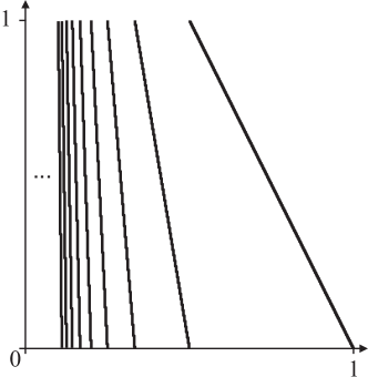
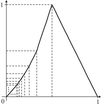
Figure 1.1. The alternating Lüroth and $\alpha_{H}$-Farey map, where $t_{n}=1/n$, $n\in\mathbb{N}$.

The main goal of this paper is to give a thorough analysis of the two maps $F_{\alpha}$ and $L_{\alpha}$. This includes the study of the sequence of $\alpha$-sum-level sets $\left(\mathcal{L}^{(\alpha)}_{n}\right)_{n\in\mathbb{N}}$ arising from the $\alpha$-Lüroth map, for an arbitrary given partition $\alpha$. These sets are defined by

$$\mathcal{L}^{(\alpha)}_{n}:=\left\{x\in C_{\alpha}(\ell_{1},\ell_{2},\ldots,\ell_{k}):\sum_{i=1}^{k}\ell_{i}=n,\hbox{ for some }k\in\mathbb{N}\right\},$$

where $C_{\alpha}(\ell_{1},\ell_{2},\ldots,\ell_{k}):=\{x\in\mathcal{U}:L_{\alpha}^{i-1}(x)\in A_{l_{i}},\text{ for all }i=1,\ldots,k\}$ denotes a cylinder set arising from the map $L_{\alpha}$. The sets $\mathcal{L}^{(\alpha)}_{n}$ can also be written dynamically in terms of $F_{\alpha}$, that is, one immediately verifies that $\mathcal{L}^{(\alpha)}_{n}=F_{\alpha}^{-(n-1)}(A_{1})$, for all $n\in\mathbb{N}$.

Throughout, $\alpha$ is said to be of finite type if for the tails $t_{n}$ of $\alpha$ we have that $\sum_{n=1}^{\infty}t_{n}$ converges, otherwise $\alpha$ is said to be of infinite type. Moreover, a partition $\alpha$ is called expansive of exponent $\theta$ if its tails satisfy the power law $t_{n}=\psi(n)n^{-\theta}$, for all $n\in\mathbb{N}$, for some $\theta\geq 0$ and for some slowly varying function $\psi$. Note that in this situation we have that $\lim_{n\to\infty}t_{n}/t_{n+1}=1$, and hence the right derivative of $F_{\alpha}$ at zero is equal to $1$, which explains why this type of partition is referred to as expansive.

Also, a partition $\alpha$ is said to be expanding if $\lim_{n\to\infty}t_{n}/t_{n+1}=\rho$, for some $\rho>1$. In this situation we have that the right derivative of $F_{\alpha}$ at zero is equal to $\rho$, and that is why we refer to it as expanding (cf. Lemma 4.1 (2)). Clearly, if $\alpha$ is expanding, then $F_{\alpha}$ is of finite type. Furthermore, a partition $\alpha$ is called eventually decreasing if $a_{n+1}\leq a_{n}$, for all $n\in\mathbb{N}$ sufficiently large.

Throughout, we use the notation $a_{n}\sim b_{n}$ to denote $\lim_{n\to\infty}a_{n}/b_{n}=1$.

Theorem 1 (Renewal laws for sum-level sets).

1. For the Lebesgue measure $\lambda(\mathcal{L}^{(\alpha)}_{n})$ of the $\alpha$-sum-level sets of a given partition $\alpha$ of $\mathcal{U}$ we have that $\sum_{n=1}^{\infty}\lambda(\mathcal{L}^{(\alpha)}_{n})$ diverges, and that

   $$\lim_{n\to\infty}\lambda\left(\mathcal{L}^{(\alpha)}_{n}\right)=\left\{\begin{array}[]{ll}0,&\hbox{if $\alpha$ is of infinite type;}\\ \left(\sum_{k=1}^{\infty}t_{k}\right)^{-1},&\hbox{if $\alpha$ is of finite type.}\end{array}\right.$$

2. For a given partition $\alpha$ which is either expansive of exponent $\theta\in[0,1]$ or of finite type, we have the following estimates for the asymptotic behaviour of $\lambda(\mathcal{L}^{(\alpha)}_{n})$.

   1. Weak renewal law. With $K_{\alpha}:=(\Gamma(2-\theta)\Gamma(1+\theta))^{-1}$ for $\alpha$ expansive of exponent $\theta\in[0,1]$, and with $K_{\alpha}:=1$ for $\alpha$ of finite type, we have that

      $$\sum_{k=1}^{n}\lambda\left(\mathcal{L}^{(\alpha)}_{k}\right)\sim K_{\alpha}\,\cdot n\cdot\left(\sum_{k=1}^{n}t_{k}\right)^{-1}.$$

   2. Strong renewal law. With $k_{\alpha}:=(\Gamma(2-\theta)\Gamma(\theta))^{-1}$ for $\alpha$ expansive of exponent $\theta\in(1/2,1]$, and with $k_{\alpha}:=1$ for $\alpha$ of finite type, we have

      $$\lambda\left(\mathcal{L}^{(\alpha)}_{n}\right)\sim k_{\alpha}\cdot\left(\sum_{k=1}^{n}t_{k}\right)^{-1}.$$

Remark 1. Note that, by using a result of Garsia and Lamperti ([10]), we have for an expansive partition $\alpha$ of exponent $\theta\in(0,1)$, that

$$\liminf_{n\to\infty}\left(n\cdot t_{n}\cdot\lambda\left(\mathcal{L}^{(\alpha)}_{n}\right)\right)=\frac{\sin\pi\theta}{\pi}.$$

Moreover, if $\theta\in(0,1/2)$, then the corresponding limit does not exist in general. However, in this situation the existence of the limit is always guaranteed at least on the complement of some set of integers of zero density.

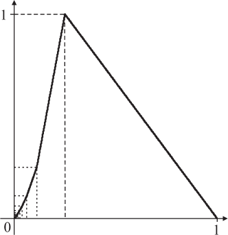
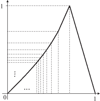
Figure 1.2. The graphs of two $\alpha$-Farey maps with $\alpha$ expansive. The partition on the left is of finite type with $t_{n}=1/n^{2}$, $n\in\mathbb{N}$ and the partition on the right is of infinite type with $t_{n}={1/\sqrt{n}}$, $n\in\mathbb{N}$.

In order to state our remaining main results, recall that the Lyapunov exponent of a differentiable map $S:\mathcal{U}\to\mathcal{U}$ at a point $x\in\mathcal{U}$ is defined, provided the limit exists, by

$$\Lambda(S,x):=\lim_{n\to\infty}\frac{1}{n}\sum_{k=0}^{n-1}\log|S^{\prime}(S^{k}(x))|.$$

Our second main theorem gives a complete fractal-geometric description of the Lyapunov spectra associated with the map $L_{\alpha}$. That is, we consider the spectral sets $\{s\in\mathbb{R}:\{x\in\mathcal{U}:\Lambda(L_{\alpha},x)=s\}\not=\emptyset\}$ associated with the Hausdorff dimension function $\tau_{\alpha}$, which is given by

$$\tau_{\alpha}(s):=\dim_{H}(\{x\in\mathcal{U}:\Lambda(L_{\alpha},x)=s\}).$$

In the following $p:\mathbb{R}\to\mathbb{R}\cup\{\infty\}$ denotes the $\alpha$-Lüroth pressure function, given by $p(u):=\log\sum_{n=1}^{\infty}a_{n}^{u}$. We say that $L_{\alpha}$ exhibits no phase transition if and only if the pressure function $p$ is differentiable everywhere (that is, the right and left derivatives of $p$ coincide everywhere, with the convention that $p^{\prime}(u)=\infty$ if $p(u)=\infty$). We refer to [26] for an interesting further discussion of the phenomenon of phase transition in the context of countable state Markov chains.

Theorem 2 (Lyapunov spectrum for $\alpha$-Lüroth systems).

For a given partition $\alpha$, the Hausdorff dimension function of the Lyapunov spectrum associated with $L_{\alpha}$ is given as follows. For $t_{-}:=\min\{-\log a_{n}:n\in\mathbb{N}\}$ we have that $\tau_{\alpha}$ vanishes on $(-\infty,t_{-})$, and for each $s\in(t_{-},\infty)$ we have

$$\tau_{\alpha}(s)=\inf_{u\in\mathbb{R}}\left(u+s^{-1}p(u)\right).$$

Moreover, $\tau_{\alpha}(s)$ tends to $t_{\infty}:=\inf\{r>0:\sum_{k=1}^{\infty}a_{n}^{r}<\infty\}\leq 1$ for $s$ tending to infinity. Note that $t_{\infty}$ is also equal to the Hausdorff dimension of the Good-type set $G_{\infty}^{(\alpha)}$ associated to $L_{\alpha}$, given by

$$G_{\infty}^{(\alpha)}:=\{[\ell_{1},\ell_{2},\ldots]_{\alpha}:\lim_{n\to\infty}\ell_{n}=\infty\}.$$

Concerning the possibility of phase transitions for $L_{\alpha}$, the following hold:

• If $\alpha$ is expanding, then $L_{\alpha}$ exhibits no phase transition and $t_{\infty}=0$.

• If $\alpha$ is expansive of exponent $\theta>0$ and eventually decreasing, then $L_{\alpha}$ exhibits no phase transition if and only if $\sum_{n=1}^{\infty}\psi(n)^{1/(1+\theta)}(\log n)/n$ diverges. Moreover, in this situation we have that $t_{\infty}=1/(1+\theta)$.

• If $\alpha$ is expansive of exponent $\theta=0$, then $L_{\alpha}$ exhibits no phase transition if and only if $\sum_{n=1}^{\infty}a_{n}\log(a_{n})$ diverges. Moreover, in this situation we have that $t_{\infty}=1$.

Note that the Lyapunov spectra for the Gauss map and the Farey map have been determined in [16]. Also, the sets $G_{\infty}^{(\alpha)}$ are named for I.J. Good [12], for his results concerning similar sets in the continued fraction setting.

In our final main theorem we consider the Lyapunov spectra arising from the maps $F_{\alpha}$. In other words, we consider the spectral sets $\{s\in\mathbb{R}:\{x\in\mathcal{U}:\Lambda(F_{\alpha},x)=s\}\not=\emptyset\}$ associated with the Hausdorff dimension-function $\sigma_{\alpha}(s)$, given by

$$\sigma_{\alpha}(s):=\dim_{H}(\{x\in\mathcal{U}:\Lambda(F_{\alpha},x)=s\}).$$

We define the $\alpha$-Farey free energy function $v:\mathbb{R}\to\mathbb{R}$, to be given by

$$v(u):=\inf\left\{r\in\mathbb{R}:\sum_{n=1}^{\infty}a_{n}^{u}\exp\left(-rn\right)\leq 1\right\}.$$

Note that we will say that $F_{\alpha}$ exhibits no phase transition if and only if the $\alpha$-Farey free energy function $v$ is differentiable everywhere, that is, the right and left derivatives of $v$ coincide everywhere.

Theorem 3 (Lyapunov spectrum for $\alpha$-Farey systems).

Let $\alpha$ be a partition that is either expanding, or expansive and eventually decreasing. The Hausdorff dimension function of the Lyapunov spectrum associated with $F_{\alpha}$ is then given as follows. For $s_{-}:=\inf\{-(\log a_{n})/n:n\in\mathbb{N}\}$ and $s_{+}:=\sup\{-(\log a_{n})/n:n\in\mathbb{N}\}$, we have that $\sigma_{\alpha}\left(s\right)$ vanishes outside the interval $[s_{-},s_{+}]$ and for each $s\in(s_{-},s_{+})$, we have

$$\sigma_{\alpha}\left(s\right)=\inf_{u\in\mathbb{R}}\left(u+s^{-1}v\left(u\right)\right).$$

Concerning the possibility of phase transitions for $F_{\alpha}$, the following hold:

• If $\alpha$ is expanding, then $F_{\alpha}$ exhibits no phase transition. In particular, $v$ is strictly decreasing and bijective.

• If $\alpha$ is expansive of exponent $\theta$ and eventually decreasing, then $F_{\alpha}$ exhibits no phase transition if and only if $\alpha$ is of infinite type. In particular, $v$ is non-negative and vanishes on $[1,\infty)$.

The structure of the paper is as follows. In Section 2, we will collect various basic properties of the $\alpha$-Farey map and the $\alpha$-Lüroth map. In particular, this will include a discussion of the topological dynamics of these two maps and the way in which they give rise to a family of distribution functions which are all in the spirit of the Minkowski question mark function (see [23],[25] and [17]). Then, we will locate the invariant densities associated with the $\alpha$-Farey system and the $\alpha$-Lüroth system and also establish exactness for both of these maps.

In Section 3, we study the sequence of Lebesgue measures of the $\alpha$-sum-level sets, defined above. We first show that this sequence satisfies a renewal-type equation. We then employ the discrete Renewal Theorem by Erdős, Pollard and Feller ([8]), as well some renewal results by Garsia, Lamperti ([10]) and Erickson ([9]), and show how these give rise to the proof of Theorem 1.

In Section 4, we will give a complete description of the multifractal spectra arising from the $\alpha$-Farey map and the $\alpha$-Lüroth map. For this we use a general method obtained in [14]. Furthermore, we give a detailed discussion of the phenomenon of phase transition. These are the main steps in the proofs of Theorem 2 and Theorem 3.

In the Appendix, we will first consider the map $F_{\alpha_{H}}$, arising from the harmonic partition $\alpha_{H}$. As already mentioned above, the associated map $L_{\alpha_{H}}$ coincides with the alternating Lüroth map. We end the paper by giving various further examples which demonstrate the diversity of different behaviours of the spectra given by Theorems 2 and 3 in dependence on the chosen partition $\alpha$.

Remark. Let us briefly comment also on the behaviour of the Lyapunov spectra at their boundary points. Note that in all the examples given at the end of the paper (see Figures 5.1, 5.2, 5.3, 5.4, 5.5 and 5.6) we have that $\sigma_{\alpha}(s_{+})=\tau_{\alpha}(t_{-})=0$. However, in general this is not necessarily true. For instance, one immediately verifies that for a partition $\alpha$ for which $a_{1}=a_{2}$, one has that $\tau_{\alpha}(t_{-})\geq(\log 2)/(-\log a_{1})>0$. Likewise, if $\alpha$ is given such that $a_{1}=\sqrt{a_{2}}$, then $\sigma_{\alpha}(s_{+})\geq(\log((1+\sqrt{5})/2))/(-\log a_{1})>0$. Also note that, if $\alpha$ is a partition which is expanding and eventually decreasing, then we always have that $s_{-}>0$, whereas $\sigma_{\alpha}(s_{-})$ can be either equal to zero or strictly positive. Furthermore, for an expansive partition $\alpha$ we always have that $s_{-}=0$ and $\sigma_{\alpha}(0)=1$. In order to see that $\sigma_{\alpha}(0)=1$ is in fact true for any partition $\alpha$, one argues as follows. On the one hand, if $\alpha$ is of infinite type, then this follows from the fact that $\Lambda(F_{\alpha},x)=0$, for $\lambda$-almost all $x\in\mathcal{U}$. On the other hand, if $\alpha$ is of finite type, then the proof follows along the lines of the proof of [11, Proposition 10].

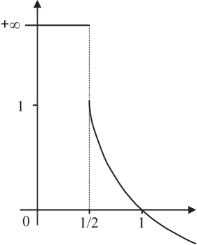
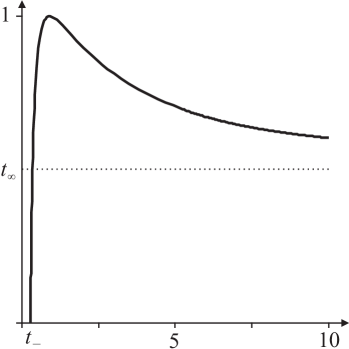
Figure 5.4. Finite critical value ${p(t_{\infty})<\infty}$ and no phase transition for the $\alpha$-Lüroth pressure function and $\alpha$ expansive. The $\alpha$-Lüroth pressure function $p$, and the associated dimension graphs for the $\alpha$-Lüroth system with $a_{n}:=n^{-2}\cdot(\log(n+5))^{-4}/C$, where $C:=\sum_{n\geq 1}n^{-2}\cdot(\log(n+5))^{-4}$. In this case $t_{\infty}=1/2$ and $p(1/2)<\infty$, but $L_{\alpha}$ exhibits no phase transition.

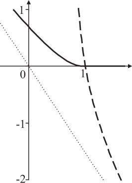
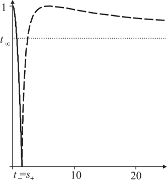
Figure 5.5. The Farey spectrum and the Lüroth spectrum intersect in a single point, for $\alpha$ expansive. The $\alpha$-Farey free energy $v$ (solid line), the $\alpha$-Lüroth pressure function $p$ (dashed line), and the associated dimension graphs for $a_{n}:=\zeta\left(5/4\right)^{-1}n^{-5/4}$. Here, $F_{\alpha}$ exhibits no phase transition.

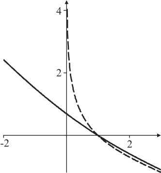
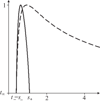
Figure 5.6. The Farey spectrum is completely contained in the Lüroth spectrum, for $\alpha$ expanding. The $\alpha$-Farey free energy $v$ (solid line), the $\alpha$-Lüroth pressure function $p$ (dashed line), and the associated dimension graphs for the $\alpha$-Farey and $\alpha$-Lüroth systems with $a_{n}:=2\cdot 3^{-n}$, $n\in\mathbb{N}$. The $\alpha$-Farey system is given in this situation by the tent map with slopes $3$ and $-3/2$.

Remark 2. Note that for the Farey map and its jump transformation, the Gauss map, the analogue of Theorem 1 has been obtained by the first and the third author in [18]. There the results were derived by using advanced infinite ergodic theory, rather than the strong renewal theorems employed in this paper. This underlines the fact that one of the main ingredients of infinite ergodic theory is provided by some delicate estimates in renewal theory. Likewise, as already mentioned above, the Lyapunov spectra for the Farey map and the Gauss map have been investigated in detail in [16]. The results there are parallel to the outcomes of Theorem 2 and 3. Clearly, the Farey map and the Gauss map are non-linear, whereas the systems in this paper are always piecewise linear. However, since our analysis is based on a large family of different partitions of $\mathcal{U}$, the class of maps which we consider in this paper allows to detect a variety of interesting new phenomena. For instance, as shown in [16], the spectral sets of the Farey map and the Gauss map intersect at the single point $2\log((\sqrt{5}+1)/2)$. The same type of behaviour can also be found in our piecewise linear setting, as shown in Fig. 5.5 for $a_{n}:=\zeta\left(5/4\right)^{-1}n^{-5/4}$, where $\zeta$ denotes the Riemann zeta-function. However, this situation is by no means canonical, as the harmonic partition $\alpha_{H}$ already shows, where the intersection of the two spectral sets is equal to the interval $[\log 2,(\log 6)/2]$ (cf. Fig. 5.1). The situation can be even more dramatic, as shown in Fig. 5.6 for the partition $\alpha$ determined by $a_{n}:=2\cdot 3^{-n}$. For this partition, the spectral set associated with the $\alpha$-Farey map is fully contained in the spectral set of the $\alpha$-Lüroth map. A similar picture arises when one considers the possibility of the existence of phase transitions. The results of [16] clearly show that neither the Gauss map nor the Farey map exhibit the type of phase transition established in this paper. In contrast to this, Theorem 2 and 3 show that in the piecewise linear scenario the situation is much more interesting, as the examples in Fig. 5.2, 5.3 and 5.4 clearly demonstrate. More specifically, if $\lim_{r\searrow t_{\infty}}\sum_{n=1}^{\infty}a_{n}^{r}\log a_{n}/\sum_{n=1}^{\infty}a_{n}^{r}=\infty$ then the dimension function $\tau_{\alpha}$ is real-analytic on $\left(t_{-},\infty\right)$. An example for this is provided by the alternating Lüroth system, where $a_{n}=\left(n\left(n+1\right)\right)^{-1}$, and hence, $t_{\infty}=1/2$ and $\sum_{n=1}^{\infty}a_{n}^{t_{\infty}}=\infty$ (cf. Fig. 5.1, see also Fig. 5.2, 5.5, and 5.6 for further examples). Note that the example considered in Fig. 5.4 is particularly interesting, since it shows that it is possible that there is no phase transition, although $p(t_{\infty})$ is finite. That is, for $a_{n}:=(n\left(\log n\right)^{2})^{-2}/\sum_{k=1}^{\infty}(k\left(\log k\right)^{2})^{-2}$, we have on the one hand $\sum_{n=1}^{\infty}a_{n}^{t_{\infty}}<\infty$ with $t_{\infty}=1/2$, but on the other hand we have $\lim_{t\searrow t_{\infty}}\sum_{n=1}^{\infty}a_{n}^{t}\log a_{n}/\sum_{n=1}^{\infty}a_{n}^{t}=\infty$. However, for a partition $\alpha$ for which $t_{0}:=\lim_{t\searrow t_{\infty}}\sum_{n=1}^{\infty}a_{n}^{t}\log a_{n}/\sum_{n=1}^{\infty}a_{n}^{t}<\infty$, the $\alpha$-Lüroth map $L_{\alpha}$ exhibits a phase transition of the first kind at $t_{\infty}$. In this case the Hausdorff dimension function $\tau_{\alpha}$ is real-analytic on $\left(t_{-},t_{0}\right)$, whereas for $t\in[t_{0},+\infty)$ it is explicitly given by

$$\tau_{\alpha}(t)=\frac{\sum_{n=1}^{\infty}a_{n}^{t_{\infty}}}{t}+t_{\infty}.$$

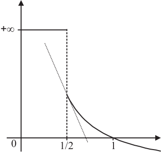
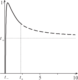
Figure 5.3. Finite critical value ${p(t_{\infty})<\infty}$ with phase transition for the $\alpha$-Lüroth pressure function and $\alpha$ expansive. The $\alpha$-Lüroth pressure function $p$, and the associated dimension graphs for the $\alpha$-Lüroth system with $a_{n}:=n^{-2}\cdot(\log(n+5))^{-12}/C$, where $C:=\sum_{n\geq 1}n^{-2}\cdot(\log(n+5))^{-12}$. In this case $t_{\infty}=1/2$ and $p(1/2)<\infty$ and $L_{\alpha}$ has a phase transition, namely, $v$ is not differentiable at $1/2$.

An example demonstrating the latter situation is given in Fig. 5.3.

2. Preliminary discussion of $F_{\alpha}$ and $L_{\alpha}$

Throughout this section we let $\alpha$ denote some arbitrary partition of $\mathcal{U}$ of the type specified at the beginning of the introduction.

2.1. Topological properties of $F_{\alpha}$ and $L_{\alpha}$

Recall from the introduction that the $\alpha$-Lüroth map $L_{\alpha}$ is given by

$$L_{\alpha}(x):=\left\{\begin{array}[]{ll}({t_{n}-x})/a_{n},&\text{ if }x\in A_{n},\ n\in\mathbb{N},\\ 0,&\hbox{ if }x=0.\end{array}\right.$$

In the same way as the Gauss map gives rise to the continued fraction expansion, the map $L_{\alpha}$ gives rise to a series expansion of numbers in the unit interval, which we refer to as the $\alpha$-Lüroth expansion. More precisely, let $x\in\mathcal{U}\setminus\{0\}$ be given and let the finite or infinite sequence $(\ell_{k})_{k\geq 1}$ of positive integers be determined by $L_{\alpha}^{k-1}(x)\in A_{\ell_{k}}$, where the sequence terminates in $k$ if and only if $L_{\alpha}^{k-1}(x)=t_{n}$, for some $n\geq 2$. Then the $\alpha$-Lüroth expansion of $x$ is given as follows, where the sum is supposed to be finite if the sequence is finite.

$$x=\sum_{n=1}^{\infty}(-1)^{n-1}\left(\textstyle\prod\limits_{i<n}a_{\ell_{i}}\right)t_{\ell_{n}}=t_{\ell_{1}}-a_{\ell_{1}}t_{\ell_{2}}+a_{\ell_{1}}a_{\ell_{2}}t_{\ell_{3}}+\cdots$$

In this situation we then write $x=:[\ell_{1},\ell_{2},\ell_{3},\ldots]_{\alpha}$. It is easy to see that every infinite expansion is unique, whereas each $x\in(0,1)$ with a finite $\alpha$-Lüroth expansion can be expanded in exactly two ways. Namely, one immediately verifies that $x=[\ell_{1},\ldots,\ell_{k},1]_{\alpha}=[\ell_{1},\ldots,\ell_{k-1},(\ell_{k}+1)]_{\alpha}$. Note that the map $L_{\alpha}$ only provides the latter expression. By analogy with continued fractions, for which a number is rational if and only if it has a finite continued fraction expansion, we say that $x\in\mathcal{U}$ is an $\alpha$-rational number when $x$ has a finite $\alpha$-Lüroth expansion and say that $x$ is an $\alpha$-irrational number otherwise. Of course, the set of $\alpha$-rationals is a countable set.

If we truncate the $\alpha$-Lüroth expansion of $x$ after $k$ entries we obtain the $k$-th convergent of $x$, denoted $r_{k}^{(\alpha)}(x)$, which is given by

$$r_{k}^{(\alpha)}(x):=[\ell_{1},\ldots,\ell_{k}]_{\alpha}=t_{\ell_{1}}-a_{\ell_{1}}t_{\ell_{2}}+\cdots+(-1)^{k-1}\left(\prod_{i=1}^{k-1}a_{\ell_{i}}\right)t_{\ell_{k}}.$$

Note that if $x=[\ell_{1},\ell_{2},\ell_{3},\ldots]_{\alpha}$, then $L_{\alpha}(x)=[\ell_{2},\ell_{3},\ell_{4},\ldots]_{\alpha}$. This shows that, topologically, $L_{\alpha}$ corresponds to the shift map on the space $\mathbb{N}^{\mathbb{N}}$, at least for those points with an infinite $\alpha$-Lüroth expansion. The cylinder sets associated with the $\alpha$-Lüroth expansion are denoted by

$$C_{\alpha}(\ell_{1},\ldots,\ell_{k}):=\{[x_{1},x_{2},\ldots]_{\alpha}:x_{i}=\ell_{i}\text{ for }i=1,\ldots,k\}.$$

We remark here that these cylinder sets are closed intervals with endpoints given by $[\ell_{1},\ldots,\ell_{k}]_{\alpha}$ and $[\ell_{1},\ldots,\ell_{k-1},(\ell_{k}+1)]_{\alpha}$. Consequently, we have for the Lebesgue measure of $C_{\alpha}(\ell_{1},\ldots,\ell_{k})$ that

$$\lambda(C_{\alpha}(\ell_{1},\ldots,\ell_{k}))=\prod_{i=1}^{k}a_{\ell_{i}}.$$

For the first lemma of this section, recall that the jump transformation $F_{\alpha}^{*}:\mathcal{U}\to\mathcal{U}$ of $F_{\alpha}$ is given by $F_{\alpha}^{*}(x)=F_{\alpha}^{\rho_{\alpha}(x)}(x)$, where $\rho_{\alpha}:\mathcal{U}\to\mathbb{N}$ is given by $\rho_{\alpha}(x):=\inf\{n\geq 0:F_{\alpha}^{n}(x)\in A_{1}\}+1$. Note that one can immediately verify that $\rho_{\alpha}(x)$ is finite for all $x\in\mathcal{U}\setminus\{0\}$.

Lemma 2.1.

The jump transformation $F_{\alpha}^{*}$ of the $\alpha$-Farey map $F_{\alpha}$ coincides with the $\alpha$-Lüroth map $L_{\alpha}$.

Proof.

First note that if $x=[1,\ell_{2},\ell_{3},\ldots]_{\alpha}\in A_{1}$, for some $\ell_{2},\ell_{3},\ldots\in\mathbb{N}$, then $\rho_{\alpha}(x)$ is clearly equal to $1$. Thus, $F_{\alpha}^{*}(x)=F_{\alpha}(x)$, which is equal to $L_{\alpha}(x)$, since $L_{\alpha}|_{A_{1}}=F_{\alpha}|_{A_{1}}$.

Secondly, for $n\geq 2$ we have that $x\in A_{n}$ if and only if $x=[n,\ell_{2},\ell_{3},\ldots]_{\alpha}$, for some $\ell_{2},\ell_{3},\ldots\in\mathbb{N}$. We then have that

$$F_{\alpha}^{*}(x)=F_{\alpha}^{n}([n,\ell_{2},\ell_{3},\ldots]_{\alpha})=F_{\alpha}^{n-1}([n-1,\ell_{2},\ell_{3},\ldots]_{\alpha})=\cdots=[\ell_{2},\ell_{3},\ldots]_{\alpha}=L_{\alpha}(x).$$

∎

Let us now describe a Markov partition $\alpha^{*}$ and its associated coding for the map $F_{\alpha}$. The partition $\alpha^{*}$ is equal to $\{A,B\}$, where $A:=A_{1}$ and $B:=\mathcal{U}\setminus A_{1}$. Each $x\in\mathcal{U}$ has an infinite Markov coding $x=\langle x_{1},x_{2},\ldots\rangle_{\alpha}\in\{0,1\}^{\mathbb{N}}$, which, for each positive integer $k$, is given by $x_{k}=1$ if and only if $F_{\alpha}^{k-1}(x)\in A$. This coding will be referred to as the $\alpha$-Farey coding. The associated cylinder sets are denoted by

$$\widehat{C}_{\alpha}(x_{1},\ldots,x_{n}):=\{\langle y_{1},y_{2},\ldots\rangle_{\alpha}:y_{k}=x_{k},\text{ for }k=1,\ldots,n\}.$$

Notice that all of the $\alpha$-Lüroth cylinder sets are also $\alpha$-Farey cylinder sets, whereas the converse of this is not true. More precisely, a given $\alpha$-Farey cylinder set $\widehat{C}_{\alpha}(0^{\ell_{1}-1}10^{\ell_{2}-1}10^{\ell_{3}-1}\cdots 0^{\ell_{k}-1}1)$ coincides with the $\alpha$-Lüroth cylinder set $C_{\alpha}(\ell_{1},\ldots,\ell_{k})$. Moreover, if the coding of an $\alpha$-Farey cylinder set ends in a $0$, then it cannot be represented by a single $\alpha$-Lüroth cylinder set.

In the sequel, we require the inverse branches $F_{\alpha,0}$ and $F_{\alpha,1}$ of the map $F_{\alpha}$. With the convention that $F_{\alpha,0}(0)=0$, it is straightforward to calculate that these are given by $F_{\alpha,1}(x):=1-{a_{1}}x$ for $x\in{\mathcal{U}}$ and

$$F_{\alpha,0}(x):=\frac{a_{n+1}}{a_{n}}(x-t_{n+1})+t_{n+2}\;\text{ for }\;x\in A_{n},n\in\mathbb{N}.$$

In preparation for the next lemma, we now describe the $\alpha$-Farey decomposition of the interval $\mathcal{U}$, which is obtained by iterating the maps $F_{\alpha,0}$ and $F_{\alpha,1}$ on $\mathcal{U}$. The first iteration gives rise to the partition $\{\widehat{C}_{\alpha}(0),\widehat{C}_{\alpha}(1)\}$. Iterating a second time yields the refined partition $\{\widehat{C}_{\alpha}(00),\widehat{C}_{\alpha}(01),\widehat{C}_{\alpha}(11),\widehat{C}_{\alpha}(10)\}$. Continuing the iteration further, we obtain successively refined partitions of $\mathcal{U}$ consisting of $2^{k}$ $\alpha$-Farey cylinder sets of the form $\widehat{C}_{\alpha}(x_{1},\ldots,x_{k})$, for every $k\in\mathbb{N}$. It is clear that exactly half of these are also $\alpha$-Lüroth cylinder sets. The endpoints of each of these so-obtained intervals are $\alpha$-rational numbers, and every $\alpha$-rational number is obtained in this way. Finally, note that if $x=[\ell_{1},\ell_{2},\ldots]_{\alpha}$, then

$$F_{\alpha}(x):=\left\{\begin{array}[]{ll}[\ell_{1}-1,\ell_{2},\ell_{3},\ldots]_{\alpha},&\hbox{for $\ell_{1}\geq 2$;}\\ [\ell_{2},\ell_{3},\ldots]_{\alpha},&\hbox{for $\ell_{1}=1$.}\end{array}\right.$$

Also observe that if we consider the dyadic partition $\alpha_{D}$ given by $a_{n}:=2^{-n}$, then the map $F_{\alpha_{D}}$ arising from this particular partition turns out to coincide with the tent map, given by

$$F_{\alpha_{D}}(x):=\left\{\begin{array}[]{ll}2x&\hbox{for $x\in[0,1/2)$;}\\ 2-2x&\hbox{for $x\in[1/2,1]$.}\end{array}\right.$$

Before stating the lemma, we remind the reader that the measure of maximal entropy $\mu_{\alpha}$ for the system $F_{\alpha}$ is the measure that assigns mass $2^{-n}$ to each $n$-th level $\alpha$-Farey cylinder set.

Lemma 2.2.

The dynamical systems $(\mathcal{U},{F}_{\alpha})$ and $(\mathcal{U},F_{\alpha_{D}})$ are topologically conjugate and the conjugating homeomorphism is given, for each $x=[\ell_{1},\ell_{2},\ldots]_{\alpha}$, by

$${\theta_{\alpha}}(x):=-2\sum_{k=1}^{\infty}(-1)^{k}2^{-\sum_{i=1}^{k}\ell_{i}}.$$

Moreover, the map $\theta_{\alpha}$ is equal to the distribution function of the measure of maximal entropy $\mu_{\alpha}$ for the $\alpha$-Farey map.

Proof.

We will first show by induction that the map $\theta_{\alpha}$ is indeed equal to the distribution function $\Delta_{\mu_{\alpha}}$ of the measure $\mu_{\alpha}$. To start, observe that $\Delta_{\mu_{\alpha}}([1]_{\alpha})=1=\theta_{\alpha}([1]_{\alpha})$ and notice that for each $k\geq 2$ the $\alpha$-rational number $[k]_{\alpha}$ appears for the first time in the $(k-1)$-th level of the $\alpha$-Farey decomposition, as the right endpoint of the cylinder set $\widehat{C}_{\alpha}(0,\ldots,0)$, with code consisting of $k-1$ zeros. By the definition of the measure of maximal entropy, we have that $\Delta_{\mu_{\alpha}}([k]_{\alpha})=2^{-(k-1)}={\theta_{\alpha}}([k]_{\alpha})$.

Now, suppose that $\Delta_{\mu_{\alpha}}([\ell_{1},\ell_{2},\ldots,\ell_{k}]_{\alpha})=\theta_{\alpha}([\ell_{1},\ell_{2},\ldots,\ell_{k}]_{\alpha})$ for every $k$-tuple of positive integers $\ell_{1},\ldots,\ell_{k}$ and each $1\leq k\leq n$, for some $n\in\mathbb{N}$. Further suppose that $n$ is even. (The case where $n$ is odd proceeds similarly.) We then have that the points $[\ell_{1},\ell_{2},\ldots,\ell_{n}]_{\alpha}$ and $[\ell_{1},\ell_{2},\ldots,\ell_{n},1]_{\alpha}$ are, respectively, the left and the right endpoints of the $\left(\sum_{i=1}^{n}\ell_{i}\right)$-th level $\alpha$-Farey cylinder set $\widehat{C}_{\alpha}(0^{\ell_{1}-1}10^{\ell_{2}-1}1\cdots 0^{\ell_{n}-1}1)$. Clearly, this cylinder set has $\mu_{\alpha}$-measure equal to $2^{-\sum_{i=1}^{n}\ell_{i}}$. Similarly, we have that the interval bounded by $[\ell_{1},\ell_{2},\ldots,\ell_{n}]_{\alpha}$ and $[\ell_{1},\ell_{2},\ldots,\ell_{n},2]_{\alpha}$ is a $\alpha$-Farey cylinder set of level $\left(\sum_{i=1}^{n}\ell_{i}\right)+1$ and as such, has $\mu_{\alpha}$-measure equal to $2^{-\sum_{i=1}^{n}\ell_{i}-1}$. Continuing in this way, we reach the interval bounded by the points $[\ell_{1},\ell_{2},\ldots,\ell_{n}]_{\alpha}$ and $[\ell_{1},\ell_{2},\ldots,\ell_{n},\ell_{n+1}]_{\alpha}$, which has $\mu_{\alpha}$-measure equal to $2^{-\sum_{i=1}^{n+1}\ell_{i}+1}$.

Using this, we are now in a position to finish the proof by induction, as follows.

$$\Delta_{\mu_{\alpha}}([\ell_{1},\ldots,\ell_{n},\ell_{n+1}]_{\alpha})$$

$$= \Delta_{\mu_{\alpha}}([\ell_{1},\ldots,\ell_{n}]_{\alpha})+\mu_{\alpha}(([\ell_{1}\ldots,\ell_{n}]_{\alpha},[\ell_{1},\ldots,\ell_{n},\ell_{n+1}]_{\alpha}))$$

$$= \theta_{\alpha}([\ell_{1},\ldots,\ell_{n}]_{\alpha})+2^{-\sum_{i=1}^{n+1}\ell_{i}+1}=\theta_{\alpha}([\ell_{1},\ldots,\ell_{n},\ell_{n+1}]_{\alpha}).$$

It remains to show that the map $\theta_{\alpha}$ is the conjugating homeomorphism from $F_{\alpha}$ to the tent system. For this, suppose first that $x=[\ell_{1},\ell_{2},\ldots]_{\alpha}\in\mathcal{U}\setminus A_{1}$. Then, $\theta_{\alpha}(x)$ is an element of $[0,1/2]$ and we have that

$$F_{\alpha_{D}}\left(\theta_{\alpha}(x)\right) = 2\left(-2\sum_{k=1}^{\infty}(-1)^{k}2^{-\sum_{i=1}^{k}\ell_{i}}\right)=-2\left(\sum_{k=1}^{\infty}(-1)^{k}2^{-(\ell_{1}-1)-\sum_{i=2}^{k}\ell_{i}}\right)$$

$$= \theta_{\alpha}\left([\ell_{1}-1,\ell_{2},\ell_{3},\ldots]_{\alpha}\right)=\theta_{\alpha}(F_{\alpha}(x)).$$

Now, suppose that $x\in A_{1}$, that is, $x=[1,\ell_{2},\ell_{3},\ldots]_{\alpha}$. Then, it follows that $\theta_{\alpha}(x)\in[1/2,1]$ and we have that

$$F_{\alpha_{D}}(\theta_{\alpha}(x)) = 2-2\left(2\cdot 2^{-1}-2\sum_{k=2}^{\infty}(-1)^{k}2^{-1-\sum_{i=2}^{k}\ell_{i}}\right)$$

$$= -2\left(\sum_{k=2}^{\infty}(-1)^{k}2^{\sum_{i=2}^{k}\ell_{i}}\right)=\theta_{\alpha}\left([\ell_{2},\ell_{3},\ldots]_{\alpha}\right)=\theta_{\alpha}(F_{\alpha}(x)).$$

∎

Our next aim is to determine the Hölder exponent and the sub-Hölder exponent of the map $\theta_{\alpha}$, for an arbitrary partition $\alpha$. For this, we define $\kappa(n):=-n\log 2/(\log a_{n})$ and set

$$\kappa_{+}:=\inf\left\{\kappa(n):n\in\mathbb{N}\right\}\hbox{ and }\kappa_{-}:=\sup\left\{\kappa(n):n\in\mathbb{N}\right\}.$$

Note that for $\kappa\in(0,\infty)$ a map $S:\mathcal{U}\to\mathcal{U}$ is called $\kappa$-sub-Hölder continuous if there exists a constant $c>0$ such that $|S(x)-S(y)|\geq c|x-y|^{\kappa}$, for all $x,y\in\mathcal{U}$.

Lemma 2.3.

We have that the map $\theta_{\alpha}$ is $\kappa_{+}$-Hölder continuous and $\kappa_{-}$-sub-Hölder continuous.

Proof.

In order to calculate the Hölder exponent of $\theta_{\alpha}$, first note that

$$|\theta_{\alpha}(C_{\alpha}(\ell_{1},\ell_{2},\ldots,\ell_{k}))|=2^{-\sum_{j=1}^{k}\ell_{j}}.$$

This can be seen by simply calculating the image of the endpoints of this cylinder, or by noting that every $\alpha$-Lüroth cylinder $C_{\alpha}(\ell_{1},\ell_{2},\ldots,\ell_{k})$ is an $n$-th level $\alpha$-Farey cylinder, where $\sum_{j=1}^{k}\ell_{j}=n$. For the same reason, we have that $\mu_{\alpha}(C_{\alpha}(\ell_{1},\ell_{2},\ldots,\ell_{k}))=|\theta_{\alpha}(C_{\alpha}(\ell_{1},\ell_{2},\ldots,\ell_{k}))|$, where $\mu_{\alpha}$ again denotes the measure of maximal entropy associated to the map $F_{\alpha}$. Suppose first that $\kappa_{+}$ is non-zero. In that case, we have,

$$\lambda(C_{\alpha}(\ell_{1},\ell_{2},\ldots,\ell_{k})) = \prod_{i=1}^{k}a_{\ell_{i}}=\prod_{i=1}^{k}2^{-\ell_{i}/\kappa(\ell_{i})}\geq\left(\prod_{i=1}^{k}2^{-\ell_{i}}\right)^{1/\kappa_{+}}$$

$$= \left(2^{-\sum_{i=1}^{k}\ell_{i}}\right)^{1/\kappa_{+}}=|\theta_{\alpha}(C_{\alpha}(\ell_{1},\ell_{2},\ldots,\ell_{k}))|^{1/\kappa_{+}}.$$

Or, in other words,

$$|\theta_{\alpha}(C_{\alpha}(\ell_{1},\ell_{2},\ldots,\ell_{k}))|\leq\lambda(C_{\alpha}(\ell_{1},\ell_{2},\ldots,\ell_{k}))^{\kappa_{+}}.$$

Now, let $x$ and $y$ be some arbitrary $\alpha$-irrational numbers in $\mathcal{U}$. There must be a first time during the backwards iteration of $\mathcal{U}$ under the inverse branches of $F_{\alpha}$ in which an $\alpha$-Farey cylinder set appears between the numbers $x$ and $y$. Say that this cylinder set appears in the $p$-th stage of the $\alpha$-Farey decomposition. If we go on iterating one more time, it is clear that there are two $(p+1)$-th level $\alpha$-Farey intervals fully contained in the interval $(x,y)$; moreover, one of these also has to be an $\alpha$-Lüroth cylinder set. Let this $\alpha$-Lüroth cylinder set be denoted by $C_{\alpha}(\ell_{1},\ell_{2},\ldots,\ell_{k})$, where $\sum_{j=1}^{k}\ell_{j}=p+1$. This leads to the observation that, as $C_{\alpha}(\ell_{1},\ell_{2},\ldots,\ell_{k})$ is contained in $(x,y)$,

$$|x-y|^{\kappa_{+}}>\lambda(C_{\alpha}(\ell_{1},\ell_{2},\ldots,\ell_{k}))^{\kappa_{+}}\geq|\theta_{\alpha}(C_{\alpha}(\ell_{1},\ell_{2},\ldots,\ell_{k}))|=2^{-\sum_{j=1}^{k}\ell_{j}}.$$

Consider the interval $(x,y)$ again. It is contained inside two neighbouring $(p-1)$-th level $\alpha$-Farey intervals, and so

$$|\theta_{\alpha}(x)-\theta_{\alpha}(y)|<2^{-(p-1)}+2^{-(p-1)}=2^{-(p-2)}=8\cdot 2^{-(p+1)}.$$

Combining these observations, we obtain that

$$|\theta_{\alpha}(x)-\theta_{\alpha}(y)|\leq 8|x-y|^{\kappa_{+}}.$$

In case $\kappa_{+}$ is equal to zero, we have that there exists $m\in\mathbb{N}$ with the property that

$$\kappa(m)=\frac{m\log 2}{-\log a_{m}}<\frac{1}{q},$$

that is,

$$a_{m}<\mathrm{e}^{-mq\log 2}.$$

So we have that the sequence of partition elements are eventually exponentially decaying, and hence, the Hölder exponent of the map $\theta_{\alpha}$ is necessarily equal to zero.

The proof of the $\kappa_{-}$-sub-Hölder continuity of $\theta_{\alpha}$ follows by similar means and is therefore left to the reader. ∎

Remark. Note that the thermodynamical significance of the Hölder and sub-Hölder exponents of $\theta_{\alpha}$ is that they provide the extreme points of the region $(s_{-},s_{+})$ on which the Hausdorff dimension function $\sigma_{\alpha}$ of $F_{\alpha}$ is non-zero (see Theorem 3). More precisely, we have that

$$\kappa_{-}=\frac{\log 2}{s_{-}}\hbox{ and }\kappa_{+}=\frac{\log 2}{s_{+}},$$

where $\kappa_{-}=\infty$ if and only if $s_{-}=0$.

2.2. Ergodic theoretic properties of $F_{\alpha}$ and $L_{\alpha}$

Let us begin this subsection by showing that $L_{\alpha}$ is an exact transformation and specifying its invariant measure. For this the reader might like to recall that a non-singular transformation $T$ of a $\sigma$–finite measure space $\left(\mathcal{U},\mathcal{B},\mu\right)$ is said to be exact if for each $B\in\bigcap_{n\in\mathbb{N}}T^{-n}\left(\mathcal{B}\right)$ we have that either $\mu(B)$ or $\mu(\mathcal{U}\setminus B)$ vanishes.

Lemma 2.4.

The $\alpha$-Lüroth map $L_{\alpha}$ is measure preserving and exact with respect to $\lambda$.

Proof.

For the proof of $L_{\alpha}$-invariance, let $L_{\alpha,n}$ denote the inverse branch of $L_{\alpha}$ associated with the $n$-th atom $A_{n}$ of $\alpha$. These branches are given by $L_{\alpha,n}(x):=-a_{n}x+t_{n}$, for all $n\in\mathbb{N}$ and $x\in[0,1)$. Then, a straightforward calculation shows that for each element $B$ of the Borel $\sigma$-algebra ${\mathcal{B}}$ on $\mathcal{U}$,

$$\lambda(L_{\alpha}^{-1}(B))=\sum_{n\in\mathbb{N}}\lambda(L_{\alpha,n}(B))=\sum_{n\in\mathbb{N}}a_{n}\lambda(B)=\lambda(B).$$

This gives the $L_{\alpha}$-invariance of $\lambda$.

The proof of exactness is an adaptation of the proof of Kolmogorov’s zero-one law for the one-sided Bernoulli shift (see [19]). To see this, let $B\in\bigcap_{n\in\mathbb{N}}L_{\alpha}^{-n}\left(\mathcal{B}\right)$ be given such that $\lambda(B)>0$. Then, there exists a sequence of Borel sets $(B_{n})_{n\in\mathbb{N}}$ such that $B_{n}\in\mathcal{B}$ and $B=L_{\alpha}^{-n}B_{n}$, for all $n\in\mathbb{N}$. Note that for every finite union $\mathcal{C}$ of $L_{\alpha}$-cylinder sets we have that

$$\lambda(B\cap\mathcal{C})=\lambda(B)\lambda(\mathcal{C}).$$

Indeed, since $\lambda(B)=\lambda(B_{n})$ for all $n\in\mathbb{N}$, if $m$ is the maximal length of the cylinder sets in $\mathcal{C}$, then

$$\lambda(\mathcal{C}\cap B)=\lambda(\mathcal{C}\cap L_{\alpha}^{-m}B_{m})=\lambda(\mathcal{C})\lambda(B_{m})=\lambda(\mathcal{C})\lambda(B).$$

From this we deduce that

$$\lambda(B\cap C)=\lambda(B)\lambda(C),\hbox{ for all }C\in\mathcal{B}.$$

Therefore, by choosing $C=\mathcal{U}\setminus B$, we conclude that

$$0=\lambda(B\cap(\mathcal{U}\setminus B))=\lambda(B)\lambda(\mathcal{U}\setminus B).$$

This shows that $\lambda(B)=1$, and hence finishes the proof. ∎

Since exactness clearly implies ergodicity, the following list of properties of the system $(\mathcal{U},\mathcal{B},L_{\alpha},\lambda)$ is derived from routine ergodic theoretical arguments, and therefore the proofs are left to the reader.

For $\lambda$-almost every $x\in\mathcal{U}$, we have that:

• $\displaystyle{\lim_{n\to\infty}\frac{1}{n}\#\{j\leq n:\ell_{j}(x)=k\}=a_{k}.}$

• $\displaystyle{\lim_{n\to\infty}\frac{1}{n}\log\left(\prod_{j=1}^{n}\ell_{j}(x)\right)=\sum_{k=1}^{\infty}a_{k}\log k.}$

• $\displaystyle{\lim_{n\to\infty}\frac{1}{n}\sum_{j=1}^{n}\ell_{j}(x)=\sum_{k=1}^{\infty}t_{k}.}$

• $\displaystyle{\lim_{n\to\infty}\frac{1}{n}\log\left|x-r_{n}^{(\alpha)}(x)\right|=\sum_{k=1}^{\infty}a_{k}\log a_{k}.}$

We now turn our attention to the ergodic theoretical properties of the $\alpha$-Farey system. The first property to note is that $F_{\alpha}$ is a conservative transformation. This can be seen, for instance, by observing that $\bigcup_{n=0}^{\infty}F_{\alpha}^{-n}(A_{1})=\mathcal{U}\setminus\{0\}$, and hence, Maharam’s Recurrence Theorem ([1, Theorem 1.1.7]) applies, giving that $F_{\alpha}$ is conservative.

Recall that a $\lambda$-absolutely continuous measure $\nu$ on $\mathcal{U}$ is called $F_{\alpha}$-invariant if $\nu\circ F_{\alpha}^{-1}=\nu$, or, equivalently, if $\mathcal{F}_{\alpha}\left(\mathbbm{1}_{\mathcal{U}}\right)=\mathbbm{1}_{\mathcal{U}}$, where $\mathcal{F}_{\alpha}:L^{1}\left(\nu\right)\to L^{1}\left(\nu\right)$ denotes the transfer operator associated with the $\alpha$-Farey system. This is a positive linear operator given by

$$\int_{B}\mathcal{F}_{\alpha}(f)\ d\nu=\int_{F_{\alpha}^{-1}(B)}f\ d\nu,\mbox{ for all }f\in L^{1}\left(\nu\right)\text{ and }B\in\mathcal{B}.$$

Also, note that the Ruelle operator $\mathcal{R}_{\alpha}:L^{1}\left(\nu\right)\to L^{1}\left(\nu\right)$ for the $\alpha$-Farey system is given by

$$\mathcal{R}_{\alpha}\left(f\right)=\left|{F_{\alpha,0}}^{\prime}\right|\cdot\left(f\circ F_{\alpha,0}\right)+\left|{F_{\alpha,1}}^{\prime}\right|\cdot\left(f\circ F_{\alpha,1}\right),\mbox{ for all }f\in L^{1}\left(\nu\right).$$

With $\psi:=d\nu/d\lambda$ denoting the density of $\nu$, one immediately verifies that $\mathcal{F}_{\alpha}$ and $\mathcal{R}_{\alpha}$ are related in the following way:

$$\mathcal{F}_{\alpha}(f)=\frac{1}{\psi}\cdot\mathcal{R}_{\alpha}\left(\psi\cdot f\right),\mbox{ for all }f\in L^{1}\left(\nu\right).$$

So, in order to verify that a particular function $\psi$ is a density which gives rise to an invariant measure for the map $F_{\alpha}$, it is sufficient to show that $\psi$ is an eigenfunction of $\mathcal{R}_{\alpha}$.

Lemma 2.5.

Up to multiplication by a constant, there exists a unique $\lambda$-absolutely continuous invariant measure $\nu_{\alpha}$ for the system $(\mathcal{U},\mathcal{B},F_{\alpha})$. The density $\varphi_{\alpha}$ of $\nu_{\alpha}$ is given, up to multiplication by a constant, by

$$\varphi_{\alpha}:=\frac{d\nu_{\alpha}}{d\lambda}=\sum_{n=1}^{\infty}\frac{t_{n}}{a_{n}}\cdot\mathbbm{1}_{A_{n}}.$$

Moreover, $\nu_{\alpha}$ is a $\sigma$-finite measure, and we have that $\nu_{\alpha}$ is an infinite measure if and only if $\alpha$ is of infinite type.

Proof.

Recall that the inverse branches $F_{\alpha,1}$ and $F_{\alpha,0}$ were defined in Section 2.1 above and note that a straightforward computation shows that for these we have that

$$\varphi_{\alpha}\circ F_{\alpha,1}=t_{1}/a_{1}\cdot\mathbbm{1}_{\mathcal{U}}\hbox{ and }\varphi_{\alpha}\circ F_{\alpha,0}=\sum_{n=1}^{\infty}t_{n+1}/a_{n+1}\cdot\mathbbm{1}_{A_{n}}.$$

Moreover, one immediately verifies that

$$|F_{\alpha,1}^{\prime}|=a_{1}\cdot\mathbbm{1}_{\mathcal{U}}\hbox{ and }|F_{\alpha,0}^{\prime}|=\sum_{n=1}^{\infty}a_{n+1}/a_{n}\cdot\mathbbm{1}_{A_{n}}.$$

Using these two observations, it follows that

$$\mathcal{R}_{\alpha}(\varphi_{\alpha}) = |{F_{\alpha,0}}^{\prime}|\cdot(\varphi_{\alpha}\circ F_{\alpha,0})+|{F_{\alpha,1}}^{\prime}|\cdot(\varphi_{\alpha}\circ F_{\alpha,1})$$

$$= t_{1}\cdot\mathbbm{1}_{\mathcal{U}}+\sum_{n=1}^{\infty}\left(\frac{a_{n+1}}{a_{n}}\frac{t_{n+1}}{a_{n+1}}\right)\cdot\mathbbm{1}_{A_{n}}$$

$$= \sum_{n=1}^{\infty}\left(\frac{t_{n+1}}{a_{n}}+1\right)\cdot\mathbbm{1}_{A_{n}}=\sum_{n=1}^{\infty}\frac{t_{n}}{a_{n}}\cdot\mathbbm{1}_{A_{n}}=\varphi_{\alpha}.$$

This proves all but uniqueness in the first assertion of the lemma.

For the second statement of the lemma, a simple calculation shows that

$$\nu_{\alpha}\left({\mathcal{U}}\right)=\nu_{\alpha}\left(\bigcup_{k=1}^{\infty}A_{k}\right)=\sum_{k=1}^{\infty}\nu_{\alpha}(A_{k})=\sum_{k=1}^{\infty}\int_{A_{k}}\varphi_{\alpha}\ d\lambda=\sum_{k=1}^{\infty}\frac{t_{k}}{a_{k}}\cdot a_{k}=\sum_{k=1}^{\infty}t_{k}.$$

Finally, note that the uniqueness of $\nu_{\alpha}$ follows, since, as we will see in Lemma 2.6 below, we have that $F_{\alpha}$ is ergodic. By combining this with the fact that $F_{\alpha}$ is conservative, an application of [1, Theorem 1.5.6] then gives that $\nu_{\alpha}$ is in fact unique. This finishes the proof of the lemma. ∎

Lemma 2.6.

The $\alpha$-Farey map $F_{\alpha}$ is exact.

Proof.

Let $B_{0}\in\bigcap_{n\in\mathbb{N}}F_{\alpha}^{-n}\mathcal{B}$ be given such that $\lambda(B_{0})>0$. Since $\nu_{\alpha}$ and $\lambda$ are absolutely continuous with respect to each other, it is sufficient to show the exactness of $F_{\alpha}$ with respect to $\lambda$. Therefore, the aim is to show that $\lambda(B_{0}^{c})=0$. For this, first note that, since $B_{0}\in\bigcap_{n\in\mathbb{N}}F_{\alpha}^{-n}\mathcal{B}$, there exists a sequence $\left(B_{n}\right)_{n\in\mathbb{N}}$ in $\mathcal{B}$ such that $B_{0}=F_{\alpha}^{-n}B_{n}$, for all $n\in\mathbb{N}_{0}$. Clearly, we then have that $B_{k+m}=F_{\alpha}^{k}B_{m}$, for all $k,m\in\mathbb{N}_{0}$. Secondly, recalling that since $F_{\alpha}$ is conservative, we have that $\rho_{\alpha}$ is finite, $\lambda$-almost everywhere, where $\rho_{\alpha}(x):=\inf\{n\geq 0:F_{\alpha}^{n}(x)\in A_{1}\}+1$. Also, define $\rho^{(n)}:=\sum_{k=0}^{n-1}\left(\rho_{\alpha}\circ\left(L_{\alpha}^{k}\right)\right)$. Using the facts that $\lambda$ is $L_{\alpha}$–invariant and Bernoulli with respect to ${L_{\alpha}}$, we obtain for $\lambda$-almost every $x=\langle x_{1},x_{2},\ldots\rangle_{\alpha}=[\ell_{1},\ell_{2},\ldots]_{\alpha}$,

$$\lambda\left(B_{0}|\widehat{C}_{\alpha}(x_{1},\ldots,x_{\rho^{(n)}\left(x\right)})\right) = \frac{\lambda\left(F_{\alpha}^{-(\rho^{(n)}\left(x\right))}B_{\rho^{(n)}\left(x\right)}\cap\widehat{C}_{\alpha}(x_{1},\ldots,x_{\rho^{(n)}\left(x\right)})\right)}{\lambda\left(\widehat{C}_{\alpha}(x_{1},\ldots,x_{\rho^{(n)}\left(x\right)})\right)}$$

$$= \frac{\lambda\left({L_{\alpha}}^{-n}B_{\rho^{(n)}\left(x\right)}\cap C_{\alpha}(\ell_{1},\ldots,\ell_{n})\right)}{\lambda\left(C_{\alpha}(\ell_{1},\ldots,\ell_{n})\right)}$$

$$= \frac{\lambda\left({L_{\alpha}}^{-n}B_{\rho^{(n)}\left(x\right)}\right)\lambda\left(C_{\alpha}(\ell_{1},\ldots,\ell_{n})\right)}{\lambda\left(C_{\alpha}(\ell_{1},\ldots,\ell_{n})\right)}$$

$$= \lambda\left(B_{\rho^{(n)}\left(x\right)}\right).$$

Also, by the Martingale Convergence Theorem ([7]), we have for $\lambda$-almost every $x=\langle x_{1},x_{2},\ldots\rangle_{\alpha}$, that

$$\lim_{n\to\infty}\,\,\lambda\left(B_{0}|\widehat{C}_{\alpha}(x_{1},\ldots,x_{\rho^{(n)}\left(x\right)})\right)=\mathbbm{1}_{B_{0}}(x).$$

Combining these observations, it follows that $B_{0}$ coincides up to a set of measure zero with the set $\Omega$, where $\Omega$ is defined by

$$\Omega:=\{x\in\mathcal{U}:\lim_{n\to\infty}\lambda\left(B_{\rho^{(n)}\left(x\right)}\right)>0\}.$$

Since, by assumption, $\lambda(B_{0})>0$, we now have that $\lambda(\Omega)>0$. Hence, to finish the proof, we are left to show that $\lambda(\Omega)=1$. For this, recall that $\lambda$ is $L_{\alpha}$-invariant and ergodic. Thus, it is sufficient to show that ${L_{\alpha}}^{-1}\Omega\subset\Omega\mod\lambda$. In other words, in order to complete the proof, we are left to show that $\lim_{n\to\infty}\lambda(B_{\rho^{(n)}({L_{\alpha}}(x))})>0$ implies that $\lim_{n\to\infty}\lambda(B_{\rho^{(n)}(x)})>0$. Since

$$B_{\rho^{(n+1)}(x)}=B_{\rho(x)+\rho^{(n)}({L_{\alpha}}(x))}=F_{\alpha}^{\rho(x)}B_{\rho^{(n)}({L_{\alpha}}(x))},$$

the latter assertion would hold if we establish that for each $\epsilon>0$ and $\ell\in\mathbb{N}$ there exists $\kappa>0$ such that for all $C\in\mathcal{B}$ with $\lambda(C)>\epsilon$ we have $\lambda(F_{\alpha}^{\ell}C)>\kappa$. Therefore, assume that $\lambda(C)>\epsilon$, and let $\alpha_{\ell}^{*}$ denote the $\ell$-th refinement of the Markov partition $\alpha^{*}$ for the map $F_{\alpha}$. Also, one clearly can remove an open neighbourhood of the boundary points of the intervals in $\alpha^{*}_{\ell}$ to obtain a closed set $U\subset\mathcal{U}$ such that $\lambda(U)>1-\epsilon/2$. Since, there are $2^{\ell}$ elements in $\alpha_{\ell}^{*}$, this immediately implies that $\lambda(C\cap B\cap U)>\epsilon 2^{-\ell-1}$, for some $B\in\alpha_{\ell}^{*}$. By combining the fact that $F_{\alpha}^{\ell}:B\to\mathcal{U}$ is bijective and the fact that by the choice of $U$ there exists a constant $c>0$ such that $\left(d(\lambda\circ F_{\alpha}^{\ell})/d\lambda\right)(y)>c$ for all $y\in B\cap U$, it now follows that $\lambda(F_{\alpha}^{\ell}C)\geq\lambda(F_{\alpha}^{\ell}(C\cap B\cap U))>c2^{-\ell-1}\epsilon$. Hence, by setting in the above $\kappa:=c2^{-\ell-1}\epsilon$, the proof follows. ∎

We end this section by stating the following applications of some general results from infinite ergodic theory to the system $(\mathcal{U},\mathcal{B},F_{\alpha},\nu_{\alpha})$. Note that the first, but only the first, is also valid for $\alpha$ of finite type.

• A consequence of Hopf’s Ergodic Theorem ([13]):
  For each non-negative $f\in L^{1}(\lambda)$ with $\int_{\mathcal{U}}f\,d\lambda>0$, we have that

  $$\lim_{n\to\infty}\sum_{k=0}^{n-1}f(F_{\alpha}^{k}(x))=\infty,\hbox{ for $\lambda$-almost every $x\in\mathcal{U}$}.$$

• A consequence of Krengel’s Theorem ([20]):
  If $\alpha$ is of infinite type, then we have, for each $\epsilon>0$,

  $$\ \ \ \ \ \ \ \lim_{n\to\infty}\lambda\left(\left\{x\in\mathcal{U}:\left|1/n\sum_{k=0}^{n-1}f(F_{\alpha}^{k}(x))\right|\geq\epsilon\right\}\right)=0,\hbox{ for all }f\in L^{1}(\lambda),f\geq 0.$$

• A consequence of Aaronson’s Theorem ([1, Theorem 2.4.2]):
  If $\alpha$ is of infinite type, then we have, for each $f\in L^{1}(\lambda)$ such that $f\geq 0$ and for each sequence$(c_{n})_{n\in\mathbb{N}}$ of positive integers, that either

  $$\liminf_{n\to\infty}\frac{\sum_{j=0}^{n-1}f(F_{\alpha}^{j}(x))}{c_{n}}=0,$$

  or, there exists a subsequence $(c_{n_{k}})_{k\in\mathbb{N}}$ such that

  $$\lim_{k\to\infty}\frac{\sum_{j=0}^{n_{k}-1}f(F_{\alpha}^{j}(x))}{c_{n_{k}}}=\infty.$$

• A consequence of Lin’s Criterion for exactness ([21]):
  Since $F_{\alpha}$ is exact, we have that if $\alpha$ is of infinite type, then

  $$\lim_{n\to\infty}\int|{\mathcal{F}}_{\alpha}^{n}(f)|\ d\nu_{\alpha}=0,\mbox{ for all $f\in L^{1}(\nu_{\alpha})$ such that $\int f\ d\nu_{\alpha}=0$}.$$

3. Renewal theory

In this section we study the sequence of the Lebesgue measures of the $\alpha$-sum-level sets for a given partition $\alpha$. Recall from the introduction that the $\alpha$-sum-level sets are given, for each $n\in\mathbb{N}_{0}$, by

$$\mathcal{L}^{(\alpha)}_{n}:=\left\{x\in C_{\alpha}(\ell_{1},\ell_{2},\ldots,\ell_{k}):\sum_{i=1}^{k}\ell_{i}=n,\hbox{ for some }k\in\mathbb{N}\right\},$$

where, for later convenience, we have set $\mathcal{L}^{(\alpha)}_{0}:=\mathcal{U}$. The first members of this sequence are as follows:

$$\mathcal{U}$$

$$C_{\alpha}(1)$$

$$C_{\alpha}(2)\cup C_{\alpha}(1,1)$$

$$C_{\alpha}(3)\cup C_{\alpha}(1,2)\cup C_{\alpha}(2,1)\cup C_{\alpha}(1,1,1)$$

$$C_{\alpha}(4)\cup C_{\alpha}(3,1)\cup C_{\alpha}(2,2)\cup C_{\alpha}(2,1,1)\cup C_{\alpha}(1,3)\cup C_{\alpha}(1,2,1)\cup C_{\alpha}(1,1,2)\cup C_{\alpha}(1,1,1,1)$$

In order to obtain precise rates for the decay of the Lebesgue measure of the $\alpha$-sum-level sets $\mathcal{L}^{(\alpha)}_{n}$, we employ some arguments from renewal theory. We begin our discussion with the following crucial observation, which shows that the sequence of the Lebesgue measures of the $\alpha$-sum-level sets satisfies a renewal equation.

Lemma 3.1 (Renewal Equation).

For each $n\in\mathbb{N}$, we have that

$$\lambda(\mathcal{L}^{(\alpha)}_{n})=\sum_{m=1}^{n}a_{m}\lambda(\mathcal{L}^{(\alpha)}_{n-m}).$$

Proof.

Since $\lambda(\mathcal{L}^{(\alpha)}_{0})=1$ and $\lambda(\mathcal{L}^{(\alpha)}_{1})=a_{1}$, the assertion clearly holds for $n=1$. For $n\geq 2$, the following calculation finishes the proof.

$$\lambda(\mathcal{L}^{(\alpha)}_{n}) = \lambda(C_{\alpha}(n))+\sum_{m=1}^{n-1}\sum_{\genfrac{}{}{0.0pt}{1}{C_{\alpha}(\ell_{1},\ldots,\ell_{k},m)\in\mathcal{L}^{(\alpha)}_{n}}{k\in\mathbb{N}}}\lambda(C_{\alpha}(\ell_{1},\ldots,\ell_{k},m))$$

$$= \lambda(C_{\alpha}(n))+\sum_{m=1}^{n-1}a_{m}\sum_{\genfrac{}{}{0.0pt}{1}{C_{\alpha}(\ell_{1},\ldots,\ell_{k})\in\mathcal{L}^{(\alpha)}_{n-m}}{k\in\mathbb{N}}}\lambda(C_{\alpha}(\ell_{1},\ldots,\ell_{k}))$$

$$= a_{n}\lambda(\mathcal{L}^{(\alpha)}_{0})+\sum_{m=1}^{n-1}a_{m}\lambda(\mathcal{L}^{(\alpha)}_{n-m})=\sum_{m=1}^{n}a_{m}\lambda(\mathcal{L}^{(\alpha)}_{n-m}).$$

∎

We are now in the position to give the proof of Theorem 1.

Proof of Theorem 1 (1).

Let us begin with by recalling the statement of the standard discrete Renewal Theorem by Erdős, Pollard and Feller ([8]). This theorem considers an infinite probability vector $(v_{n})_{n\in\mathbb{N}}$, that is, a sequence of non-negative real numbers for which $\sum_{k=1}^{\infty}v_{n}=1$. Associated to this vector, there exists a sequence $(w_{n})_{n\in\mathbb{N}_{0}}$ such that $w_{0}=1$ and such that $(w_{n})$ satisfies the renewal equation $w_{n}=\sum_{m=1}^{n}v_{m}w_{n-m}$, for all $n\in\mathbb{N}$. A pair $((v_{n}),(w_{n}))$ of sequences with these properties will be referred to as a renewal pair. A simple inductive argument immediately yields that $0\leq w_{n}\leq 1$, for all $n\in\mathbb{N}_{0}$. It was shown in [8] that with these hypotheses one then has that

$$\lim_{n\to\infty}w_{n}=\frac{1}{\sum_{m=1}^{\infty}m\cdot v_{m}},$$

where the limit is equal to zero if the series in the denominator diverges.

This general form of the discrete renewal theorem can now be applied directly to our specific situation, namely, the sequence of the Lebesgue measures of the $\alpha$-sum-level sets. For this, fix some partition $\alpha=\{A_{n}:n\in\mathbb{N}\}$, and set $v_{n}:=\lambda(A_{n})=a_{n}$, for each $n\in\mathbb{N}$. Notice that this is certainly a probability vector. Then, put $w_{n}:=\lambda(\mathcal{L}^{(\alpha)}_{n})$, for each $n\in\mathbb{N}_{0}$. In light of Lemma 3.1 and the observation that $w_{0}=\lambda(\mathcal{L}^{(\alpha)}_{0})=1$, we then have that these particular sequences $(v_{n})$ and $(w_{n})$ form indeed a renewal pair. Consequently, by also observing that $\sum_{k=1}^{n}ka_{k}\sim\sum_{k=1}^{n}t_{k}$, an application of the discrete renewal theorem immediately implies that

$$\lim_{n\to\infty}\lambda(\mathcal{L}^{(\alpha)}_{n})=\left(\sum_{k=1}^{\infty}t_{k}\right)^{-1},$$

where this limit is equal to zero if $\sum_{k=1}^{\infty}t_{k}$ diverges. Note that, by Lemma 2.5, the divergence of the latter series is equivalent to the statement that $\alpha$ is of infinite type.

For the remaining assertion in (1), let us consider the two generating functions $a$ and $\ell$, which are given by $a(s):=\sum_{n=1}^{\infty}a_{n}s^{n}$ and $\ell(s):=\sum_{m=0}^{\infty}\lambda(\mathcal{L}^{(\alpha)}_{m})s^{m}$. Using Lemma 3.1 and the fact that $\lambda(\mathcal{L}^{(\alpha)}_{0})=1$, one immediately verifies that for $s\in(0,1)$ we have that $\ell(s)-1=\ell(s)a(s)$, and hence, $\ell(s)=1/(1-a(s))$. Since $a(1)=1$, this gives that $\lim_{s\nearrow 1}\ell(s)=\infty$, which shows that $\sum_{n=0}^{\infty}\lambda(\mathcal{L}^{(\alpha)}_{n})$ diverges. This finishes the proof of Theorem 1 (1). ∎

Proof of Theorem 1 (2) (i), (ii) and Remark 1.

The statements concerning partitions $\alpha$ of finite type follow easily from part (1). Similarly to the proof of part (1), the remainder of the proof here follows from applications of some general results from renewal theory to the particular situation of the $\alpha$-sum-level sets. In order to recall these results, let $((v_{n})_{n\in\mathbb{N}},(w_{n})_{n\in\mathbb{N}_{0}})$ be a given renewal pair, and let the two associated sequences $(V_{n})_{n\in\mathbb{N}}$ and $(W_{n})_{n\in\mathbb{N}}$ be defined by $V_{n}:=\sum_{k=n}^{\infty}v_{k}$ and $W_{n}:=\sum_{k=1}^{n}w_{k}$, for all $n\in\mathbb{N}$. (Note that $\sum_{k=1}^{n}V_{k}\sim\sum_{k=1}^{n}kv_{k}$.) Let us now first recall the following strong renewal theorems obtained by Erickson, Garsia and Lamperti. The principle assumption in these results is that

$$V_{n}=\psi(n)n^{-\theta},$$

for all $n\in\mathbb{N}$, for some $\theta\in[0,1]$ and for some slowly varying function $\psi$.

The strong renewal results by Garsia/Lamperti [10, Lemma 2.3.1] and Erickson [9, Theorem 5]. For $\theta\in[0,1]$, we have that

$$W_{n}\sim(\Gamma(2-\theta)\Gamma(1+\theta))^{-1}\,\cdot\,n\,\cdot\,\left(\sum_{k=1}^{n}V_{k}\right)^{-1}.$$

Also, if $\theta\in(1/2,1]$, then

$$w_{n}\sim(\Gamma(2-\theta)\Gamma(\theta))^{-1}\,\,\cdot\,\left(\sum_{k=1}^{n}V_{k}\right)^{-1}.$$

Finally, for $\theta\in(0,1/2]$ we have that the limit in the latter formula does not have to exist in general. However, in this case we haved that ([10, Theorem 1.1])

$$\liminf_{n\to\infty}\,n\cdot w_{n}\cdot V_{n}=\frac{\sin\pi\theta}{\pi},$$

and that if we restrict the index set to the complement of some set of integers of zero density, we may replace the limes inferior by a limit in this equation.

The statements in Theorem 1 (2) (i), (ii) and Remark 1 now follow from straightforward applications of these strong renewal results to the setting of the $\alpha$-sum-level sets, for some given partition $\alpha$. For this we have to put $v_{n}:=a_{n}$, $V_{n}:=t_{n}$ and $w_{n}:=\lambda(\mathcal{L}^{(\alpha)}_{n})$, and to recall that the pair $((a_{n})_{n\in\mathbb{N}},(\lambda(\mathcal{L}^{(\alpha)}_{n}))_{n\in\mathbb{N}_{0}})$ satisfies the conditions of a renewal pair. ∎

Remark. Note that, by combining the fact that $\mathcal{L}^{(\alpha)}_{n}=F_{\alpha}^{-(n-1)}(\mathcal{L}^{(\alpha)}_{1})$ and Lin’s criterion for exactness, as stated at the end of the previous section, one immediately verifies that if $\alpha$ is of infinite type, then $\lim_{n\to\infty}\lambda(\mathcal{L}^{(\alpha)}_{n})=0$. Clearly, this gives an alternative proof of the first part of Theorem 1 (1) for the case in which $\alpha$ is of infinite type.

4. Multifractal Formalisms for $F_{\alpha}$ and $L_{\alpha}$

For the proofs of Theorem 2 and Theorem 3, we employ the following general thermodynamical result obtained by Jaerisch and Kesseböhmer, slightly adapted to fit our particular situation.

The general thermodynamical results by Jaerisch and Kesseböhmer ([14]). Let $\alpha$ be given as in the introduction and consider the two potential functions $\varphi,\psi:\mathcal{U}\to\mathbb{R}$ given for $x\in A_{n}$, $n\in\mathbb{N}$, by $\varphi\left(x\right):=\log a_{n}$ and $\psi\left(x\right):=z_{n}$, for some fixed sequence $(z_{n})_{n\in\mathbb{N}}$ of negative real numbers. For all $s\in\mathbb{R}$ we then have that

$$\dim_{H}\left\{x\in\mathcal{U}:\lim_{n\to\infty}\left(\sum_{k=0}^{n-1}\psi(L_{\alpha}^{k}(x))\right)/\left(\sum_{k=0}^{n-1}\varphi(L_{\alpha}^{k}(x))\right)=s\right\}\leq\max\{0,-t^{*}\left(-s\right)\}.$$

Here, the function $t:\mathbb{R}\to\mathbb{R}\cup\left\{\infty\right\}$ is given by

$$t\left(v\right):=\inf\left\{u\in\mathbb{R}:\sum_{n=1}^{\infty}a_{n}^{u}\exp\left(vz_{n}\right)\leq 1\right\}$$

and $t^{*}$ is the Legendre transform of $t$, that is,

$$t^{*}\left(r\right):=\sup_{v\in\mathbb{R}}\left(-t\left(v\right)+vr\right).$$

Furthermore, there exist $r_{-},r_{+}\in\mathbb{R}$ such that for $s\in\left(r_{-},r_{+}\right)$, we have

$$\dim_{H}\left\{x\in\mathcal{U}:\lim_{n\to\infty}\left(\sum_{k=0}^{n-1}\psi(L_{\alpha}^{k}(x))\right)/\left(\sum_{k=0}^{n-1}\varphi(L_{\alpha}^{k}(x))\right)=s\right\}=-t^{*}\left(-s\right).$$

In fact, the boundary points $r_{-}$ and $r_{+}$ are determined explicitly by

$$r_{-}:=\inf\left\{-t^{+}\left(v\right):v\in\operatorname{Int}\left(\operatorname{dom}\left(t\right)\right)\right\}\mbox{ and }r_{+}:=\sup\left\{-t^{+}\left(v\right):v\in\operatorname{Int}\left(\operatorname{dom}\left(t\right)\right)\right\},$$

where $t^{+}$ denotes the derivative of $t$ from the right, $\operatorname{Int}\left(A\right)$ denotes the interior of the set $A$, and $\operatorname{dom}\left(t\right):=\left\{v\in\mathbb{R}:t\left(v\right)<+\infty\right\}$ refers to the effective domain of $t$.

Remark 3. Note that for $s\in\mathbb{R}$ we have

$$\left\{x\in\mathcal{U}:\lim_{n\to\infty}\left(\sum_{k=0}^{n-1}\psi(L_{\alpha}^{k}(x))/\sum_{k=0}^{n-1}\varphi(L_{\alpha}^{k}(x))\right)=s\right\}\neq\emptyset$$

if and only if $\inf\{z_{n}/\log a_{n}:n\in\mathbb{N}\}\leq s\leq\sup\{z_{n}/\log a_{n}:n\in\mathbb{N}\}.$ By basic properties of the Legendre transform it follows that

$$r_{-}\geq\inf\{z_{n}/\log a_{n}:n\in\mathbb{N}\}\;\mbox{ and }\;r_{+}\leq\sup\{z_{n}/\log a_{n}:n\in\mathbb{N}\}.$$

In preparation for the proof of Theorems 2 and 3, let us also make the following observation.

Lemma 4.1.

Let $\alpha$ be a partition such that $\lim_{n\to\infty}t_{n}/t_{n+1}=\rho\geq 1$ and such that $\alpha$ is either expanding, or expansive of exponent $\theta$ and eventually decreasing. We then have that the following hold.

1. We have that

   $$\lim_{n\to\infty}\frac{\log a_{n}}{n}=\lim_{n\to\infty}\frac{\log t_{n}}{n}=-\log\rho.$$

   Furthermore, if $\alpha$ is expansive of exponent $\theta>0$ and eventually decreasing, then we have that

   $$a_{n}\sim\theta n^{-1}t_{n}.$$

2. If $\alpha$ is expanding or expansive of exponent $\theta>0$ and eventually decreasing, then

   $$\lim_{n\to\infty}\frac{a_{n}}{a_{n+1}}=\rho$$

3. There exists a sequence $(\epsilon_{k})_{k\in\mathbb{N}}$, with $\lim_{k\to\infty}\epsilon_{k}=0$, such that for all $n\in\mathbb{N}$ and $x\in\bigcup_{k\geq n}A_{k}$ we have that

   $$\left|\frac{1}{n}\sum_{k=0}^{n-1}\log\left|F_{\alpha}^{\prime}(F_{\alpha}^{k}(x))\right|-\log\rho\right|<\epsilon_{n}.$$

Proof.

Let us first prove the assertion in (1). Since $\lim_{n\to\infty}(\log t_{n}-\log t_{n+1})=\log\rho$, we conclude, by using Cesàro averages, that for $\rho\geq 1$ we have that

$$\lim_{n\to\infty}\frac{\log t_{n}}{n}=\lim_{n\to\infty}\frac{1}{n}\left(\log t_{1}+\sum_{k=1}^{n-1}\left(\log t_{k+1}-\log t_{k}\right)\right)=-\log\rho.$$

Since $t_{n}-t_{n+1}=a_{n}\leq t_{n}$, this in particular also gives the first equality in (1) for $\rho>1$. The second statement in (1) follows from the Monotone Density Theorem ([4], Theorem 1.7.2). Clearly, this in particular also implies that $\lim_{n\to\infty}(\log a_{n})/n=0$ for the case $\rho=1$. This completes the proof of the statement in (1).

The proof of (2) for the expansive case is an immediate consequence of (1), whereas for the expanding case the assertion in (2) is an immediate consequence of the following observation:

$$\lim_{n\to\infty}\frac{a_{n}}{a_{n+1}}=\lim_{n\to\infty}\frac{t_{n-1}-t_{n}}{t_{n}-t_{n+1}}=\frac{\rho-1}{1-1/\rho}=\rho.$$

For the proof of (3), observe that

$$\left|\frac{\sum_{k=0}^{n-1}\log\left|F_{\alpha}^{\prime}(F_{\alpha}^{k}(x))\right|}{n}-\log\rho\right| \leq \sup_{k\in\mathbb{N}}\left|\frac{\log a_{k}-\log a_{n+k}}{n}-\log\rho\right|$$

$$= \sup_{k\in\mathbb{N}}\left|\frac{\log a_{k}}{k}\cdot\frac{k}{n}-\frac{\log a_{n+k}}{n+k}\cdot\frac{n+k}{n}-\log\rho\right|$$

$$=: \epsilon_{n}.$$

Since by (1) we have $\lim_{k\to\infty}(\log a_{k})/k=-\log\rho$, it follows that $\lim_{k\to\infty}\epsilon_{k}=0$. ∎

We are now in the position to prove Theorem 2.

Proof of Theorem 2.

We apply the general result by Jaerisch and Kesseböhmer, as stated above, to the special situation in which $z_{n}:=-1$, for each $n\in\mathbb{N}$. In order to determine the function $t$, we consider the function $v:(t_{\infty},\infty)\to\mathbb{R}$, which is given by $v(u):=\log\sum_{n=1}^{\infty}a_{n}^{u}$, where $t_{\infty}:=\inf\{r>0:\sum_{k=1}^{\infty}a_{k}^{r}<\infty\}$. On the one hand, if $v\left(t_{\infty}\right)$ is infinite, then the free energy function $t$ appearing in the result of Jaerisch and Kesseböhmer is identically equal to the inverse $v^{-1}$ of $v$. On the other hand, if $v\left(t_{\infty}\right)=:c<\infty$, then $t(s)=v^{-1}(s)$ for all $s\in(-\infty,c)$, whereas $t(s)=t_{\infty}$ for all $s\in[c,+\infty)$. In both cases, one immediately finds, by considering the asymptotic slopes of $t$, that $r_{-}=0$ and $r_{+}=1/\inf\{-\log a_{n}:n\in\mathbb{N}\}$. Hence, using Remark 3 and the general thermodynamical result stated above, it follows that the boundary points of the non-trivial part of the Lyapunov spectrum associated with the map $L_{\alpha}$ are determined by $t_{-}:=1/r_{+}=\inf\{-\log a_{n}:n\in\mathbb{N}\}$ and $t_{+}:=+\infty$ (where the latter follows, since here we have that $r_{-}=0$).

For both of these two cases, this shows that the Hausdorff dimension function associated with the Lyapunov spectrum of $L_{\alpha}$ is given, for $s\in(t_{-},+\infty)$, by

$$\tau_{\alpha}(s) = -t^{*}\left(-1/s\right)=\inf_{v\in\mathbb{R}}\left(t\left(v\right)+s^{-1}v\right)=\inf_{u\in\mathbb{R}}\left(u+s^{-1}\log\sum_{n=1}^{\infty}a_{n}^{u}\right)$$

and $\tau_{\alpha}(s)$ vanishes for $s<t_{-}$.

For the discussion of the phase transition phenomena for $L_{\alpha}$, one immediately verifies that for the right derivative of the pressure function $p$ of $L_{\alpha}$, where the reader might like to recall that $p$ is given by $p(u):=\log\sum_{n=1}^{\infty}a_{n}^{u}$, we have that

$$p^{\prime}(u)=\frac{\sum_{n=1}^{\infty}a_{n}^{u}\log a_{n}}{\sum_{n=1}^{\infty}a_{n}^{u}}.$$

Clearly, $p$ is real-analytic on $(t_{\infty},\infty)$. Hence, we have that $L_{\alpha}$ exhibits no phase transition if and only if $\lim_{u\searrow t_{\infty}}-p^{\prime}(u)=+\infty$. We now distinguish the following two cases.

If $\alpha$ is expanding, then there is no phase transition. This follows, since, by Lemma 4.1, we have that $p(u)<\infty$, for all $u>0$. In particular, $t_{\infty}=0$.

If $\alpha$ is expansive of exponent $\theta>0$ such that $t_{n}=\psi(n)n^{-\theta}$, then Lemma 4.1 implies that there exists $\psi_{0}$ such that $\psi_{0}(n)\sim\theta\psi(n)$ and $a_{n}=\psi_{0}(n)n^{-(1+\theta)}$. Consequently, we have that $t_{\infty}=1/(1+\theta)$. Hence, we now observe that

$$\lim_{u\searrow t_{\infty}}-p^{\prime}(u)=(1+\theta)\lim_{u\searrow t_{\infty}}\frac{\sum_{n=1}^{\infty}\left(n^{-(1+\theta)}\psi_{0}(n)\right)^{u}\log\left(n(\psi_{0}(n))^{-1/(1+\theta)}\right)}{\sum_{n=1}^{\infty}\left(n^{-(1+\theta)}\psi_{0}(n)\right)^{u}}.$$

For $\theta=0$, this shows that $\lim_{u\searrow t_{\infty}}p^{\prime}(u)=\infty$ if and only if $-\sum_{n=1}^{\infty}a_{n}\log(a_{n})=\infty$. We now split the discussion as follows. Firstly, if $\sum_{n=1}^{\infty}\psi(n)^{1/(1+\theta)}(\log n)/n$ converges, then, clearly, in the latter expression the numerator and the denominator both converge, and hence, $\lim_{u\searrow t_{\infty}}-p^{\prime}(u)$ is finite, showing that in this case the system exhibits a phase transition. Secondly, if $\sum_{n=1}^{\infty}\psi(n)^{1/(1+\theta)}(\log n)/n$ diverges, then we have to consider the following two sub-cases. If $\sum_{n=1}^{\infty}n^{-1}\psi_{0}(n)^{1/(1+\theta)}$ converges, then $\lim_{u\searrow t_{\infty}}-p^{\prime}(u)=\infty$. On the other hand, if $\sum_{n=1}^{\infty}n^{-1}\psi_{0}(n)^{1/(1+\theta)}$ diverges, then for every $k\in\mathbb{N}$ we have $(k^{-(1+\theta)}\psi_{0}(k))^{u}/\sum_{n=1}^{\infty}(n^{-(1+\theta)}\psi_{0}(n))^{u}\to 0$ as $u\to 1/(1+\theta)$ and hence we have, that $\lim_{u\searrow t_{\infty}}-p^{\prime}(u)=\infty$. Therefore, in both of these sub-cases the system exhibits no phase transition.

Finally, for the interpretation of $t_{\infty}$ in terms of the Hausdorff dimension of the Good-type set $G_{\infty}^{(\alpha)}$, we have shown above that $t_{\infty}=1/(1+\theta)$ for $\alpha$ expansive of exponent $\theta>0$ and $t_{\infty}=0$ for $\alpha$ expanding. It has been proved in [24] that for $\alpha$ expansive of exponent $\theta>0$ we have $\dim_{H}(G_{\infty}^{(\alpha)})=1/(1+\theta)$. It is clear, by considering coverings of $G_{\infty}^{(\alpha)}$ by cylinder sets, that in the case of $\alpha$ expanding, we have that $\dim_{H}(G_{\infty}^{(\alpha)})=0$. This finishes the proof of Theorem 2. ∎

In the proof of Theorem 3, the following proposition will be useful. In this proposition, we consider the potential function $N:\mathcal{U}\to\mathbb{N}\cup\{\infty\}$, which is given by

$$N(x):=\left\{\begin{array}[]{ll}n&\hbox{for $x\in A_{n}$, for $n\in\mathbb{N}$ ;}\\ \infty&\hbox{for $x=0$.}\end{array}\right.$$

Proposition 4.2.

Let $\alpha$ be a partition which is either expanding, or expansive of exponent $\theta$ and eventually decreasing. With

$$\Pi(L_{\alpha},x):=\lim_{n\to\infty}\left(\sum_{k=0}^{n-1}\log\left|L_{\alpha}^{\prime}(L_{\alpha}^{k}(x))\right|\right)/\left(\sum_{k=0}^{n-1}N(L_{\alpha}^{k}(x))\right),$$

we then have for each $s\geq 0$ that the sets

$$\left\{x\in\mathcal{U}:\Pi(L_{\alpha},x)=s\right\}\hbox{ and }\left\{x\in\mathcal{U}:\Lambda(F_{\alpha},x)=s\right\}$$

coincide up to a countable set of points.

Proof.

Set $S_{n}\left(x\right):=\sum_{k=0}^{n-1}\log\left|L_{\alpha}^{\prime}(L_{\alpha}^{k}(x))\right|$, $T_{n}\left(x\right):=\sum_{k=0}^{n-1}\log\left|F_{\alpha}^{\prime}(F_{\alpha}^{k}(x))\right|$ and $N_{n}\left(x\right):=\sum_{k=0}^{n-1}N(L_{\alpha}^{k}(x))$. Since $S_{n}\left(x\right)/N_{n}\left(x\right)$ is a subsequence of $T_{n}\left(x\right)/n$ it follows for all $s\geq 0$ that

$$\left\{x\in\mathcal{U}:\Lambda(F_{\alpha},x)=s\right\}\subset\left\{x\in\mathcal{U}:\lim_{n\to\infty}S_{n}\left(x\right)/N_{n}\left(x\right)=s\right\}.$$

Since the set of preimages of $0$ under $F_{\alpha}$ is at most countable, we can clearly restrict the discussion to those points $x\in\mathcal{U}$ for which $N\left(F_{\alpha}^{k}\left(x\right)\right)=:\ell_{k}\left(x\right)$ is finite for all $k\in\mathbb{N}$. Now put $k_{n}\left(x\right):=\sup\left\{k\in\mathbb{N}:N_{k}\left(x\right)\leq n\right\}$ and $m_{n}\left(x\right):=n-N_{k_{n}(x)}\left(x\right)$, and assume that $\Pi(L_{\alpha},x)=s$, for some $s\geq 0$. Thus, $\lim_{n\to\infty}S_{k_{n}\left(x\right)}\left(x\right)/N_{k_{n}\left(x\right)}\left(x\right)=s$, and a straightforward computation gives that

$$\frac{T_{n}\left(x\right)}{n} = \frac{S_{k_{n}\left(x\right)}\left(x\right)}{N_{k_{n}\left(x\right)}\left(x\right)+m_{n}\left(x\right)}+\frac{T_{m_{n}\left(x\right)}\left(L_{\alpha}^{k_{n}\left(x\right)}\left(x\right)\right)}{N_{k_{n}\left(x\right)}\left(x\right)+m_{n}\left(x\right)}$$

$$= \frac{N_{k_{n}\left(x\right)}(x)}{N_{k_{n}\left(x\right)}\left(x\right)+m_{n}\left(x\right)}\cdot\frac{S_{k_{n}\left(x\right)}\left(x\right)}{N_{k_{n}\left(x\right)}\left(x\right)}+\frac{m_{n}\left(x\right)\left(\log\rho\pm\epsilon_{m_{n}(x)}\right)}{N_{k_{n}\left(x\right)}\left(x\right)+m_{n}\left(x\right)},$$

where $(\epsilon_{k})_{k\in\mathbb{N}}$ denotes the sequence which was obtained in Lemma 4.1 (3). For the case $s=\log\rho$ one immediately verifies, using the observation that the latter sum is a convex combination, that $\Lambda(F_{\alpha},x)=\log\rho$. Hence, we are left only to consider the case $s\neq\log\rho$. Given this assumption, observe that

$$\frac{T_{n}\left(x\right)}{n} = \frac{1}{1+m_{n}\left(x\right)/N_{k_{n}\left(x\right)}(x)}\cdot\frac{S_{k_{n}\left(x\right)}\left(x\right)}{N_{k_{n}\left(x\right)}\left(x\right)}+\frac{\log\rho\pm\epsilon_{m_{n}(x)}}{1+N_{k_{n}\left(x\right)}\left(x\right)/m_{n}\left(x\right)}.$$

Hence, it remains to show that $\lim_{n\to\infty}m_{n}\left(x\right)/N_{k_{n}\left(x\right)}(x)=0$. For this we argue by way of contradiction, using the inequality $m_{n}(x)\leq\ell_{k_{n}(x)+1}(x)$, as follows. Put $b_{k_{n}(x)}:=\log a_{\ell_{k_{n}\left(x\right)}\left(x\right)}$, and observe that

$$\lim_{k\to\infty}\frac{S_{k_{n}\left(x\right)+1}\left(x\right)}{N_{k_{n}\left(x\right)+1}\left(x\right)} = \lim_{k\to\infty}\frac{S_{k_{n}\left(x\right)}\left(x\right)+b_{k_{n}\left(x\right)+1}}{N_{k_{n}\left(x\right)}\left(x\right)+\ell_{k_{n}\left(x\right)+1}(x)}$$

$$= \lim_{k\to\infty}\frac{S_{k_{n}\left(x\right)}\left(x\right)\left(1+\frac{b_{k_{n}\left(x\right)+1}}{S_{k_{n}\left(x\right)}\left(x\right)}\right)}{N_{k_{n}\left(x\right)}\left(x\right)\left(1+\frac{\ell_{k_{n}\left(x\right)+1}(x)}{N_{k_{n}\left(x\right)}\left(x\right)}\right)}.$$

Now suppose, by way of contradiction, that $\lim_{n\to\infty}\ell_{k_{n}\left(x\right)+1}\left(x\right)/N_{k_{n}\left(x\right)}\left(x\right)\neq 0$. Since $S_{k_{n}\left(x\right)}\left(x\right)$ is strictly increasing, we then have that there exists a strictly increasing sequence of positive integers $(n_{j})_{j\in\mathbb{N}}$ such that $\lim_{j\to\infty}b_{k_{n_{j}}\left(x\right)+1}\left(x\right)=\infty$. This implies that

$$\lim_{j\to\infty}\frac{b_{k_{n_{j}}\left(x\right)+1}}{\ell_{k_{n_{j}}\left(x\right)+1}(x)}=\log\rho.$$

By combining this with the calculation above, we obtain that

$$1=\lim_{j\to\infty}\frac{b_{k_{n_{j}}\left(x\right)+1}N_{k_{n_{j}}\left(x\right)}\left(x\right)}{\ell_{k_{n_{j}}\left(x\right)+1}(x)S_{k_{n_{j}}\left(x\right)}\left(x\right)}=\frac{\log\rho}{s}\neq 1,$$

which is a contradiction and hence finishes the proof. ∎

Proof of Theorem 3.

Let us begin by showing that $-s_{-}$ and $-s_{+}$ are the asymptotic slopes of the $\alpha$-Farey free energy function $v$. This follows, since for each $\epsilon>0$ and for $u>0$, resp. $u<0$, we have

$$\sum_{n=1}^{\infty}\exp\left(nu\left(\frac{\log a_{n}}{n}+s_{\mp}\mp\epsilon\right)\right)\left\{\begin{array}[]{l@{\, \, \, \, \, \hbox{for}\,\, }l}\leq\sum_{n=1}^{\infty}\exp\left(\mp nu\epsilon\right)\longrightarrow 0&u\longrightarrow\pm\infty\\ \geq\exp\left(\pm u\epsilon\right)\longrightarrow+\infty&u\longrightarrow\pm\infty.\end{array}\right.$$

The next step is to examine the possibility of the existence of phase transitions. For this, we introduce the function $Z$, given by

$$Z(u,v):=\sum_{n=1}^{\infty}\exp\left(n\left(\frac{u\log a_{n}}{n}-v\right)\right).$$

Let us again consider the expanding and the expansive case separately.

If $\alpha$ is expanding, then we immediately have that $Z$ is real-analytic in both variables $u$ and $v$, and also, that $Z$ is strictly decreasing in $v$. Moreover, for each $u_{0}\in\mathbb{R}$ fixed, we have that $\{Z(u_{0},v):v\in\mathbb{R}\}=(0,\infty)$. This implies that for each $u\in\mathbb{R}$ there exists a unique $f(u)\in\mathbb{R}$ such that $Z(u,f(u))=1$. An application of the Implicit Function Theorem then gives that $f$ is real-analytic and coincides with the $\alpha$-Farey free energy function $v$. It follows that in the expanding case the system exhibits no phase transition.

For $\alpha$ expansive and if $u$ is strictly less than $1$, we can argue similarly to the expanding case, which then gives the existence of a real-analytic function $f:(-\infty,1)\to\mathbb{R}^{+}$ such that $Z(u,f(u))=1$ and such that $f(u)=v(u)$, for all $u\in(-\infty,1)$. For $u>1$, one then immediately verifies that

$$\sum_{n=1}^{\infty}a_{n}^{u}\mathrm{e}^{-wn}\left\{\begin{array}[]{l@{\, \, \, \, \, \hbox{for}\,\, }l}<1&w\geq 0\\ =\infty&w<0.\end{array}\right.$$

It follows that $v(u)=0$, for $u\geq 1$, which then shows that in this case the system exhibits a phase transition if and only if $\lim_{u\nearrow 1}f^{\prime}(u)<0$. In order to investigate the expansive situation in greater detail, note that, using the Implicit Function Theorem again, an elementary calculation gives that, for $u<1$, we have that

$$f^{\prime}(u)=\frac{\sum_{n=1}^{\infty}a_{n}^{u}\mathrm{e}^{-f(u)n}\log a_{n}}{\sum_{n=1}^{\infty}na_{n}^{u}\mathrm{e}^{-f(u)n}}.$$

For the case in which $\alpha$ is of infinite type, we have that the denominator in the above expression tends to infinity, for $u$ tending to $1$ from below. Indeed, since for each $N\in\mathbb{N}$ and $u<1$, we have

$$\sum_{n=1}^{\infty}n\,a_{n}^{u}\mathrm{e}^{-f(u)n}\geq\mathrm{e}^{-f(u)N}\sum_{n=1}^{N}n\,a_{n}\to\sum_{n=1}^{N}n\,a_{n},\mbox{ for }u\nearrow 1.$$

Using the fact that $\lim_{n\to\infty}((\log a_{n})/n)=0$, it follows that

$$\lim_{u\nearrow 1}f^{\prime}(u)=\lim_{u\nearrow 1}\sum_{n=1}^{\infty}\frac{\log a_{n}}{n}\cdot\frac{na_{n}^{u}\mathrm{e}^{-f(u)n}}{\sum_{k=1}^{\infty}ka_{k}^{u}\mathrm{e}^{-f(u)k}}=0.$$

Summarising these observations, we now have that if $\alpha$ is of infinite type then the system exhibits no phase transition.

Hence, it only remains to consider the case in which $\alpha$ is of finite type. Here, the easiest situation to analyse occurs for $\theta>1$. Clearly, in this case we have that in the above expression for $f^{\prime}$ the denominator and the numerator both converge to a finite value not equal to zero, for $u$ tending to $1$ from below. Therefore, in this case the system exhibits a phase transition.

Finally, it remains to consider the case in which $\alpha$ is of finite type and $\theta=1$. In fact, the following argument requires only that $\sum_{n}na_{n}=\sum_{n}t_{n}<\infty$, and hence it will also give an alternative proof for the case $\theta>1$. For this, let $v_{N}:\mathbb{R}\to\mathbb{R}$ be given by

$$\sum_{n=1}^{N}a_{n}^{u}\mathrm{e}^{-v_{N}\left(u\right)n}=1.$$

It is easy to check that $v_{N}$ is real-analytic and that it converges pointwise to the $\alpha$-Farey free energy function $v$. Also, define $\delta_{N}:=\sum_{n>N}na_{n}/\sum_{n\leq N}na_{n}$ and observe that $\lim_{N\to\infty}\delta_{N}=0$. Using the fact that $\mathrm{e}^{ax}\geq ax+1$, for all $a,x\geq 0$, we then have that

$$\sum_{n\leq N}a_{n}\mathrm{e}^{\delta_{N}\cdot n/N}\geq\sum_{n\leq N}a_{n}+\frac{\delta_{N}}{N}\sum_{n\leq N}na_{n}=\sum_{n\leq N}a_{n}+\frac{1}{N}\sum_{n>N}na_{n}\geq\sum_{n=1}^{\infty}a_{n}=1.$$

Combining this with the definition of $v_{N}$, it follows that $v_{N}(1)\geq-\delta_{N}/N$ and hence,

$$\sum_{n=1}^{N}na_{n}\leq\sum_{n\leq N}na_{n}\mathrm{e}^{-v_{N}\left(1\right)\cdot n}\leq\mathrm{e}^{-v_{N}\left(1\right)\cdot N}\sum_{n=1}^{\infty}na_{n}\leq\mathrm{e}^{\delta_{N}}\sum_{n=1}^{\infty}na_{n}.$$

This gives that

$$\lim_{N\to\infty}v_{N}^{\prime}(1)=\lim_{N\to\infty}\frac{\sum_{n}a_{n}\log a_{n}\mathrm{e}^{-v_{N}(1)n}}{\sum_{n}na_{n}\mathrm{e}^{-v_{N}(1)n}}=\frac{\sum_{n}a_{n}\log a_{n}}{\sum_{n}na_{n}}<0.$$

Since $v_{N}\leq f$ on $(-\infty,1)$, we have that $\lim_{u\nearrow 1}f^{\prime}(u)\leq\lim_{N\to\infty}v_{N}^{\prime}(1)$. Combining these observations, it now follows that $\sum_{n}a_{n}\log a_{n}/\sum_{n}na_{n}$ is an upper bound for $\lim_{u\nearrow 1}f^{\prime}(u)$. The fact that this is also a lower bound is an immediate consequence of the following calculation.

$$\lim_{u\nearrow 1}\frac{\sum_{n=1}^{\infty}a_{n}^{u}\mathrm{e}^{-f(u)n}\log a_{n}}{\sum_{n=1}^{\infty}na_{n}^{u}\mathrm{e}^{-f(u)n}}\geq\lim_{u\nearrow 1}\frac{\sum_{n=1}^{\infty}a_{n}^{u}\log a_{n}}{\sum_{n=1}^{\infty}na_{n}\mathrm{e}^{-f(u)n}}=\frac{\sum_{n}a_{n}\log a_{n}}{\sum_{n}na_{n}}.$$

This shows that also in this case the system exhibits a phase transition.

In order to derive the description of $\sigma_{\alpha}$ in terms of the $\alpha$-Farey free energy function, as stated in the theorem, we apply the above stated general result by Jaerisch and Kesseböhmer to the special situation in which $z_{n}:=-n$, for all $n\in\mathbb{N}$. This gives the Hausdorff dimension function associated with $\left\{x\in\mathcal{U}:\Pi(L_{\alpha},x)=s\right\}$, which, by Proposition 4.2, coincides with the Hausdorff dimension function of the Lyapunov spectrum associated with $F_{\alpha}$. Let us now distinguish two cases, the first in which the Farey-system exhibits no phase transition and the second in which it has a phase transition. In the first case, the boundary points of the spectral set are given by $s_{-}=1/r_{+}$ and $s_{+}=1/r_{-}$. This can be shown in a similar fashion to the $\alpha$-Lüroth case, by observing that $t$ coincides with the inverse $v^{-1}$ of the $\alpha$-Farey free energy function $v$. More precisely, for $\alpha$ expanding this holds on $\mathbb{R}$, whereas if $\alpha$ is expansive then this is true on $[0,\infty)$ (and in this case $t(v)=\infty$ for all $v\in(-\infty,0)$). Moreover, if $\alpha$ is expansive and exhibits no phase transition, then we have that $s_{-}=0$ and $r_{+}=\infty$. Therefore, it follows that $\sigma_{\alpha}\left(s\right)=-t^{*}\left(-1/s\right)$, for all $s\in(s_{-},s_{+})$. This gives the proof of the first part of Theorem 3 for the case in which there is no phase transition.

Finally, if there exists a phase transition then, by the above, we necessarily have that $\alpha$ is expansive and $r_{+}=-\left(\sum_{n}na_{n}\right)/\left(\sum_{n}a_{n}\log a_{n}\right)<\infty$, showing that $0=s_{-}<1/r_{+}$. By the general result of Jaerisch and Kesseböhmer, the dimension formula stated in the theorem then holds for all $s\in(1/r_{+},s_{+})$. For $s\in(0,1/r_{+}]$ we have that $-t^{*}\left(-1/s\right)=1$, which immediately gives the upper bound $1$ for $\sigma_{\alpha}(s)$, for all $s\in(0,1/r_{+}]$. The fact that $1$ is also the lower bound on $(0,1/r_{+}]$ is an immediate consequence of [14], Corollary 1.9 (3) (Exhaustion Principle II) (see also Example 1.13 in [14]). This finishes the proof of Theorem 3. ∎

5. Some Examples

As mentioned already in the introduction, if we choose the harmonic partition $\alpha_{H}$ we obtain the $\alpha_{H}$-Farey map $F_{\alpha_{H}}$, which is given explicitly by

$$F_{\alpha_{H}}(x)=\left\{\begin{array}[]{ll}2-2x,&\hbox{for $x\in A_{1}$;}\\ \frac{n+1}{n-1}x-\frac{1}{n(n-1)},&\hbox{for $x\in A_{n}$, $n\geq 2$};\\ 0,&\hbox{for $x=0$.}\end{array}\right.$$

From the map $F_{\alpha_{H}}$, by the method of Lemma 2.1, we obtain the alternating Lüroth map $L_{\alpha_{H}}$. Recall from the introduction that this map is given by

$$L_{\alpha_{H}}(x)=\left\{\begin{array}[]{ll}-n(n+1)x+(n+1),&\hbox{for $x\in A_{n}$, $n\in\mathbb{N}$;}\\ 0,&\hbox{for $x=0$.}\end{array}\right.$$

The corresponding $\alpha_{H}$-Lüroth expansion of some arbitrary $x=[\ell_{1},\ell_{2},\ldots]_{\alpha_{H}}\in\mathcal{U}$ is given by

$$x=\sum_{n=1}^{\infty}\left((-1)^{n-1}(\ell_{n}+1)\prod_{k=1}^{n}(\ell_{k}(\ell_{k}+1))^{-1}\right).$$

Also, the Lebesgue measure of the cylinder set $C_{\alpha}(\ell_{1},\ldots,\ell_{k})$ is equal to $1/(\ell_{1}(\ell_{1}+1)\cdots\ell_{k}(\ell_{k}+1))$.

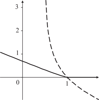
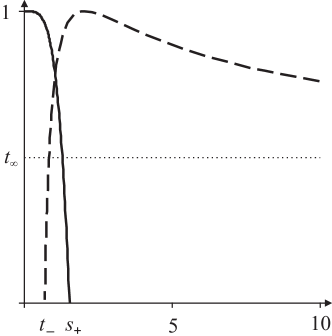
Figure 5.1. Infinite critical value ${p(t_{\infty})=\infty}$ and no phase transition for the $\alpha_{H}$-Farey free energy function and the $\alpha_{H}$-Lüroth pressure function. The figure shows the $\alpha_{H}$-Farey free energy $v$ (solid line), the $\alpha_{H}$-Lüroth pressure function $p$ (dashed line), and the associated dimension graphs $\sigma_{\alpha}$ and $\tau_{\alpha}$ of the alternating Lüroth system. Here, $t_{-}=\log 2,t_{\infty}=1/2$ and $s_{+}=(\log 6)/2$. Both $F_{\alpha_{H}}$ and $L_{\alpha_{H}}$ experience no phase transition.

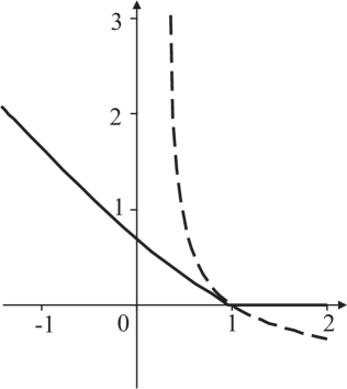
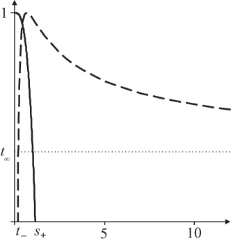
Figure 5.2. Phase transition for the $\alpha$-Farey free energy function, no phase transition for the the $\alpha$-Lüroth pressure function and $\alpha$ expansive. The $\alpha$-Farey free energy $v$ (solid line), the $\alpha$-Lüroth pressure function $p$ (dashed line), and the associated dimension graphs for $a_{n}:=\zeta\left(3\right)^{-1}n^{-3}$. Here, $F_{\alpha}$ has a phase transition, namely, $p$ is not differentiable at $1$, whereas $L_{\alpha}$ exhibits no phase transition and ${p(t_{\infty})=\infty}$.

Note that the Hölder exponent of the map $\theta_{\alpha_{H}}$ is equal to $2\log 2/\log 6$. Also, it is immediately clear that the invariant measure $\nu_{\alpha_{H}}$ associated to $F_{\alpha_{H}}$ is infinite, and that the density function of $\nu_{\alpha_{H}}$ with respect to $\lambda$ is equal to the step function $\sum_{n=1}^{\infty}(n+1)\mathbbm{1}_{A_{n}}$.

Remark. Suppose that in the definition of $F_{\alpha_{H}}$ given above we were to choose $x\mapsto 2x-1$ instead of $x\mapsto 2-2x$ for the right-hand branch of the $\alpha_{H}$-Farey map, with $1/2\mapsto 0$. Then, the jump transformation of this new non-alternating version of $F_{\alpha_{H}}$ coincides with the actual classical Lüroth map ${L}:\mathcal{U}\to\mathcal{U}$, which generates the series expansion of real numbers introduced by Lüroth in [22] and which is given in our terms by

$$L(x)=\left\{\begin{array}[]{ll}n(n+1)x-n,&\text{ for }x\in[1/(n+1),1/n),\ n\geq 2;\\ 2x-1,&\hbox{ for $x\in[1/2,1]$.}\\ 0,&\hbox{ for $x=0$.}\end{array}\right.$$

The series expansion in this case is given by

$$x=\sum_{n=1}^{\infty}\left(\ell_{n}\prod_{k=1}^{n}(\ell_{k}(\ell_{k}+1))^{-1}\right),$$

where again all of the $\ell_{i}$ are natural numbers. Notice that the atoms of the partition behind the map $L$ are slightly different to the atoms $A_{n}$ of $\alpha_{H}$, they are right closed and left open intervals, except for the equivalent of $A_{1}$, which is the closed interval $[1/2,1]$.

We now consider the $\alpha_{H}$-sum-level sets. The reader might like to see that the Lebesgue measures of the first members of the sequence $\left(\mathcal{L}^{(\alpha_{H})}_{n}\right)$ are as follows:

$$\lambda(\mathcal{L}^{(\alpha_{H})}_{0})=1,\;\lambda(\mathcal{L}^{(\alpha_{H})}_{1})=\frac{1}{2},\;\lambda(\mathcal{L}^{(\alpha_{H})}_{2})=\frac{5}{12},\;\lambda(\mathcal{L}^{(\alpha_{H})}_{3})=\frac{3}{8},\;\lambda(\mathcal{L}^{(\alpha_{H})}_{4})=\frac{251}{720}.$$

Since the Lebesgue measure of the sum-level set $\mathcal{L}_{n}$ associated with the map $L$ coincides with the Lebesgue measure of the sum-level set ${\mathcal{L}}^{(\alpha_{H})}_{n}$, Theorem 1 gives the following corollaries.

Corollary 5.1.

$\displaystyle{\lim_{n\to\infty}\lambda\left(\mathcal{L}^{(\alpha_{H})}_{n}\right)=\lim_{n\to\infty}\lambda\left(\mathcal{L}_{n}\right)=0}$.

Corollary 5.2.

For the classical and for the alternating Lüroth map the following hold, for $n$ tending to infinity.

1. $\displaystyle{\sum_{k=1}^{n}\lambda\left(\mathcal{L}_{n}\right)=\sum_{k=1}^{n}\lambda\left({\mathcal{L}}_{n}^{(\alpha_{H})}\right)\sim n\left(\sum_{k=1}^{n}\frac{1}{k}\right)^{-1}\sim\frac{n}{\log n}}$;

2. $\displaystyle{\lambda\left(\mathcal{L}_{n}\right)=\lambda\left({\mathcal{L}}_{n}^{(\alpha_{H})}\right)\sim\left(\sum_{k=1}^{n}\frac{1}{k}\right)^{-1}\sim\frac{1}{\log n}}$.

For the outcome of the Lyapunov spectra associated with the harmonic partition we refer to Fig. 5.1. Also, various different phenomena which arise from particularly chosen partitions are briefly discussed in Fig. 5.2, 5.3, 5.4, 5.5, 5.6 (see also Remark 2 in the introduction).

References

- [1] J. Aaronson. An introduction to infinite ergodic theory, volume 50 of Mathematical Surveys and Monographs. American Mathematical Society, Providence, RI, 1997.
- [2] J. Aaronson, M. Denker, M. Urbański. Ergodic theory for Markov fibred systems and parabolic rational maps. Trans. Amer. Math. Soc. 33(2):495-548, 1993.
- [3] J. Barrionuevo, R. M. Burton, K. Dajani and C. Kraaikamp. Ergodic properties of generalised Lüroth series. Acta Arith., LXXIV (4), 311-327, 1996.
- [4] N. H. Bingham, C. M. Goldie, J. L. Teugels. Regular variation, Volume 27 of Encyclopedia of Mathematics and its Applications. Cambridge University Press, Cambridge, 1989.
- [5] K. Dajani, C. Kraaikamp. On approximation by Lüroth series. J. Théor. Nombres Bordeaux, 8:331–346, 1996.
- [6] K. Dajani, C. Kraaikamp. Ergodic theory and numbers. Carus Math. Monogr. 29. Math. Assoc. of America, Washington, DC, 2002.
- [7] J. L. Doob. Stochastic processes. Wiley, New York, 1953.
- [8] P. Erdős, H. Pollard, W. Feller. A property of power series with positive coefficients. Bull. Amer. Math. Soc. 55:201-204, 1949.
- [9] K. B. Erickson. Strong renewal theorems with infinite mean. Trans. Amer. Math. Soc. 151:263-291, 1970.
- [10] A. Garsia, J. Lamperti. A discrete renewal theorem with infinite mean. Comment. Math. Helv. 37:221–234, 1963.
- [11] K. Gelfert, M. Rams. The Lyapunov spectrum of some parabolic systems. Ergodic Theory Dynam. Systems 29(3):919–940, 2009.
- [12] I. J. Good. The fractional dimensional theory of continued fractions. Proc. Cambridge Phil. Soc. 37, 199–228, 1941.
- [13] E. Hopf. Ergodentheorie. Ergeb. Mat., Vol. 5, Springer, 1937.
- [14] J. Jaerisch, M. Kesseböhmer. Regularity of multifractal spectra of conformal iterated function systems. Trans. Amer. Math. Soc. 363(1):313–330, 2011.
- [15] S. Kalpazidou, A. Knopfmacher and J. Knopfmacher. Metric properties of alternating Lüroth series. Portugal. Math. 48:319–325, 1991.
- [16] M. Kesseböhmer, B.O. Stratmann. A multifractal analysis for Stern-Brocot intervals, continued fractions and Diophantine growth rates. J. Reine Angew. Math. 605:133–163, 2007.
- [17] M. Kesseböhmer, B.O. Stratmann. Fractal analysis for sets of non-differentiability of Minkowski’s question mark function. J. Number Theory 128:2663–2686, 2008.
- [18] M. Kesseböhmer, B.O. Stratmann. On the Lebesgue measure of sum-level sets for continued fractions. To appear in Discrete Contin. Dyn. Syst.
- [19] A. N. Kolmogorov. Foundations of the theory of probability. Chelsea, New York, 1956.
- [20] U. Krengel. Ergodic Theorems. De Gruyter, Berlin, 1985.
- [21] M. Lin. Mixing for Markov operators. Z. Wahrsch. Verw. Gebiete 19:231–243, 1971.
- [22] J. Lüroth. Über eine eindeutige Entwicklung von Zahlen in eine unendliche Reihe. Math. Ann. 21:411–423, 1883.
- [23] H. Minkowski. Geometrie der Zahlen. Gesammelte Abhandlungen, Vol. 2, 1911; reprinted by Chelsea, New York, 43–52, 1967.
- [24] S. Munday. A note on Diophantine-type fractals for -Lüroth systems. Preprint in: arXiv:1011.5391, 2010.
- [25] R. Salem. On some singular monotonic functions which are strictly increasing. Trans. Amer. Math. Soc. 53(3):427–439, 1943.
- [26] O. Sarig. Phase transitions for countable Markov shifts. Comm. Math. Phys. 217(3):555–577, 2001.
- [27] X.-J. Wang. Statistical physics of temporal intermittency. Physical Review A 40(11):6647–6661, 1989.