Modeling the Radial Velocities of HD 240210 with the Genetic Algorithms

Abstract

More than 450 extrasolar planets are known to date. To detect these intriguing objects, many photometric and radial velocity (RV) surveys are in progress. We developed the Keplerian FITting (KFIT) code, to model published and available RV data. KFIT is based on a hybrid, quasi-global optimization technique relying on the Genetic Algorithms and simplex algorithm. Here, we re-analyse the RV data of evolved K3III star HD 240210. We confirm three equally good solutions which might be interpreted as signals of 2-planet systems. Remarkably, one of these best-fits describes long-term stable two-planet system, involved in the 2:1 mean motion resonance (MMR). It may be the first instance of this strong MMR in a multi-planet system hosted by evolved star, as the 2:1 MMR configurations are already found around a few solar dwarfs.

¹Toruń Centre for Astronomy, Nicolaus Copernicus University, Gagarin Str. 11, 87-100 Toruń, Poland
{a.rozenkiewicz,k.gozdziewski,c.migaszewski}@astri.umk.pl

Introduction

Most of the discovered exoplanets are found around main sequence stars, perhaps because the determination of stellar parameters is much easier than, for instance for giant or active stars. The formation theory of planets hosted by such stars is still developed and not understood well. Recently, there are only known about of 10 exoplanets orbiting stars with masses greater than 2 $M_{\odot}$ (see, e.g., Extrasolar Planets Encyclopaedia, http://exoplanet.eu). Some recent RV surveys focus on detecting planets around the red giants, which are evolved main sequence stars. Unfortunately, the giants and sub-giants are difficult targets for the RV technique. Usually, they are chromospherically active, pulsating, surface-polluted by large spots, and rotating slowly. The giants produce small number of sharp spectral lines and their chromospheric activity and spots may change the profiles of spectral lines. This intrinsic RV variability (also known as stellar ”jitter”) is significantly larger than instrumental errors, and may be $\sim 20-30$ m/s and larger. Actually, the stellar activity may even mimic planetary signals (see, e.g. [1]). Hence, when interpreting the RV variability, we may expect that different uncertainties and errors (usually, of unknown origin) may significantly shift the best fits from the “true” solutions in the parameters space. In such a case, possibly global exploration of the parameter space and the dynamical stability of multiple systems as an additional, implicit observable may help us to correct and verify the derived best-fit solutions for these factors, and to conclude on the architecture of interacting systems, even when limited data are available [4].

Keplerian model of the RV and optimization method

We recall the kinematic RV model for the $N$-planet system, as the first order approximation of the $N$-body model:

$$V_{r}(t)=\sum_{i=1}^{N}K_{i}\left[\cos(\omega_{i}+\nu(t))+e_{i}\cos(\omega_{i})\right]+V_{0},$$ (1)

where, for each planet in the system, $K_{i}$ is the semi-amplitude of the signal, $e_{i}$ is the orbital eccentricity, $\omega_{i}$ is the argument of pericenter, $\nu_{i}(t)$ is the true anomaly, which depends on the orbital period $P_{i}$, the time of periastron passage $\tau_{i}$ and eccentricity, and $V_{0}$ is a constant instrumental offset. The $N$-planet system is then characterized by $N_{p}=5N+1$ free parameters, to be determined from observations. Let us note, that the inclinations and longitudes of nodes are not explicitly present in Eq. (1) and cannot be determined directly from the RV data alone, at least in terms of the kinematic model in Eq. (1).

To fit model Eq. (1) to the RV data, the Gaussian Least-Squares method is commonly used. To estimate the best-fit model parameters, we seek for the minimum of the reduced $\chi^{2}$ function, $\min\sqrt{\chi^{2}_{\nu}}({\bf p})$, which is computed on the basis of synthetic signal $V_{r}(t_{i},{\bf p})$, where $t_{i}$ are moments of observations $V_{r,i}^{obs}$ with uncertainties $\sigma_{i}$ ($i=1,\ldots,N_{RV}$ is the number of data), and ${\bf p}\equiv(K_{p},P_{p},e_{p},\omega_{p},\tau_{p},V_{0})$, and $p=1\equiv b,2\equiv c,\ldots,N$ are for the model parameters of the $N$-planet system.

Clearly, even in the kinematic formulation, $\sqrt{\chi^{2}_{\nu}}({\bf p})$ is a non-linear function. It is well known that it may exhibit numerous local extrema. Hence, the exploration of multi-dimensional parameter space ${\bf p}$ requires efficient, possibly global numerical optimization. In the past, we found that good results in this problem may be achieved by an application of the Genetic Algorithms (GAs) [2], which mimic the biological evolution. GAs search for the best fit solutions (best adapted population members) to the model (to the environment) through “breading” an initial population (parameters set), under particular genetic operators (e.g., cross-over, mutation), and through a selection of gradually better adapted members. Although the GAs start with purely random initial “population”, the search converges to the best fit solutions [2] by deterministic way. Of course, the best fit solutions may be not unique. This is very common in the case of modeling RV data. Overall, the GAs are robust and quasi-global optimization technique, although they not provide efficiency and accuracy of fast local methods, like the Levenberg-Marquardt algorithm. The GAs are used in our hybrid KFIT code, developed for a few years now [3], which also makes use of the local, and accurate simplex algorithm [6]. It helps to quickly refine the final population of the best fits, “grown” by the GAs.

The results for the RV of HD 240210

In a recent work, Niedzielski et al. [5] detected a planet hosted by evolved dwarf HD 240210. They found an excess in the rms of Keplerian 1-planet model, and interpret this as possible signal of an additional planet. We reproduced their 1-planet solution, see Fig. 1 (the top-left panel). The rms has significant scatter of $39$ m/s, compared to the mean instrumental accuracy of $\sim 8$ m/s. This rms excess is difficult to explain by the internal variability of the star, hence we tried to find a better 2-planet model. At first, we reproduced (see Fig. 1, the top-right panel) a tentative 2-planet solution illustrated in the discovery paper. However, we notice that the orbital periods are very similar $\sim 440$ and $\sim 530$ days, respectively, indicating strong 4:3 MMR or 1:1 MMR. In such a case, the kinematic model is not proper anymore, due to significant mutual planetary interactions. Moreover, such configurations could be hardly explained by the planetary formation theory.

Figure 1: The RV observations of HD 240210 [5] and synthetic curves for the best fit solutions found in this paper. The left-upper panel: the best 1-planet fit. Subsequent figures are for the best fits labeled with I, II, III in Fig. 2. For a reference, all these plots are accompanied by the model curve of the 1-planet fit. See Table 1 for orbital elements.

Still, having in mind that this solution is not unique, we performed an extensive search for the local minima of $\sqrt{\chi^{2}_{\nu}}$ with the KFIT code. The statistics of gathered fits is shown in Fig. 2, through their projection onto orbital periods plane. In the range of orbital periods $\in[60,3600]$ days, we found three, equally good best-fit models, which correspond to different orbital configurations, and may be resolved at the $2\sigma$ confidence level. In the parameter maps, the mentioned 2-planet model is labeled as Fit I. Two additional fits with orbital periods ratio close to 3:2 and 2:1 are labeled as Fit II and Fit III, respectively (see Table 1). Their synthetic RV curves, with the RV of 1-planet model (thin curve) and observations overplotted, are shown in subsequent panels of Fig. 1. Note, that the alternative 2-planet fits reduce the rms significantly, to $\sim 25$ m/s (i.e., by 1/3), consistent with a conclusion in [5].

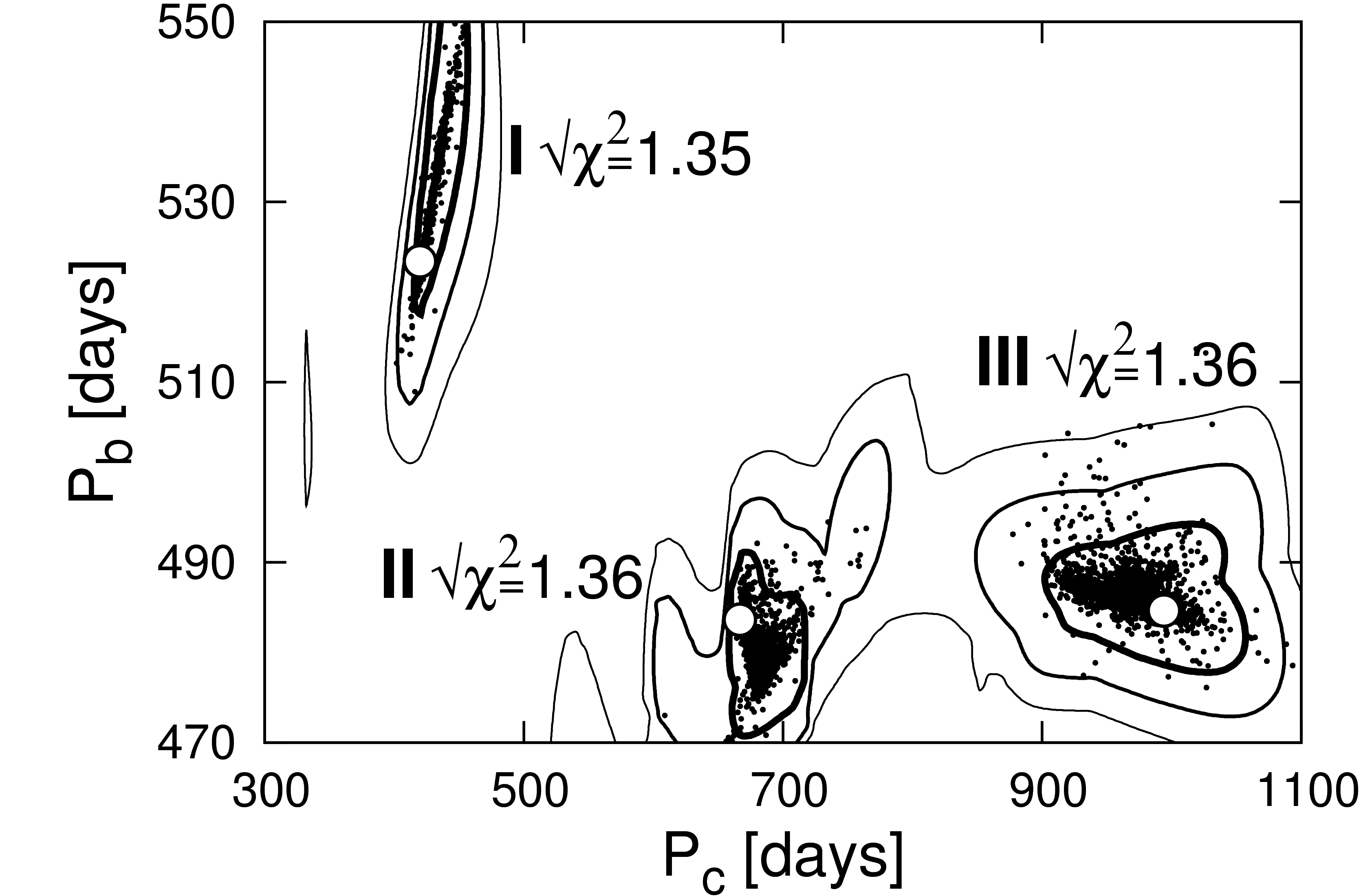
Figure 2: Statistics of the Keplerian best fits gathered with the KFIT code, projected onto the ($P_{b}$, $P_{c}$)–plane of orbital periods. Solutions marked with white circles and labeled by I, II, III are for the best fits in different “islands” of the parameters space. Black filled circles are for all fits within formal 3$\sigma$-level of Fit I; for a reference contours with 3,2,1 $\sigma$-level of this solution, found through extensive, systematic scanning [4] of the ($P_{b}$, $P_{c}$)-plane with the Levenberg-Marquardt algorithm, are plotted as curves of increasing thickness. See Table 1 for model parameters.

As may be seen in Table 1, Fits II and III have large eccentricities. A question remains, whether inferred orbital configurations are dynamically stable. In fact, all these Fits I–III, transformed to osculating elements at the epoch of the first observation, lead to self-disruption of 2-planet systems. Nevertheless, remembering that stable solutions may still be found in their neighborhood, we did dynamical analysis with the $N$-body, self-consistent GAMP code [4] (which also relies on the GAs), trying to refine Fits I–III with the requirement of the long-term stability (the edge-on, coplanar models are tested). Certainly, at most one of these models might correspond to the real system. We did not found any stable orbits in the vicinity of Fit I. In a tiny neighborhood of Fit II, there is a stable configuration with $\sqrt{\chi^{2}_{\nu}}\sim 1.50$ and an rms $\sim 27$ m/s which, as the direct numerical integrations show, is stable over 1 Gyr. The best result is found for Fit III as a stable solution, corresponding to the 2:1 MMR with $\sqrt{\chi^{2}_{\nu}}\sim 1.36$ and an rms of $\sim 25$ m/s, i.e., the same as in the kinematic Fit III. The dynamical map [4] around this solution (Fig. 3, the right-hand panel) reveals extended island of stability ($\sim 0.15$ au). This fit has moderate semi-amplitude librations ($\sim 15-30^{\circ}$) of the critical angles $\theta_{1}=2\lambda_{b}-\lambda_{c}-\varpi_{b}$ (around $0^{\circ}$), $\theta_{2}=2\lambda_{b}-\lambda_{c}-\varpi_{c}$ (around $180^{\circ}$), and $\theta_{3}=\varpi_{b}-\varpi_{c}$ (around $180^{\circ}$). The numerical integrations confirmed that its stability is preserved at least over 1 Gyr.

 

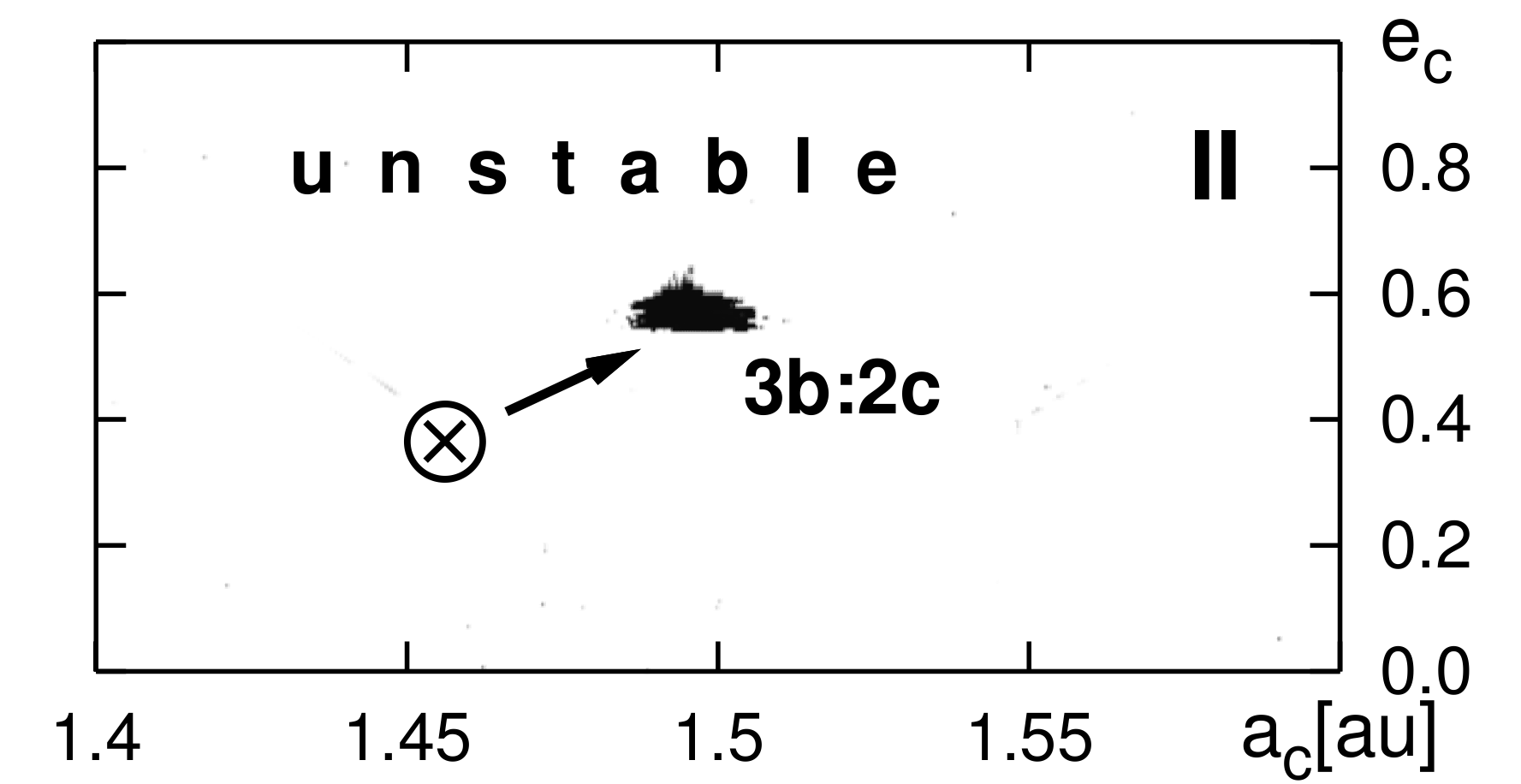
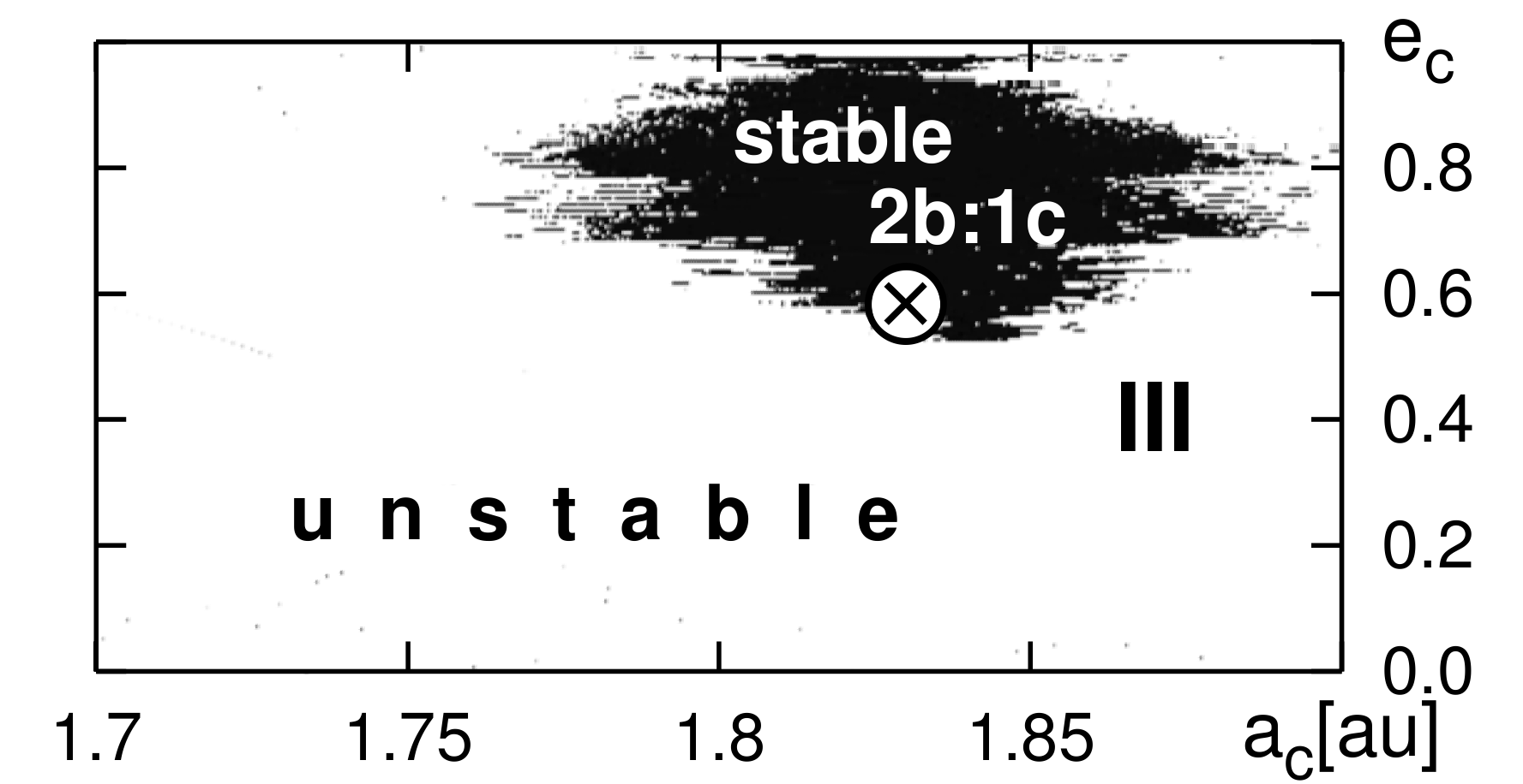
Figure 3: Dynamical maps in terms of the MEGNO indicator [4] around coplanar, edge-on, GAMP $N$-body fits (crossed circle): Fit II (3:2 MMR, $\sqrt{\chi^{2}_{\nu}}=1.50$, rms $\sim 27$ m/s, the left-hand panel), and Fit III (2:1 MMR, $\sqrt{\chi^{2}_{\nu}}=1.36$, rms $\sim 25$ m/s, the right-hand panel). White color is for unstable configurations, black is for stable solutions. Orbits at the epoch of the first RV of Fit III in terms of $(m\,\mbox{[m}_{J}\mbox{]},a\,\mbox{[au]},e,\omega\,\mbox{[deg]},{\cal M}\,\mbox{[deg]})$ are the following: (4.11, 1.14, 0.284, 304.8, 101.8)_b, (2.27, 1.83, 0.592, 162.3, 304.2)_c for planets b, and c, respectively, $V_{0}=21.57$ m/s, stellar mass is 0.82 M_⊙ [5]; Fit II is: (4.50, 1.143, 0.217, 249.24, 163.87)_b, (1.94, 1.506, 0.562, 53.09, 243.39)_c, $V_{0}=8.98$ m/s.

The 2:1 MMR Fit III seems the most promising planetary model explaining the RV variability of the HD 240210. The 2:1 MMR is quite frequent in the sample of $\sim 40$ known extrasolar systems with jovian planets, because 5–6 configurations were reported (see, http://exoplanet.eu). Hence, this new system, which could be the first one around evolved star, is likely. We stress that solution III is found in relatively extended stability zone, unlike Fit II, which lies in a tiny, isolated area ($\sim 0.01$ au, Fig.3, the left-hand panel). These two maps almost overlap in the $a_{c}$-range, hence other, relatively extended stable islands are rather excluded in this region.

Table 1: Keplerian model parameters of 2-planet best fit solutions to the RV of HD 240210. Formal measurement errors are rescaled by adding the stellar jitter of $\sigma_{j}=20$ m/s in quadrature. $T_{0}\equiv 53,000$ days, $N_{v}=N_{RV}-N_{p}=27$.

the best fit	I		II		III
parameters	b	c	b	c	b	c
$P$ [day]	540 $\pm$ 29	441 $\pm$ 27	484 $\pm$ 14	667 $\pm$ 54	485 $\pm$ 18	994 $\pm$ 97
$K$ [m/s]	131 $\pm$ 29	85 $\pm$ 30	147 $\pm$ 16	82 $\pm$ 36	129 $\pm$ 30	63 $\pm$ 23
$e$	0.05 $\pm$ 0.09	0.20 $\pm$ 0.14	0.18 $\pm$ 0.14	0.74 $\pm$ 0.38	0.30 $\pm$ 0.13	0.58 $\pm$ 0.35
$\omega$ [deg]	204 $\pm$ 51	356 $\pm$ 73	261 $\pm$ 41	36 $\pm$ 76	302 $\pm$ 35	163 $\pm$ 87
$\tau-T_{0}$ [days]	352 $\pm$ 65	610 $\pm$ 109	484 $\pm$ 45	502 $\pm$ 72	536 $\pm$ 31	326 $\pm$ 156
$V_{0}$[m/s]	-3$\pm$7		12 $\pm$ 9		22$\pm$ 12
$\sqrt{\chi^{2}_{\nu}}$	1.35		1.36		1.36
rms [m/s]	25.2		25.2		25.2

Conclusions

Extrasolar planets hosted by giant or evolved stars bring important border conditions for the planet formation theory. In this work, we re-analysed the literature RV data for evolved dwarf HD 240210, with our KFIT code relying on quasi-global GAs. In the reasonable range of orbital periods less than 3600 days, we found three Keplerian solutions, which have the same $\sqrt{\chi^{2}_{\nu}}$ and an rms. By further dynamical analysis of these best-fit models, we selected the most likely, stable solution, which corresponds to 2:1 MMR, and is located in relatively extend zone of dynamical stability. Overall, if the 2-planet configuration is assumed, the dynamical constraints seem rule out other two models, but only new observations may confirm the 2:1 MMR hypothesis.

Acknowledgements. This work is supported by Polish Ministry of Science, Grant 92/N-ASTROSIM/2008/0.

References

- [1] Berdyugina, S. V., LRSP, 2(8) (1995)
- [2] Charbonneau, P., ApJS, 101, 309 (1995)
- [3] Goździewski K., Migaszewski, C., A&A, 449, pp.1219-1232 (2006)
- [4] Goździewski K., Migaszewski & C., Musieliński, A., Proc. IAU Symp. 249, pp.1219-1232 (2008)
- [5] Niedzielski A., Nowak G., Adamów M. & Wolszczan A., ApJ, 707, pp. 768-777 (2009)
- [6] Nelder J. A., Mead R., Comp. J., 7, pp. 308-313 (1965)