High-energy amplitudes and impact factors at next-to-leading order

Abstract:

To study scattering amplitudes at high-energy, the T-product of two currents can be expanded in terms of coefficient functions (impact factors) and matrix elements of “composite color dipoles” made of Wilson line operators with rapidity cutoff preserving conformal invariance. In the leading order, the high-energy evolution of color dipoles is governed by the non-linear Balitsky-Kovchegov (BK) equation. To describe the high-energy amplitudes in the next-to-leading order (NLO) one needs to know the coefficient function (“impact factor”) and the evolution of corresponding Wilson-line operators. Using the high-energy OPE, we find the next-to-leading order (NLO) correction to the BK equation and calculate the impact factor for virtual photons in deep inelastic scattering.

1 Introduction

Wilson line operators are the effective degrees of freedom for the description of high-energy scattering in gauge theories (for a review, see Ref. [1, 2]). Indeed, at high-energy (Regge limit) particles move along their straight-line classical trajectory and the only quantum effect is the eikonal phase factor acquired along this propagation path. In QCD, for fast quarks or gluons scattering off some target, this eikonal phase factor is a Wilson line - an infinite gauge link ordered along the straight line collinear to particle’s velocity $n^{\mu}$:

$$U^{\eta}(x_{\perp})={\rm Pexp}\Big{\{}ig\int_{-\infty}^{\infty}\!\!du~{}n_{\mu}~{}A^{\mu}(un+x_{\perp})\Big{\}}~{}~{}~{}~{}$$ (1)

where $A_{\mu}$ is the gluon field of the target, $x_{\perp}$ is the transverse position of the particle which remains unchanged throughout the collision, and the index $\eta$ is the rapidity of the particle. The high-energy behavior of QCD amplitudes can then be studied in the framework of the evolution of color dipoles. We consider the small-x behavior of structure functions of deep inelastic scattering (DIS): the virtual photon decomposes into quark and antiquark pair which propagate along the straight lines separated by transverse distance and forms a color dipole - two-Wilson-line operator:

$$\hat{\cal U}^{\eta}(x_{\perp},y_{\perp})=1-{1\over N_{c}}{\rm tr}\{\hat{U}^{\eta}(x_{\perp})\hat{U}^{\dagger\eta}(y_{\perp})\}$$ (2)

The energy dependence of the structure function is translated into the dependence of the color dipole on the rapidity $\eta$. Although it appears to be more natural to restrict the rapidity by considering the Wilson line with the supporting line collinear to the velocity of the fast-moving particle, we choose to cut the rapidity integrals “by hand”: the method of “rigid cutoff” in the longitudinal direction is technically simpler and more efficient in order to get the conformal results. Thus, the small-x behavior of the structure functions is governed by the rapidity evolution of color dipoles [3, 4]. At relatively high energies and for sufficiently small dipoles we can use the leading logarithmic approximation (LLA) where $\alpha_{s}\ll 1,~{}\alpha_{s}\ln x_{B}\sim 1$ and get the non-linear BK evolution equation for the color dipoles [6, 7]:

$${d\over d\eta}~{}\hat{\cal U}^{\eta}(z_{1},z_{2})~{}=~{}{\alpha_{s}N_{c}\over 2\pi^{2}}\!\int\!d^{2}z_{3}~{}{z_{12}^{2}\over z_{13}^{2}z_{23}^{2}}[\hat{\cal U}^{\eta}(z_{1},z_{3})+\hat{\cal U}^{\eta}(z_{3},z_{2}))$$

$$\hskip 85.35826pt-\hat{\cal U}^{\eta}(z_{1},z_{3})-\hat{\cal U}^{\eta}(z_{1},z_{3})\hat{\cal U}^{\eta}(z_{3},z_{2})]$$ (3)

where $\eta=\ln{1\over x_{B}}$ and $z_{12}\equiv z_{1}-z_{2}$ etc. (we denote operators by “hat”). The first three terms in the BK equation correspond to the linear BFKL evolution [5] and describe the partons emission while the last term is responsible for the partons annihilation. For sufficiently low $x_{B}$ the partons emission balances the partons annihilation so the partons reach the state of saturation [8] with the characteristic transverse momentum $Q_{s}$ growing with energy $1/x_{B}$ (for a review, see [9]).

2 Next-to-leading order photon impact factor

In the Regge limit all transverse momenta are of the same order of magnitude and consequently it is natural to introduce a factorization scale in rapidity: one introduces a rapidity divide $\eta$ which separate “fast” field from “slow” fields. Thus, the amplitude of the process is given by a convolution of contributions coming from fields with rapidity $\eta<Y$ (“fast” field) and contributions coming from fields with rapidity $\eta>Y$ (“slow” fields). As in the case of the usual Operator Product Expansion (OPE), the integration over the field with rapidity $\eta<Y$ gives us the coefficients function while the integrations over the field with rapidity $\eta>Y$ are the matrix elements of the operators. Thus, the OPE at high-energy (Regge limit) for the T-product of two electromagnetic currents is obtained in terms of Wilson lines

$$T\{\hat{j}_{\mu}(x)\hat{j}_{\nu}(y)\}=\int\!d^{2}z_{1}d^{2}z_{2}~{}I^{\rm LO}_{\mu\nu}(z_{1},z_{2})[{\rm Tr}\{\hat{U}^{\eta}_{z_{1}}\hat{U}^{\dagger\eta}_{z_{2}}\}]^{\rm conf}$$

$$+\int\!d^{2}z_{1}d^{2}z_{2}d^{2}z_{3}~{}I^{\rm NLO}_{\mu\nu}(z_{1},z_{2},z_{3})[{\rm tr}\{\hat{U}^{\eta}_{z_{1}}\hat{U}^{\dagger\eta}_{z_{3}}\}{\rm tr}\{\hat{U}^{\eta}_{z_{3}}\hat{U}^{\dagger\eta}_{z_{2}}\}-N_{c}{\rm tr}\{\hat{U}^{\eta}_{z_{1}}\hat{U}^{\dagger\eta}_{z_{2}}\}]$$ (4)

where

$$[{\rm Tr}\{\hat{U}^{\eta}_{z_{1}}\hat{U}^{\dagger\eta}_{z_{2}}\}\big{]}^{\rm conf}={\rm Tr}\{\hat{U}^{\eta}_{z_{1}}\hat{U}^{\dagger\eta}_{z_{2}}\}$$

$$+{\alpha_{s}\over 2\pi^{2}}\!\int\!d^{2}z_{3}~{}{z_{12}^{2}\over z_{13}^{2}z_{23}^{2}}[{\rm Tr}\{T^{n}\hat{U}^{\eta}_{z_{1}}\hat{U}^{\dagger\eta}_{z_{3}}T^{n}\hat{U}^{\eta}_{z_{3}}\hat{U}^{\dagger\eta}_{z_{2}}\}-N_{c}{\rm Tr}\{\hat{U}^{\eta}_{z_{1}}\hat{U}^{\dagger\eta}_{z_{2}}\}]\ln{az_{12}^{2}\over z_{13}^{2}z_{23}^{2}}$$ (5)

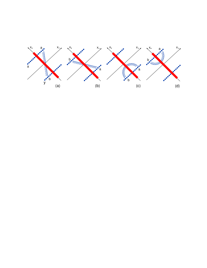
Figure 1: Leading-order diagrams for the small-$x$ evolution of color dipole. Wilson lines are denoted by dotted lines.

is the composite dipole with the conformal longitudinal cutoff in the next-to-leading order. The appearance of the composite operators is due to the loss of conformal invariance of the Wilson line operator in the NLO. Indeed, the light-like Wilson lines $U(x_{\perp})$ are formally Möbius invariant and consequently the leading-order BK equation is also conformal invariant. At NLO the Wilson line operator are divergent and its regularization introduces a dependence on the rapidity and conformal symmetry is lost. In order to restore the conformal invariance we redefine the operator ${\rm Tr}\{\hat{U}^{\eta}_{z_{1}}\hat{U}^{\dagger\eta}_{z_{2}}\}$ by adding suitable conterterms. The procedure of finding the dipole with conformally regularized rapidity divergence is analogous to the construction of the composite renormalized local operator by adding the appropriate counterterms order by order in perturbation theory. In equation (4) the coefficient $I^{\rm LO}$ is the leading-order (LO) impact factor which has been known for long time, while $I^{\rm NLO}$ is the NLO impact factor [15] given by

$$I^{NLO}_{\mu\nu}(x,y)=-{\alpha_{s}N_{c}^{2}\over 8\pi^{7}x_{*}^{2}y_{*}^{2}}\!\int\!d^{2}z_{1}d^{2}z_{2}~{}{\cal U}^{\rm conf}(z_{1},z_{2})\Bigg{\{}\Bigg{[}{1\over{\cal Z}_{1}^{2}{\cal Z}_{2}^{2}}\partial^{x}_{\mu}\partial^{y}_{\nu}\ln{\Delta^{2}\over x_{\ast}y_{\ast}}$$ (6)

$$+~{}2{\big{(}\partial_{\mu}^{x}{\cal Z}_{1}\big{)}\big{(}{\cal Z}_{2}\partial_{\nu}^{y}\big{)}\over{\cal Z}_{1}^{3}{\cal Z}_{1}^{3}}\big{[}\ln{1\over R}+{1\over 2R}-2\big{]}+~{}{2\big{(}\partial^{x}_{\mu}{\cal Z}_{1}\big{)}\big{(}\partial^{y}_{\nu}{\cal Z}_{1}\big{)}\over{\cal Z}_{1}^{4}{\cal Z}_{2}^{2}}\big{[}\ln{1\over R}-{1\over 2R}\big{]}$$

$$-~{}{1\over 2}\Big{[}{\partial^{x}_{\mu}{\cal Z}_{1}\over{\cal Z}_{1}^{3}{\cal Z}_{2}^{2}}\partial^{y}_{\nu}\ln{\Delta^{2}\over x_{\ast}y_{\ast}}+{\partial^{y}_{\nu}{\cal Z}_{1}\over{\cal Z}_{1}^{3}{\cal Z}_{2}^{2}}\partial^{x}_{\mu}\ln{\Delta^{2}\over x_{\ast}y_{\ast}}\Big{]}\big{(}1-{1\over R}\big{)}-{1\over 2{\cal Z}_{2}^{2}}\Big{[}\big{(}\partial^{x}_{\mu}{1\over{\cal Z}_{1}^{2}}\big{)}\partial^{y}_{\nu}R+\big{(}\partial^{y}_{\nu}{1\over{\cal Z}_{1}^{2}}\big{)}\partial^{x}_{\mu}R\Big{]}{\ln R\over 1-R}$$

$$-~{}\big{(}\partial^{x}_{\mu}\partial^{y}_{\nu}{\Delta^{2}\over x_{\ast}y_{\ast}}\big{)}{R^{3}\over z_{12}^{4}}\big{[}{1\over R}+{3\over 2R^{2}}-2\big{]}\big{(}{x_{\ast}y_{\ast}\over\Delta^{2}}\big{)}^{3}+{1\over R}\Big{[}{\partial^{x}_{\mu}{\cal Z}_{1}\over{\cal Z}_{1}^{3}{\cal Z}^{2}_{2}}\big{(}\partial^{y}_{\nu}\ln{\Delta^{2}\over x_{\ast}y_{\ast}}\big{)}+{\partial^{y}_{\nu}{\cal Z}_{1}\over{\cal Z}_{1}^{3}{\cal Z}^{2}_{2}}\big{(}\partial^{x}_{\mu}\ln{\Delta^{2}\over x_{\ast}y_{\ast}}\big{)}\Big{]}$$

$$+~{}4{\big{(}\partial^{x}_{\mu}{\cal Z}_{1}\big{)}\big{(}\partial^{y}_{\nu}{\cal Z}_{2}\big{)}\over{\cal Z}_{1}^{3}{\cal Z}_{2}^{3}}\Big{[}4{\rm Li}_{2}(1-R)-{2\pi^{2}\over 3}+2(\ln R-1)\big{(}\ln R-{1\over R}\big{)}\Big{]}$$

$$+~{}2{\big{(}\partial^{x}_{\mu}{\cal Z}_{1}\big{)}\big{(}\partial^{y}_{\nu}{\cal Z}_{2}\big{)}\over{\cal Z}_{1}^{3}{\cal Z}_{2}^{3}}\Big{[}{\ln R\over R(1-R)}-{1\over R}+2\ln R-4\Big{]}+2{\big{(}\partial^{x}_{\mu}{\cal Z}_{1}\big{)}\big{(}\partial^{y}_{\nu}{\cal Z}_{1}\big{)}\over{\cal Z}_{1}^{4}{\cal Z}_{2}^{2}}\Big{[}{\ln R\over R(1-R)}-{1\over R}\big{]}$$

$$-\Big{(}{\partial^{x}_{\mu}{\cal Z}_{1}\over{\cal Z}_{1}^{3}{\cal Z}_{2}^{2}}\partial^{y}_{\nu}\ln{\Delta^{2}\over x_{*}y_{*}}+{\partial^{y}_{\nu}{\cal Z}_{2}\over{\cal Z}_{2}^{3}{\cal Z}_{1}^{2}}\partial^{x}_{\mu}\ln{\Delta^{2}\over x_{*}y_{*}}\Big{)}\Big{[}{\ln R\over R(1-R)}-2\Big{]}+~{}(z_{1}\leftrightarrow z_{2})\Bigg{]}$$

$$-~{}2{z_{12\perp}^{2}\over{\cal Z}_{1}^{3}{\cal Z}_{2}^{3}}\Big{[}4{\rm Li}_{2}(1-R)-{2\pi^{2}\over 3}+2(\ln{1\over R}+{1\over R}+{1\over 2R^{2}}-3)\ln{1\over R}-\big{(}6+{1\over R}\big{)}\ln R+{3\over R}-4\Big{]}\partial^{x}_{\mu}\partial^{y}_{\nu}{\Delta^{2}\over x_{\ast}y_{\ast}}\Bigg{\}}$$

where

$$\Delta\equiv(x-y),~{}~{}~{}~{}~{}~{}~{}~{}x_{*}=x^{+}\sqrt{s/2},~{}~{}~{}~{}~{}~{}~{}~{}y_{*}=x^{+}\sqrt{s/2},~{}~{}~{}~{}~{}~{}~{}~{}R\equiv-{\Delta^{2}z^{2}_{12\perp}\over x_{*}y_{*}{\cal Z}_{1}{\cal Z}_{2}}$$

$${\cal Z}_{1}=-{(x-z_{1})^{2}\over x_{*}}+{(y-z_{1})^{2}\over y_{*}},~{}~{}~{}~{}~{}{\cal Z}_{2}=-{(x-z_{2})^{2}\over x_{*}}+{(y-z_{2})^{2}\over y_{*}}$$ (7)

Figure 2: High energy expansion of the ${\rm T}$ product of two electromagnetic currents

Equation (6) is the analytic expression for the full NLO impact factor which was not known before. (A combination of numerical and analytical results can be found in Ref. [16].) We plan to perform the Fourier transform in momentum space which will be useful for phenomenological studies.

In order to obtain the NLO evolution for the DIS amplitude in QCD one needs the NLO evolution equation of color dipoles with respect to rapidity which was found in [14], then solve the corresponding evolution equation, and finally assemble the result for structure functions: take the initial conditions at low energy (rapidity), evolve color dipoles to higher rapidity and multiply the result by the corresponding impact factor. The work is in progress.

In Ref. [13] the full program for the calculation of the NLO evolution amplitude is performed for the ${\cal N}=4$ SYM theory for two BPS-protected currents.

The author is grateful to the organizers of DIS 2010 and in particular to D. Colferai for financial support. This work is supported by the grant ANR-06-JCJC-0084.

References

• [1] I. Balitsky, “High-Energy QCD and Wilson Lines”, In *Shifman, M. (ed.): At the frontier of particle physics, vol. 2*, p. 1237-1342 (World Scientific, Singapore, 2001) [hep-ph/0101042]
• [2] I. Balitsky, arXiv:1004.0057 [hep-ph].
• [3] A.H. Mueller, Nucl. Phys. B415, 373 (1994); A.H. Mueller and Bimal Patel, Nucl. Phys. B425, 471 (1994).
• [4] N.N. Nikolaev and B.G. Zakharov, Phys. Lett. B 332, 184 (1994); Z. Phys. C64, 631 (1994); N.N. Nikolaev B.G. Zakharov, and V.R. Zoller, JETP Letters 59, 6 (1994).
• [5] V.S. Fadin, E.A. Kuraev, and L.N. Lipatov, Phys. Lett. B 60, 50 (1975); I. Balitsky and L.N. Lipatov, Sov. Journ. Nucl. Phys. 28, 822 (1978).
• [6] I. Balitsky, Nucl. Phys. B463, 99 (1996); [hep-ph/9706411];
• [7] Yu.V. Kovchegov, Phys. Rev. D60, 034008 (1999); Phys. Rev. D61, 074018 (2000).
• [8] L.V. Gribov, E.M. Levin, and M.G. Ryskin, Phys. Rept. 100, 1 (1983), A.H. Mueller and J.W. Qiu, Nucl. Phys. B268, 427 (1986); A.H. Mueller, Nucl. Phys. B335, 115 (1990).
• [9] E. Iancu and R. Venugopalan , In *Hwa, R.C. (ed.) et al.: Quark gluon plasma* 249-3363, [e-Print: hep-ph/0303204];
H. Weigert , Prog.Part.Nucl.Phys. 55, 461 (2005);
J. Jalilian-Marian and Yu.V. Kovchegov, Prog.Part.Nucl.Phys. 56, 104 (2006).
• [10] I. I. Balitsky, Phys. Lett. B 124, 230 (1983).
• [11] A. V. Efremov and A. V. Radyushkin, Phys. Lett. B 94, 245 (1980). G. P. Lepage and S. J. Brodsky, Phys. Rev. D 22 (1980) 2157. M. K. Chase, Nucl. Phys. B 174, 109 (1980). T. Ohrndorf, Nucl. Phys. B 186, 153 (1981).
• [12] I. I. Balitsky and V. M. Braun, Nucl. Phys. B 311, 541 (1989).
• [13] I. Balitsky and G. A. Chirilli, Nucl. Phys. B 822 (2009) 45 [arXiv:0903.5326 [hep-ph]].
• [14] I. Balitsky and G. A. Chirilli, Phys. Rev. D 77 (2008) 014019 [arXiv:0710.4330 [hep-ph]].
• [15] I. Balitsky and G. A. Chirilli, In preparation.
• [16] J. Bartels and A. Kyrieleis, Phys. Rev. D70,114003(2004); J. Bartels, D. Colferai, S. Gieseke, and A. Kyrieleis, Phys. Rev. D66, 094017 (2002). J. Bartels, S. Gieseke, and A. Kyrieleis, Phys. Rev. D65, 014006 (2002).