Spitzer MIPS 24 and 70 $\mu$m Imaging near the South Ecliptic Pole: Maps and Source Catalogs

Abstract

We have imaged an 11.5 deg${}^{2}$ region of sky towards the South Ecliptic Pole (RA $=04^{\mathrm{h}}43^{\mathrm{m}}$, Dec $=-53\hbox{${}^{\circ}$}40\arcmin$, J2000) at 24 and 70 $\mu$m with MIPS, the Multiband Imaging Photometer for Spitzer. This region is coincident with a field mapped at longer wavelengths by AKARI and the Balloon-borne Large Aperture Submillimeter Telescope. We discuss our data reduction and source extraction procedures. The median $1\sigma$ depths of the maps are 47 $\mu$Jy beam${}^{-1}$ at 24 $\mu$m and 4.3 mJy beam${}^{-1}$ at 70 $\mu$m. At 24 $\mu$m, we identify 93 098 point sources with signal-to-noise ratio (SNR) $\geq 5$, and an additional 63 resolved galaxies; at 70 $\mu$m  we identify 891 point sources with SNR $\geq 6$. From simulations, we determine a false detection rate of 1.8% (1.1%) for the 24 $\mu$m (70 $\mu$m) catalog. The 24 and 70 $\mu$m point-source catalogs are 80% complete at 230 $\mu$Jy and 11 mJy, respectively. These mosaic images and source catalogs will be available to the public through the NASA/IPAC Infrared Science Archive.

1 Introduction

Understanding the formation and evolution of galaxies is one of the foremost goals of experimental cosmology today. In the redshift range $z\,{\simeq}\,1-3$, massive galaxies go through an evolutionary stage characterized by high rates of star formation, much of which is obscured by dust. Over the past decade, observations at sub-millimeter (sub-mm) and millimeter (mm) wavelengths ($\lambda\sim 200-2000$ $\mu$m) have resulted in the detection of thousands of dust-obscured galaxies at high redshift (e.g. scott02; borys03; greve04; laurent05; coppin06; bertoldi07; greve08; scott08; scott10; perera08; weiss09; dye09; austermann10). Though these sub-mm/mm galaxies (hereafter SMGs) account for only a small fraction of the cosmic infrared background (puget96; hauser98; fixsen98) at these wavelengths (e.g. wang06; scott08; scott10; devlin09; marsden09; pascale09), they may contribute significantly to the cosmic star-formation activity at $z\gtrsim 2$ (chapman05; aretxaga07; dye08; michalowski10). While the most luminous sources ($L_{\mathrm{FIR}}\gtrsim 10^{12}\,\mathrm{L}_{\sun}$) are readily detectable over a large range in redshift, owing to a strong negative K-correction at these wavelengths (e.g. blain02), the sub-mm/mm data alone provide little insight into the physical properties and redshift distribution of these galaxies, and consequently they need to be identified in other wavebands in order to understand how SMGs fit into the general picture of galaxy evolution.

Over the years, deep complementary multi-wavelength data, particularly at radio and mid-infrared (mid-IR, $\lambda\sim 8-50$ $\mu$m) wavelengths, have proven invaluable for characterizing galaxies detected at sub-mm/mm wavelengths (e.g. pope06; ashby06; hainline09; chapin09; chapin10). In this paper, we describe 24 and 70 $\mu$m observations taken with the Multiband Imaging Photometer for Spitzer (MIPS, rieke2004) of a region near the South Ecliptic Pole (SEP), which was recently imaged by the Balloon-borne Large Aperture Submillimeter Telescope (BLAST, pascale08) at 250, 350, and 500 $\mu$m. This field has one of the lowest cirrus backgrounds at mid-IR wavelengths, with a 24 $\mu$m background of $16\,{\rm MJy}\,{\rm sr}^{-1}$ — two times lower than that of the COSMOS field and comparable to the Lockman Hole and Chandra Deep Field-South (sanders07). The BLAST observations have revealed $\sim 200$ SMGs in the 8.5 deg${}^{2}$ field (Valiante et al. in prep.). The depth of these Spitzer/MIPS observations ($5\sigma=250$ $\mu$Jy beam${}^{-1}$ at 24 $\mu$m) will allow the identification of mid-IR counterparts for $\sim 50\%$ of the BLAST-identified sources out to $z\sim 3$. These mid-IR data are also highly complementary to observations at other wavelengths already carried out towards regions within the SEP field, including: mid- and far-IR observations with AKARI (matsuhara06); mm-wavelength imaging with AzTEC on the Atacama Submillimeter Telescope Experiment (Hatsukade et al. in prep.), the South Pole Telescope, and the Atacama Cosmology Telescope; and 20-cm observations with the Australia Telescope Compact Array. A 7 deg${}^{2}$ region within the SEP will also be imaged from 100-500 $\mu$m as part of the Herschel Multi-tiered Extragalactic Survey (HerMES) Guaranteed Time Key Project.

This paper is organized as follows: In §2 we describe the 24 and 70 $\mu$m observations carried out towards the SEP field. In §3 we describe the data reduction process we use to make the 24 and 70 $\mu$m mosaic images. We discuss the source extraction and catalogs in §4, and summarize the final data products in §LABEL:sec:conc.

2 Observations

The MIPS 24 and 70 $\mu$m observations of the SEP (Program ID 50581) were carried out in a single campaign (MIPS014300) from 2008 September 24-30. The astronomical observational requests (AORs) were designed to be robust against the fast rate of field rotation ($\sim 1$${}^{\circ}$ per day), taking care to provide sufficient overlap to obtain complete sampling at 24 and 70 $\mu$m. The observations were taken in scan-mode using the medium scan speed (6.5″ s${}^{-1}$). We used 160″ offsets in the cross-scan direction between forward and reverse scan legs in order to achieve sufficient overlap for the 70 $\mu$m array. Each AOR consisted of nine scan legs with a length of 1.5${}^{\circ}$, and a total of 34 AORs were used to map the field to our target sensitivity ($5\sigma=250\,$$\mu$Jy beam${}^{-1}$ at 24 $\mu$m). A total of 88.4 hrs was spent on these observations.

3 Mosaic Images

3.1 24 $\mu$m Map

We start with the basic calibrated data (BCD; the collection of maps derived from the raw data for each single frame exposure), which are available from the Spitzer Science Center (SSC) and have been processed using version S18.1.0 of the SSC MIPS 24 $\mu$m pipeline (gordon05; masci05; engelbracht07). The total number of BCDs from all of the AORs is 66 093; we exclude 298 frames with unusually high noise — where the $1\sigma$ root-mean-square (rms) noise is $>10$ MJy sr${}^{-1}$ — and we use the remaining 65 795 (99.5%) to make the mosaic. We combine the frames into a single mosaic image using the SSC MOsaicing and Point-source EXtraction (MOPEX) software. Before co-adding and combining the BCDs, it is necessary to perform background matching between overlapping frames in order to achieve a common background level. Given the large number of BCDs, we were unable to use the MOPEX Overlap pipeline for background matching. Instead, we subtract the mode computed for each frame individually from the original BCDs in order to remove the background prior to mosaicing. Since the background fluctuations for an individual frame are $\lesssim 1.5$% with no strong gradients across the image, the use of higher order differentials is not necessary for background subtraction.

We use the MOPEX Mosaic pipeline (version 18.3.3) to interpolate the BCDs onto a common grid, detect and reject outliers, and co-add them into a single image. The frames are first interpolated onto a common grid in RA-Dec (J2000, tangential projection) with $2.45\arcsec$ pixels, using the default interpolation scheme. We then perform multi-frame outlier detection, which identifies and masks both moving objects and cosmic ray strikes. For each pixel in the interpolated grid, the mean and standard deviation of all pixel values from the individual frames are computed, and samples that are $5\sigma$ positive or negative outliers are masked. The frames are then re-interpolated using these masks, and these images are co-added and combined into a single mosaic image.

This initial 24 $\mu$m mosaic image showed noticeable dark latent artifacts oriented in the scan direction over the entire field. Such low-level dark stripes are often seen in 24 $\mu$m scan-mode maps and arise from a 1-2% reduction in the detector response when the telescope scans over a bright source. With timescales lasting longer than the length of a single AOR, these dark latent artifacts are stable and can be removed by self-calibration. Using the original BCDs, we generate an improved flat-field correction by dividing each frame by the normalized median of all of the BCDs. These represent corrections of $<2.7$%. The flat-fielded BCDs are then processed in the same way as the original BCDs, resulting in a mosaic image where the dark stripes are largely reduced. These corrections improve the photometry measurements for both point sources and extended sources.

The 24 $\mu$m mosaic image of the SEP is shown in Figure 1. The map is in units of MJy sr${}^{-1}$. The MOPEX Mosaic pipeline also produces a corresponding uncertainty map (in MJy sr${}^{-1}$) and a coverage map (number of BCDs averaged for each pixel). However, by studying the pixel flux distribution of the mosaic image (shown in Figure 2 by the solid light-gray histogram), we find that the values in the uncertainty image overestimate the $1\sigma$ noise, as previously noted by other groups (e.g. sanders07). Since the uncertainty values are used in §4.1 to determine the photometry errors on extracted sources, we apply a correction factor to the uncertainty map produced by the Mosaic pipeline. We construct a realization of the noise in the mosaic map by producing a difference image of overlapping BCDs, alternatively multiplying each successive frame by $\pm 1$ before co-adding. The flux distribution for this “jackknifed” map is shown as the black histogram in Figure 2. This technique removes the astronomical signal (both bright and confused sources) from the mosaic image while preserving the properties of the underlying noise. The residual “noise” from hot pixels at $\gtrsim|0.15|$ MJy sr${}^{-1}$ arises from imperfect subtraction of bright sources. We next generate 20 simulated noise maps from the uncertainty image, assuming that the noise in each pixel is Gaussian distributed with $\sigma$ equal to the pixel value in the uncertainty map. The flux distribution averaged over these noise maps is shown by the gray dotted curve in Figure 2. We fit the flux distributions of the jackknifed noise realization and the simulated noise maps assuming Gaussian distributions; the ratio of the best-fit $\sigma$ from the jackknifed map flux distribution to that of the average flux distribution from the simulated noise maps is $0.68$. We scale the values in the uncertainty map produced by the Mosaic pipeline by this factor for use in source extraction and all other analyses involving the 24 $\mu$m map.

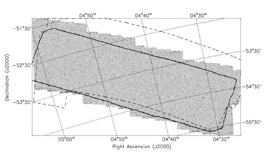
Figure 1: The 24 $\mu$m mosaic image of the SEP field. The map is shown on a linear scale ranging from $-0.09$ to 0.3 MJy sr${}^{-1}$ (roughly $-3\sigma$ to $10\sigma$). The solid contour shows the overlapping coverage in the 8.5 deg${}^{2}$ BLAST survey of this field, while the dashed contour indicates the region mapped at 90 $\mu$m by AKARI.

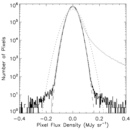
Figure 2: Distribution of pixel flux densities in the 24 $\mu$m maps. The solid light-gray histogram shows the flux distribution in the mosaic map. The black histogram shows the flux distribution in the jackknifed noise map. The dotted gray curve is the average flux distribution from simulated noise maps using the original uncertainty values determined from MOPEX, and the dashed gray curve shows this distribution after applying a correction factor of 0.68.

The total area of the SEP 24 $\mu$m map is 11.8 deg${}^{2}$, centered at (RA, Dec) $=(04^{\mathrm{h}}43^{\mathrm{m}}25.6^{\mathrm{s}}$, $-53\hbox{${}^{\circ}$}36\arcmin 41\arcsec)$. Due to the overlap of the AORs used to map the full region, the coverage in the mosaic image is non-uniform, as demonstrated in Figure 3. The median $1\sigma$ depth is 47 $\mu$Jy beam${}^{-1}$ and ranges from 31-110 $\mu$Jy beam${}^{-1}$ over the inner 10 deg${}^{2}$. Assuming a confusion limit (one source per 30 beams) of $\sim 200$ $\mu$Jy, estimated from the 24 $\mu$m number counts derived in papovich04 and sanders07, confusion effects on the map properties should be small, but non-negligible.

Figure 3: Histogram of the pixel uncertainties for the 24 $\mu$m mosaic map (scaled by a factor of 0.68), demonstrating the non-uniform coverage in this map.

The spacecraft astrometry is reported to be known to better than 1.4″. We check for a systematic shift in the astrometry by stacking the 24 $\mu$m map at the positions of 65 stars located within the field (all of which are detected at 24 $\mu$m). We find an offset of $(\delta\mathrm{RA},\delta\mathrm{Dec})=(+0.5\arcsec,+0.3\arcsec)$, which given our pixel scale of 2.45″ is consistent with zero. The stacked signal is well described by the 24 $\mu$m point response function (PRF) convolved with a Gaussian with $\sigma=1.4$″. This demonstrates that there are no systematic issues with the astrometry, and the pointing rms errors are as expected.

3.2 70 $\mu$m Map

For the 70 $\mu$m data, we start with the time-filtered BCD products (fBCDs, total of 66 098) provided by the SSC. The fBCDs are produced by subtracting the median of the surrounding Data Collection Events (DCEs) as a function of time per pixel, such that the majority of data artifacts caused by variation of the residuals in the slow response and latent artifacts from stimulator flashes are removed. We are left with a total of 63 168 (95.6%) fBCDs after excluding those with rms noise $>10$ MJy sr${}^{-1}$. As with the 24 $\mu$m data, we remove the background prior to mosaicing by subtracting the mode from each of the frames, and we use the MOPEX Mosaic pipeline to combine the frames into a single mosaic image. We interpolate the fBCDs onto a grid with $4.0\arcsec$ pixels (the native pixel scale), and we carry out multi-frame outlier detection as described above for the 24 $\mu$m data, masking samples that are $3\sigma$ outliers (default values in MOPEX for 70 $\mu$m data) to produce an initial mosaic image.

Even with the temporal high-pass filter, latent artifacts from stimulator flashes of the internal calibration source, which are correlated by column, are not fully removed; furthermore, the fBCDs provided by the SSC do not preserve calibration for extended sources. To improve the 70 $\mu$m image, we use a median column filter on the data (frayer06a), starting from the original BCDs and utilizing the Germanium Reprocessing Tools (GeRT) available from the SSC. This column filter introduces negative side-lobes near bright sources, so we redo the filtering in two steps: 1) starting with the initial mosaic made from the fBCDs we identify the brightest 10% of sources in the map using the Astronomical Point-Source Extractor (APEX) software; 2) we then use the GeRT to column filter the original BCDs with these sources masked. These steps further suppress latent artifacts and improve the calibration for extended sources. After refiltering the BCDs, we perform a background subtraction and use the MOPEX Mosaic pipeline to combine them into a single image as described in the previous paragraph.

The 70 $\mu$m mosaic map is shown in Figure 4. As with the 24 $\mu$m mosaic, the corresponding uncertainty image does not provide a good estimate of the $1\sigma$ uncertainty in the map; in this case it significantly underestimates the noise (see Figure 5). We use the same jackknifing technique as described in §3.1 to produce a noise realization for the 70 $\mu$m data, and we determine a correction factor of $2.55$ by comparing the flux distribution of the jackknifed map to that of simulated noise maps made from the original uncertainty image. We use this scaled uncertainty map for all analyses involving the 70 $\mu$m data.

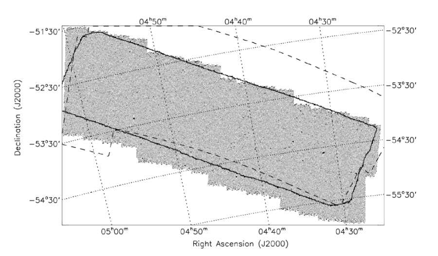
Figure 4: The 70 $\mu$m mosaic image of the SEP field. The map is shown on a linear scale ranging from $-0.9$ to 3.0 MJy sr${}^{-1}$ (roughly $-3\sigma$ to $10\sigma$). The solid contour shows the overlapping coverage in the 8.5 deg${}^{2}$ BLAST survey of this field, while the dashed contour indicates the region mapped at 90 $\mu$m by AKARI.

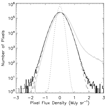
Figure 5: Distribution of pixel flux densities in the 70 $\mu$m maps. The solid light-gray histogram shows the flux distribution in the mosaic map. The black histogram shows the flux distribution in the jackknifed noise map. The dotted gray curve is the average flux distribution from simulated noise maps using the original uncertainty values determined from MOPEX, and the dashed gray curve shows this distribution after applying a correction factor of 2.55.

The total area of the 70 $\mu$m mosaic map of the SEP is 11.5 deg${}^{2}$, centered at (RA, Dec) $=(04^{\mathrm{h}}43^{\mathrm{m}}34.6^{\mathrm{s}}$, $-53\hbox{${}^{\circ}$}48\arcmin 42\arcsec)$. The noise distribution is shown in Figure 6. The median $1\sigma$ depth is 4.3 mJy beam${}^{-1}$, ranging from 2.2 to 40 mJy beam${}^{-1}$ over the inner 10 deg${}^{2}$. Given the confusion limit of $\sim 8$ mJy (frayer06a; frayer06b; frayer09), the effects of confusion on the map properties may be non-negligible.

The spacecraft astrometry for the 70 $\mu$m array is known to better than 1.7″. Since we have already verified the astrometry in the 24 $\mu$m map, we check for systematics in the 70 $\mu$m map by cross-correlating the 24 and 70 $\mu$m images. We find (as expected) a strong correlation between the two images with an astrometric offset of zero, confirming that the astrometry in the 70 $\mu$m map is good to within the 4″ pixel scale.

Figure 6: Histogram of the pixel uncertainties for the 70 $\mu$m mosaic map (scaled by a factor of 2.55).

4 Source Catalogs

4.1 24 $\mu$m Source Extraction

We use the Astronomical Point-Source Extractor (APEX) software within the MOPEX package to detect and extract sources from the 24 $\mu$m mosaic and to compute aperture photometry for these sources. We use the point-source probability (PSP) image for source detection and image segmentation. The PSP image is calculated from the background-subtracted mosaic image and the uncertainty image, filtered with the point response function (PRF, Section LABEL:ssec:prf), and represents the probability at each pixel of having a point source above the noise. Pixels that are $\geq 5\sigma$ from the mean are identified and grouped into contiguous pixel clusters; any cluster with $>20$ pixels is run through an iterative process to determine whether to split the pixel cluster into multiple sources. The PRF is then fit to the background-subtracted mosaic image at the source centroids to estimate source fluxes and refine their positions. We allow passive deblending for sources that were split into multiple pixel clusters during image segmentation, where the PRF is simultaneously fit to the blended sources. APEX computes two types of uncertainties on the PRF-fitted fluxes. The first represents the naive uncertainty from the fit, which likely underestimates the true flux uncertainty due to correlated errors. The second is computed as the quadrature sum of the data uncertainties within a box the size of the core of the PRF (extending out to $\sim 10$% of the peak). This latter quantity is used to estimate the signal-to-noise ratio (SNR) for the source candidates and generally provides a better estimate of the uncertainty.

We select an initial list of source candidates with SNR $\geq 5$. For each candidate we consider the PRF fitting to be successful if the $\chi^{2}$ per degree of freedom (reduced $\chi^{2}$) is $\chi^{2}_{\mathrm{r}}\leq 3$; this is true for 97% of the sources. The vast majority of the remaining candidates represent: 1) very bright point sources, many of them known stars in the field; 2) false detections surrounding these bright sources caused by features in the PRF (e.g., the Airy ring); 3) potential bright latent artifacts in the in-scan direction above and below a bright source; 4) extended sources; and 5) false detections arising from extended sources being split into multiple pixel clusters during image segmentation. Since this is a very large field that includes a wide range of sources, it is not possible to select a single group of settings to use for image segmentation that will be optimal in all cases. For this reason we consider the cases above by visually inspecting the mosaic image at the locations of source candidates with $\chi^{2}_{\mathrm{r}}>3$, and removing sources that are clearly false detections from the catalog.

Due to the settings used for image segmentation, false detections surrounding bright point sources arise outside of the first Airy ring ($>20$″ from the peak emission). From visually inspecting the full mosaic map we identify 90 bright point sources possibly surrounded by such false detections. Of these 65 are known stars. We identify false detections as follows: 1) using the APEX Quality Assurance (QA) pipeline, we subtract from the mosaic image a model for the PRF features at $>20$″ for each of the 90 bright sources, while retaining the center peak emission inside this radius, creating a residual image; 2) we run the same source detection and extraction algorithm as used on the mosaic image for this residual map, creating a “residual” catalog; and 3) source candidates in the original catalog that are not detected in the residual catalog are false detections and are excluded in the final 24 $\mu$m catalog. An example of how we identify false positives surrounding bright point sources is given in the upper left panel of Figure 7, which shows a 24 $\mu$m postage stamp image centered on the star SAO 233646. The small circles (diameter = 6″) and boxes mark the positions of all “sources” initially identified using APEX, where the latter represent those identified as false positives.

We additionally flag sources that remain in the residual catalog, but may also be false detections given their proximity to a bright source. Examples of these sources — which we do not remove from the final catalog — are represented by double circles in the upper left panel of Figure 7. These sources fall into three categories: 1) sources that may represent bright latent artifacts located in the in-scan direction (vertical axis in Figure 7); 2) sources that may actually be part of the PRF from the nearby bright source (e.g., radially extended artifacts in the PRF from the telescope secondary mirror support, oriented $\sim 60$${}^{\circ}$ from the scan direction); and 3) sources located within a 35″ radius of the bright source (black dashed circle in Figure 7, enclosing the second Airy ring). Some of these sources may also be false detections, and most will be poorly fit due to their proximity to a bright source. We describe the identification of false detections around extended sources in §LABEL:ssec:ext.

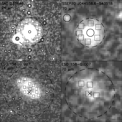
Figure 7: Examples of false positives surrounding bright point sources and extended sources in the 24 $\mu$m and 70 $\mu$m maps. All images are $2.5\arcmin\times 2.5\arcmin$ and are shown on a linear scale ranging from $-0.03$ to $0.3$ MJy sr${}^{-1}$ and $-0.3$ to 3.0 MJy sr${}^{-1}$ for the 24 $\mu$m and 70 $\mu$m data, respectively. See the text for a full description of this figure.

The final 24 $\mu$m point-source catalog is available in the electronic version of the Astrophysical Journal Supplement Series, and the first 15 entries are shown in Table 1. There is a total of 93 098 point sources with SNR $\geq 5$, after excluding known false detections. Extended sources are discussed in §LABEL:ssec:ext and listed separately in Table LABEL:tab:ecat. The number of sources identified in this field is consistent with that found in other surveys; accounting for the expected number of false positives from noise peaks (§LABEL:ssec:fdr) and incompleteness (§LABEL:ssec:comp), the number density of sources with 24 $\mu$m flux density $S_{24}>300$ $\mu$Jy is 0.8 arcmin${}^{-2}$, compared to 0.6-0.9 arcmin${}^{-2}$ observed in other deep Spitzer surveys (papovich04; sanders07).

Table 1: SEP 24 $\mu$m Point-Source Catalog

Source Name	RA	Dec	$S_{\mathrm{PRF}}\pm\sigma_{\mathrm{PRF}}$	SNR	$\chi^{2}_{\mathrm{r}}$	$S_{4.9}\pm\sigma_{4.9}$	$S_{7.4}\pm\sigma_{7.4}$	$S_{15}\pm\sigma_{15}$	Comment
	(h m s J2000)	(${}^{\circ}$ ′ ″ J2000)	($\mu$Jy)			($\mu$Jy, uncorrected)	($\mu$Jy, uncorrected)	($\mu$Jy, uncorrected)
SSEP24 J042739.3$-$551438	04 27 39.39	$-$55 14 38.0	$325\pm 25$	11	2.2	$158\pm 14$	$244\pm 22$	$284\pm 45$
SSEP24 J042835.5$-$540316	04 28 35.51	$-$54 03 16.6	$454\pm 22$	16	1.0	$255\pm 13$	$357\pm 20$	$421\pm 41$
SSEP24 J042939.9$-$554129	04 29 39.91	$-$55 41 29.4	$295\pm 36$	6.6	1.0	$160\pm 20$	$227\pm 32$	$658\pm 66$	D
SSEP24 J042940.7$-$554133	04 29 40.80	$-$55 41 33.1	$272\pm 37$	6.0	1.0	$155\pm 21$	$275\pm 32$	$747\pm 67$	D
SSEP24 J042941.6$-$554127	04 29 41.66	$-$55 41 27.9	$459\pm 36$	10	1.0	$240\pm 20$	$280\pm 32$	$411\pm 66$	D
SSEP24 J043143.5$-$550749	04 31 43.57	$-$55 07 49.4	$258\pm 20$	10	0.86	$138\pm 12$	$194\pm 18$	$391\pm 36$
SSEP24 J043410.3$-$552132	04 34 10.35	$-$55 21 32.9	$225\pm 25$	7.3	1.4	$110\pm 14$	$98\pm 22$	$14\pm 46$	P
SSEP24 J043413.3$-$552113	04 34 13.37	$-$55 21 13.3	$4358\pm 26$	140	8.8	$2252\pm 14$	$2948\pm 22$	$4323\pm 46$	S
SSEP24 J043657.3$-$545736	04 36 57.34	$-$54 57 36.1	$597\pm 21$	23	1.5	$320\pm 12$	$429\pm 18$	$659\pm 38$
SSEP24 J044008.5$-$545205	04 40 08.60	$-$54 52 05.5	$2348\pm 27$	72	1.8	$1230\pm 15$	$1518\pm 23$	$2120\pm 48$	S, D
SSEP24 J044009.5$-$545157	04 40 09.56	$-$54 51 57.2	$324\pm 27$	9.8	1.8	$214\pm 15$	$345\pm 24$	$1843\pm 49$	D, P
SSEP24 J044336.2$-$533418	04 43 36.26	$-$53 34 18.5	$143\pm 23$	5.2	0.79	$51\pm 13$	$63\pm 20$	—
SSEP24 J044541.2$-$533005	04 45 41.23	$-$53 30 05.4	$175\pm 25$	5.8	0.75	$79\pm 14$	$103\pm 21$	$195\pm 44$
SSEP24 J044938.7$-$531959	04 49 38.75	$-$53 19 59.8	$281\pm 26$	9.0	0.62	$126\pm 14$	$140\pm 22$	$199\pm 46$
SSEP24 J045209.8$-$531448	04 52 09.86	$-$53 14 48.6	$157\pm 25$	5.2	1.2	$75\pm 14$	$92\pm 22$	—

Note. — Table 1 is published in its entirety in the electronic edition of the Astrophysical Journal Supplement Series. A random sample of 15 entries are shown here for guidance regarding its form and content. The first column gives the source name using the International Astronomical Union (IAU) format. The second and third columns list the RA and Dec for each source. The fourth column gives the PRF-fitted flux density and its formal uncertainty. The fifth column gives the SNR estimate, and the sixth column gives the reduced $\chi^{2}$ for the fit. Columns 7, 8, and 9 list the (uncorrected) aperture fluxes and uncertainties (§LABEL:ssec:apphot) using 4.9″, 7.4″, and 15″ radius apertures, respectively. The last column includes comments on the sources as follows: 1) “S” - source is a known star; 2) “D” - source was passively deblended, i.e. simultaneously fit along with neighboring sources (listed consecutively in the table, having the same $\chi^{2}_{\mathrm{r}}$); and 3) “P” - source may actually be part of the PRF feature of a nearby bright source, a bright latent artifact, or be poorly fit due to its proximity to a bright source, as described in §4.1.