Spin dynamics at the singlet-triplet crossings in double quantum dot

Abstract

We simulate the control of the spin states in a two-electron double quantum dot when an external detuning potential is used for passing the system through an anticrossing. The hyperfine coupling of the electron spins with the surrounding nuclei causes the anticrossing of the spin states but also the decoherence of the spin states. We calculate numerically the singlet-triplet decoherence for different detuning values and find a good agreement with experimental measurement results of a similar setup. We predict an interference effect due to the coupling of $T_{0}$ and $T_{+}$ states.

1 Introduction

The development of a working quantum computer, based on electron spins confined in quantum dots [1, 2], has been the objective of a large field of experimentalists and theorists. One of the most important steps in realizing a spin qubit is achieving rapid control of the spin states. For two-electron quantum dots, a method based on electrical control of a singlet-triplet qubit was presented by Petta et al. [3], enabling control times of a nanosecond time scale. Recently, the control of a singlet-triplet qubit based on dynamic nuclear polarization and inhomogeneous magnetic field has been demonstrated [4].

The electrical control of spin states is based on Landau-Zener transitions between singlet and triplet states. These transitions take place when external detuning voltage is swept over singlet-triplet crossings. The coupling between singlet and triplet states in GaAs is due to the hyperfine interaction between spins of the confined electrons and spins of the surrounding nuclei [5, 6]. The transition probability depends on the sweeping rate of the detuning voltage and on the strength of the hyperfine coupling according to the Landau-Zener formula [7, 8, 9, 10]. The external magnetic field splits the triplet states into three states separated by the Zeeman splitting, $T_{+}$, $T_{0}$ and $T_{-}$. For certain detuning values, $S-T_{+}$ and $S-T_{0}$ energy differences are smaller than the hyperfine coupling. Hence, transitions from the singlet to triplet states are possible and result in a nonvanishing occupation probability of the triplet states.

Petta et al.[11, 12] studied experimentally consecutive Landau-Zener transitions between $S$ and $T_{+}$ states. They initialized a two-electron double dot so that the two electrons are in a single potential well. The Pauli exclusion principle determines that the electrons are in a singlet state. After the initialization, they rapidly moved the detuning to a value $\varepsilon$, where the potential has a double-well form and the electrons can tunnel between the wells. They held the detuning fixed for some time, and then rapidly moved the detuning back to its starting value, where they measured the probability to return as a singlet. They observed an interference pattern of decaying oscillations of the singlet probability as a function of $\varepsilon$ and time. The decay of the oscillations can be explained by the fluctuations of the nuclear spins. This experiment has recently been studied theoretically in Ref. [13].

In this paper, we study the electrical control of a two-electron double quantum dot using Landau-Zener transitions, following the cycle given above. We calculate numerically the dynamics of the setup using a 4 $\times$ 4 Hamiltonian matrix, derived by Coish and Loss [14], and evaluate numerically the probabilities of the singlet and triplet states as a function of time. We observe a similar interference pattern as observed in the experiments [11]. The occupation of the $T_{0}$ state has to be taken into account for smaller detunings. The combination of $S-T_{0}$ and $S-T_{+}$ oscillations creates a secondary interference pattern, which demands higher precision in order to be observed in the measurements.

2 Model and Method

We model the two-electron system with the Hamiltonian

$$H=\sum_{i=1}^{2}\Bigg{(}\frac{\Big{(}-i\hbar\nabla_{i}-\frac{e}{c}\mathbf{A}\Big{)}^{2}}{2m^{*}}+V(\mathbf{r}_{i},\mathbf{s}_{i})\Bigg{)}+\frac{e^{2}}{\epsilon r_{12}},$$ (1)

where the effective mass $m^{*}$=$0.067m_{e}$ and permeability $\epsilon$=12.7 are material parameters for GaAs. The external potential $V$ is divided into two parts, confinement potential $V_{C}$ and potential due to the Zeeman interaction $V_{Z}$. The smooth two-minima confinement potential, shown in Fig. 1(a), is of the form

$$V_{C}(\mathbf{r})=\frac{1}{2}m^{*}\omega^{2}[x^{2}-\lambda\tanh(x/\delta)x-\varepsilon x]+\frac{1}{2}m^{*}\omega^{2}y^{2},$$ (2)

where the confinement strength is $\hbar\omega$=3.0 meV and the parameter $\delta$=10 nm causes smoothing of the potential around $x$=0. The detuning voltage is taken into account by the parameter $\varepsilon$. The $\lambda$ parameter is used to fix the coordinates of the potential minima to $x=\pm L$, $y=0$, which is obtained using

$$\lambda=L\delta/[L(1/\cosh^{2}(L/\delta))+\delta\tanh(L/\delta)].$$ (3)

We use $L$=40 nm, and the distance of the dots is $2L$=80 nm. The potential caused by the Zeeman interaction is

$$V_{Z}(\mathbf{r},\mathbf{s})=g^{*}\mu_{B}\mathbf{B}(\mathbf{r})\cdot\mathbf{s},$$ (4)

where the Landé factor of GaAs is $g^{*}$=-0.44. The magnetic field can be divided into a homogeneous external magnetic field $\mathbf{B}_{ext}$ and an inhomogeneous random hyperfine field $\mathbf{B}_{nuc}(\mathbf{r})$.

We discretize the Hamiltonian using finite difference method and determine its eigenvalues using Lanczos diagonalization [15]. We set a numerical grid on the quantum dot, 30 grid points in x-direction and 15 points in y-direction. We simulate the fluctuations of the hyperfine field, causing the decay of the singlet-triplet oscillations, by constructing a random inhomogeneous hyperfine field. We evaluate the fluctuations of the hyperfine field by assigning a random hyperfine field vector to each grid point.

In Fig. 1(b), the energy differences between the eigenenergies of the singlet and triplet states are shown as a function of detuning for $B$= 100 mT.

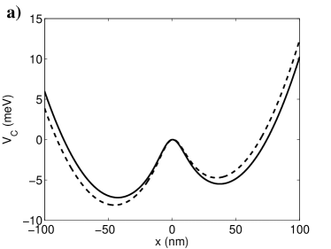
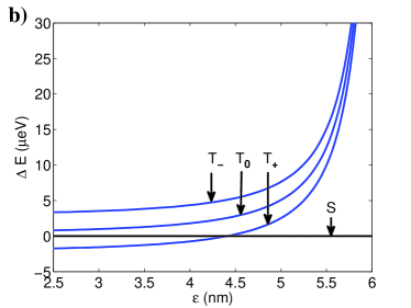
Figure 1: (Color online) (a) The confinement potential $V_{C}$ with $L$=40 nm, $\varepsilon$=5.3 nm (dashed), and $\varepsilon$=2.7 nm (solid). (b) The energy difference $\Delta E$ between the singlet state $S$ and triplet states $T_{-},T_{0}$ and $T_{+}$ as a function of the detuning $\varepsilon$. In the calculation of these energies, the hyperfine field is set to zero. The difference of $S$ and $T_{0}$ states is the exchange energy $J_{0}$. $T_{-}$ and $T_{+}$ states are separated from the $T_{0}$ state by the Zeeman splitting $\epsilon_{Z}$. The dot distance is 80 nm and magnetic field $B$=100 mT. $S$ and $T_{+}$ states cross at $\varepsilon$=4.4 nm.

The initial value of the detuning is chosen higher than 5.5 nm so that the system is initialized in the singlet state. When the detuning is lowered, the energies of the triplet states approach the energy of the singlet state. Around $\varepsilon$= 4.4 nm, $S$ and $T_{+}$ states become degenerate. For lower detunings, the energy of the $T_{0}$ state approaches asymptotically the singlet energy. For detunings lower than $\varepsilon$ = 5 nm, the singlet-triplet energy differences are so small that transitions from singlet to triplet states are possible. The coupling of the different spin states is via the hyperfine field term. For $\varepsilon<$ 3.3 nm, the $T_{0}$ state is closer in energy to $S$ state than $T_{+}$ state. Thus, the $T_{0}$ state gains larger probability than $T_{+}$ state in the transition from the $S$ state. We observe that the energy differences are not linear as a function of the detuning. A linear approximation would be valid very near to the crossing points. Hence, it is necessary to use energy values calculated here.

The energies of the excited states above the four lowest-lying states are much higher and need not to be taken into account in our analysis. We approximate the dynamics of the system using a 4 $\times$ 4 Hamiltonian, constructed in the basis of the singlet and three triplet states. For the integrals needed in the calculation of the elements of the Hamiltonian matrix, we use the shorthand notation

$$h_{i}^{\alpha}=g^{*}\mu_{B}\int\int d\mathbf{r}_{1}d\mathbf{r}_{2}\psi_{S/T}^{*}(\mathbf{r}_{1},\mathbf{r}_{2})B^{\alpha}(\mathbf{r}_{i})\psi_{S/T}(\mathbf{r}_{1},\mathbf{r}_{2}),$$ (5)

where the space parts of the wave functions $\psi_{S/T}^{*},\psi_{S/T}$ are either the singlet or triplet wave functions, depending on the calculated matrix element, $i$ is the index of the confined electron (1 or 2), and $\alpha$ is $x$, $y$, or $z$. For brevity, we introduce variables [14] that depend on $h_{1,2}$

$$h^{\alpha}=\frac{1}{2}(h_{1}^{\alpha}+h_{2}^{\alpha}),\ \delta h^{\alpha}=\frac{1}{2}(h_{1}^{\alpha}-h_{2}^{\alpha}),$$ (6)

$$h^{\pm}=h^{x}\pm ih^{y},\ \delta h^{\pm}=\delta h^{x}\pm i\delta h^{y}.$$ (7)

With these variables, the expression for the Hamiltonian matrix $H_{eff}$ in the basis {$S$, $T_{+}$, $T_{0}$, $T_{-}$} reads [14]

$$H_{eff}(\varepsilon)=\left(\begin{array}[]{cccc}0&-\delta h^{+}/\sqrt{2}&\delta h^{z}&\delta h^{-}/\sqrt{2}\\ -\delta h^{-}\sqrt{2}&J_{0}(\varepsilon)+\epsilon_{Z}+h^{z}&h^{-}/\sqrt{2}&0\\ \delta h^{z}&h^{+}/\sqrt{2}&J_{0}(\varepsilon)&h^{-}/\sqrt{2}\\ \delta h^{+}/\sqrt{2}&0&h^{+}/\sqrt{2}&J_{0}(\varepsilon)-\epsilon_{Z}-h^{z}\end{array}\right),$$ (8)

where $\epsilon_{Z}$=$g^{*}\mu_{B}B^{z}$, and $J_{0}$ is the energy difference between $S$ and $T_{0}$ states, shown in Fig. 1(b). As the detuning $\varepsilon$ depends on time, the effective Hamiltonian is also time-dependent.

In order to numerically model the experiment of Petta et al.[11] and compare the obtained singlet probabilities with the experimental data, we write the wave function of the system in the basis of the four singlet and triplet states, and the singlet and triplet probabilities are calculated from the wave function [16]. The dynamics of the wave function is calculated using the relation $\psi(t+\Delta t)=\exp(-i\Delta tH_{eff}(t)/\hbar)\psi(t)$.

In our simulation, we describe the voltage by a detuning parameter $\varepsilon$ which has length as its unit. For the initialization at $t$=0, we set detuning 3 nm above its minimum value, which guarantees that the system is initialized in the singlet state. We model the sweeping of the detuning by lowering it to a minimum value in 0.2 ns. This minimum value varies between 2.5 and 5.5 nm.

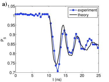
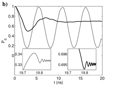
Figure 2: (Color online) (a) The singlet probability $P_{S}$, as a function of the time $t$. The blue spheres correspond to measurement results of Petta et al. (upper part of Fig. 3(d) in Ref. [11]), black curve represents our theoretical fit for detuning $\varepsilon$=4.0 nm, averaged over 1000 realizations. The theoretical data is shifted by 10 ns, because there is a delay in the experiments before singlet-triplet oscillations emerge. (b) The singlet probabilities, as a function of the time $t$. The detuning $\varepsilon$ is 4.3 nm. The gray line is singlet probability calculated for a single realization, black line is an average over 1000 realizations. The insets show the probabilities when detuning is changed back to its initial value in 0.2 ns. After passing the Landau-Zener crossing during the detuning sweeping back to its initial value at 19.8 ns, the oscillations are rapidly damped.

The parameters used in our simulation are determined by fitting the theoretical results to the experimental singlet probability shown in the upper part of Fig. 3(d) of Ref. [11]. The fitting is shown in Fig. 2(a). We set the detuning in our fit to $\varepsilon$=4.0 nm so that the oscillation periods, which depend only on the $S$-$T_{+}$ energy difference, are the same. We omit the first 10 ns of the experimental data when the singlet probability stays constant. After 10 ns, the experimental singlet probability drops to 0.7 and then oscillates with period around 4 ns. The oscillation decays towards value 0.84. We set the hyperfine field strength and the sweeping time to such values that the theoretical singlet-triplet oscillation approaches 0.84 and the oscillation decays similarly with the experimental data. Best fit is obtained with uniformly distributed hyperfine field values between -7.5 mT and 7.5 mT. The root mean square of the hyperfine field is 4.3 mT. In the experiments, the rms value has been around 2 mT [17]. The difference between these values might be due to the different strengths of the confinement potential used in the experiments and numerical model. The resulting hyperfine coupling of the singlet and triplet states $\delta h^{z}$ is tens of neV, which is in the same magnitude than the experimental value 60 neV. We average the spin dynamics over 1000 random hyperfine field realizations. As the sum of uniformly distributed random numbers is Gaussian, our simulation corresponds to a Gaussian distributed hyperfine field. We sweep the detuning to the minimum value in 0.2 ns. With these parameter values, the decaying oscillations are similar with the experimental data. Although the measured value may deviate from real singlet probability, this fit gives the relevant scale for the parameters.

The decay of the oscillations is due to the finite temperature of the nuclear spins. Figure  2(b) shows singlet oscillations calculated for a single realization and an average over 1000 realizations. We observe for the single realization a non-decaying oscillation. For different realizations, the oscillations have different periods and amplitudes. As a result, the averaged oscillations decay and approach a constant value, as the solid line in Fig. 2(b) indicates. The detuning is kept in the minimum value for 0-28 ns. The sweeping of the detuning back to the initial value in 0.2 ns does not significantly change the singlet probability. If we would model the experiment rigorously, we should calculate separately each detuning cycle for different waiting times, sweep the detuning back to the original value, and save the singlet probability at the end. However, the singlet probability does not significantly change during the return sweep. In the insets of Fig. 2(b), the singlet-triplet oscillations during the sweeping back to initial detuning are shown for a single realization and for an average over 1000 realizations. The sweeping takes place between 19.7 ns and 19.9 ns. When Landau-Zener crossing point is passed at 19.8 ns, the singlet-triplet oscillation stops and after that the faster oscillations decay very rapidly. In practice, the oscillation freezes at the value it had at the crossing point. During the 0.1 ns sweep from the minimum value of the detuning to the crossing point, the singlet probability changes less than 0.01. Hence, we may end the simulation just before the detuning sweep and approximate the final value of the singlet probability by using the value the probability has just at the beginning of the detuning sweep. This approximation enables calculation of the final singlet probabilities for each waiting time in a single run. We only have to make new runs for different detuning values. We set the magnetic field to 100 mT, as in the experiment.

The analysis of the experiment of Petta et al. could be done using a three-level model, as it turns out that the $T_{-}$ state remains unoccupied. It might even be possible to obtain an exact analytical solution for the singlet probability. A similar model was used to study a recent experiment [18], where a Josephson qubit was coupled to two two-level systems. In this case, the two-level systems are not coupled to each other, making the calculation of the time dependence easier. We have the additional difficulty of $T_{+}$-$T_{0}$ coupling, and the resulting singlet probability should be averaged over Gaussian distribution. As our numerical method is reasonably fast to calculate, an analytical approach would not be practical for our study.

3 Results and Discussion

Now after we have obtained the necessary parameters, we can vary the detuning $\varepsilon$ and also compare results with the experiment of Petta et al.[11]. The calculated singlet probabilities for detuning values between 2.5 and 5.5 nm are shown in Fig. 3 (single realization) and Fig. 4 (average over 1000 realizations). The single realization case is shown because the interference effects are then easier to observe.

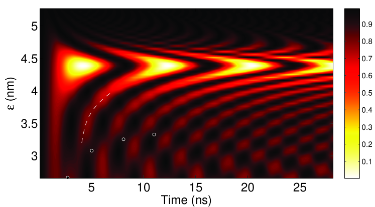
Figure 3: (Color online) Probability $P_{S}$ of the singlet state $S$ as a function of time $t$ and detuning $\varepsilon$ calculated for a single hyperfine field realization. The darker colors indicate increasing $P_{S}$. The white dashed line indicates one of the interference lines line due to the $S$-$T_{+}$ oscillation and black spheres show the point in the interference lines where the singlet probability is diminished due to the $S$-$T_{0}$ oscillation.

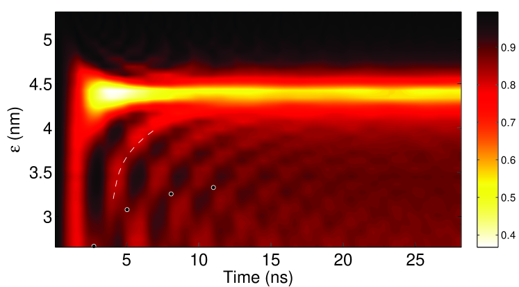
Figure 4: (Color online) Same as Fig. 3, but here the singlet probability $P_{S}$ is calculated using an average of 1000 hyperfine field realizations and the color scale is different.

We have plotted the singlet probability as a function of time (x-axis) and detuning (y-axis). The darker colors indicate increasing singlet probability. For detunings above the $S$-$T_{+}$ crossing point $\varepsilon$=4.4 nm, the singlet probability does not change considerably from value 1, making the upper part of the figure dark. The period of the singlet probability oscillations depends inversely on the energy difference between $S$ and $T$ states. In Fig. 3, we observe that the oscillation period diminishes, when detuning values are further from the Landau-Zener crossing and the $S$-$T$ energy difference increases. At the crossing, the amplitude and period of the oscillation are largest. The minima of the oscillations form observable red lines on the dark background. One of them is accentuated with a white dashed line. The same phenomena are present in Fig. 4, but the averaging makes the figure more blurred. When the detuning is near the crossing point, the singlet oscillation drops from 1 to 0.5 and the later oscillations are rapidly damped. This causes the yellow band in the middle of the figure. The oscillations for detunings above the crossing point are barely visible. For detunings under the crossing point, the oscillations are damped and the bands formed by the minima of the probability are not so clear.

The occupation probability of the $T_{0}$ state affects the singlet-triplet oscillations by damping the oscillations for certain detuning values. The red interference lines are then slightly narrower. These narrower places in the lines form a secondary interference pattern, one of those is indicated with black spheres in the figure. This pattern is better seen in Fig. 3, where the widening and narrowing of the lines is clearly observable. For example, for detuning $\varepsilon$= 2.9 nm, the interference of the triplet states at 3.5 ns causes a dip in the peak of the singlet probability in Fig. 5. This effect is quite small and not easy to observe experimentally. In the situation where the energy of the $S$ state is closer in energy to $T_{0}$ state than to $T_{+}$ state, the period is given by the $S$-$T_{0}$ energy difference. Hence, when these two energy differences are equal at $\varepsilon$=3.3 nm, the singlet-triplet oscillation period has its smallest value 3.2 ns. The interference lines are not symmetric with respect to the detuning of the singlet-triplet crossing point. This is due to the asymmetry of the exchange energy around the crossing point as a function of detuning. As the exchange energy increases rapidly for detunings above the crossing point, the period of the oscillation decreases swiftly and the interference lines disappear. The features in the figure above $\varepsilon$=4.5 nm would vanish completely if the slope of the exchange energy were steeper.

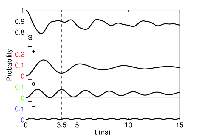
Figure 5: (Color online) The singlet and triplet probabilities, as a function of the time $t$. The detuning $\varepsilon$ is 2.9 nm. The dashed line at 3.5 ns marks the point where the occupation of $T_{0}$ state diminishes the probability of the $S$ state.

When we compare our results with experiments of Petta et al. [11], we find that the interference patterns of the oscillations are quite similar. The contrast of the interference lines is better in the experimental figure. This might be due to the small number of detuning sweeps used in the averaging of due to correlations between different sweeps. The experimental pattern has an area where the singlet probability remains 1 before the oscillation begins. The oscillations start later for higher values of detuning, probably due to the smoothed voltage pulse profile used in the experiment. We did not model this effect in our calculation. For detunings above the $S$-$T_{+}$ crossing, our data shows small oscillations that are missing from the experimental data. These are, however, much smaller than in the model of Ref. [13]. Probably the measurement accuracy is not sufficiently high for the observation of these small oscillations. At the singlet-triplet crossing ($\varepsilon\approx$ 4.4 nm), the numerical singlet probability is smaller than 0.5 at 5 ns. In the experiment this minimum is not seen, but the singlet probability goes to 0.5 without having decaying oscillations. This might be due to the smoothed pulse profile, which causes over 15 ns delay of the singlet-triplet oscillation at the $S$-$T_{+}$ crossing.

In the measurements of Petta et al. [11], the interference effects due to the occupation of $T_{0}$ state are not visible. The resolution of the experimental data is not high enough to observe the interference clearly, but if we compare the data with Fig. 3, we find that the widening and narrowing of the bands could have taken place in the experiments. With the experimental resolution, the oscillations for the lower detunings look quite similar. If the singlet probability could be measured more accurately, it would be possible to detect this interference and observe whether both $T_{0}$ and $T_{+}$ states are occupied. If it is the case that the experiments do not exhibit this interference, the reason for the disappearance of $S$-$T_{0}$ oscillations could be that the $S$-$T_{0}$ coupling is much stronger than $S$-$T_{+}$ coupling, and the oscillations decay very rapidly. Or the $S$-$T_{0}$ coupling is much weaker and the $S$-$T_{0}$ oscillation period is longer than the measurement time.

A small nuclear polarization ($\sim$0.5%) could prolong the singlet-triplet dephasing time by two orders of magnitude, as predicted by Ramon and Hu [19]. Then, the polarization would not change the $S$-$T_{+}$ crossing point but could weaken the $S$-$T_{0}$ coupling so that the $T_{0}$ state does not become occupied during the measurement, even for detunings in the vicinity of $S$-$T_{0}$ crossing. In that case, the interference effects due to $T_{0}$ state would vanish and the smallest possible period of singlet-triplet oscillations would be given by $S$-$T_{+}$ oscillations at the Zeeman energy, resulting in a minimum period 1.6 ns observed by Petta et al. [11].

The results we obtained do not considerably depend on the exact form of the potential. We used the potential given by Eq. (2), but any other smooth double-well potential would produce similar results for the singlet-triplet oscillations. The time dependence of the detuning was taken to be linear here. Other monotonic time dependencies would not have great effect on the singlet probabilities, because the transitions from singlet to triplet states occur at the crossing points, where the time dependence can be approximated by a linear fit. The form of the time dependence does not matter outside the crossing points.

In summary, we have studied singlet-triplet decoherence in a two-electron double quantum dot with an external detuning voltage. We calculated the singlet probability as a function of time for different detunings. The interference pattern of the singlet probability is very similar with the recent experimental results and the decay of the oscillations is described somewhat better than in another theoretical study of the same experiment [13]. Our results indicate that also $T_{0}$ state could be occupied, even if $S$-$T_{0}$ crossing point is not within the range of detuning values used. When the system is in the proximity of the crossing point, transition to $T_{0}$ state is possible. In addition, we predict an observable effect in the interference pattern due to the occupation of $T_{0}$ state. If the measurement process affects the $S$-$T_{0}$ coupling but not the $S$-$T_{+}$ coupling, the interference effects could disappear, which we suggest might be the case in the measurement of Petta et al.[11].

References

References

- [1] Loss D and DiVincenzo D P 1998 Phys. Rev. A 57 120
- [2] Hanson R, Kouwenhoven L P, Petta J R, Tarucha S and Vandersypen L M K 2007 Rev. Mod. Phys. 79 1217
- [3] Petta J R, Johnson A C, Taylor J M, Laird E A, Yacoby A, Lukin M D, Marcus C M, Hanson M P and Gossard A C 2005 Science 309 2180
- [4] Foletti S, Bluhm H, Mahalu D, Umansky V and Yacoby A 2009 Nature Phys. 5 903
- [5] Khaetskii A V, Loss D and Glazman L 2002 Phys. Rev. Lett. 88 186802
- [6] Merkulov I A, Efros A L and Rosen M 2002 Phys. Rev. B 65 205309
- [7] Landau L 1932 Phys. Z. Sowjetunion 2 46
- [8] Zener C 1932 Proc. R. Soc. A 137 696
- [9] Wittig C 2005 J. Phys. Chem. B 109 8428
- [10] Shevchenko S N, Ashhab S and Nori F 2010 Phys. Rep. 492 1
- [11] Petta J R, Lu M and Gossard A C 2010 Science 327 669
- [12] Burkard G 2010 Science 327 650
- [13] Ribeiro H, Petta J R and Burkard G 2010 Phys. Rev. B 82 115445
- [14] Coish W A and Loss D 2005 Phys. Rev. B 72 125337
- [15] Särkkä J and Harju A 2008 Phys. Rev. B 77 245315
- [16] Särkkä J and Harju A 2009 Phys. Rev. B 80 045323
- [17] Taylor J M, Petta J R, Johnson A C, Yacoby A, Marcus C M and Lukin M D 2007 Phys. Rev. B 76 035315
- [18] Sun G, Wen X, Mao B, Chen J, Yu Y, Wu P and Han S 2010 Nature Commun. 1 51
- [19] Ramon G and Hu X 2007 Phys. Rev. B 75 161301