Interference Channel with an Out-of-Band Relay

Abstract

A Gaussian interference channel (IC) with a relay is considered. The relay is assumed to operate over an orthogonal band with respect to the underlying IC, and the overall system is referred to as IC with an out-of-band relay (IC-OBR). The system can be seen as operating over two parallel interference-limited channels: The first is a standard Gaussian IC and the second is a Gaussian relay channel characterized by two sources and destinations communicating through the relay without direct links. We refer to the second parallel channel as OBR Channel (OBRC).

The main aim of this work is to identify conditions under which optimal operation, in terms of the capacity region of the IC-OBR, entails either signal relaying and/or interference forwarding by the relay, with either a separable or non-separable use of the two parallel channels, IC and OBRC. Here “separable” refers to transmission of independent information over the two constituent channels.

For a basic model in which the OBRC consists of four orthogonal channels from sources to relay and from relay to destinations (IC-OBR Type-I), a condition is identified under which signal relaying and separable operation is optimal. This condition entails the presence of a relay-to-destinations capacity bottleneck on the OBRC and holds irrespective of the IC. When this condition is not satisfied, various scenarios, which depend on the IC channel gains, are identified in which interference forwarding and non-separable operation are necessary to achieve optimal performance. In these scenarios, the system exploits the “excess capacity” on the OBRC via interference forwarding to drive the IC-OBR system in specific interference regimes (strong or mixed).

The analysis is then turned to a more complex IC-OBR, in which the OBRC consists of only two orthogonal channels, one from sources to relay and one from relay to destinations (IC-OBR Type-II). For this channel, some capacity resuls are derived that parallel the conclusions for IC-OBR Type-I and point to the additional analytical challenges.

I Introduction

Modern wireless communication networks are characterized by the coexistence of an increasing number of interfering devices and systems. While this often leads to an overall system performance that is limited by mutual interference, the presence of many independent wireless devices may also potentially offer new opportunities and performance benefits by allowing cooperation. Opportunities for cooperation are further enhanced for multistandard terminals that are able to communicate simultaneously over multiple radio interfaces, and thus to interact and cooperate with devices belonging to different systems and networks. For instance, many current wireless terminals are equipped with a 3G cellular transceiver along with a Wi-Fi interface. This paper focuses on investigating the advantages of cooperation in interference-limited scenarios where cooperation is enabled by orthogonal radio interfaces and multistandard terminals.

To fix the ideas on the problem of interest, consider Fig. 1, where a two-user Interference Channel (IC) operating over a certain bandwidth and using a certain radio communication standard (say, Wi-Fi) is aided by a relay that operates over an orthogonal bandwidth and uses a possibly different standard (say, Bluetooth). For this reason, we refer to the relay as an Out-of-Band Relay (OBR). Sources and destinations are assumed to be multistandard, thus being able to transmit and receive, respectively, over both radio interfaces. The system can be seen as being characterized by two parallel channels, in which the first (i.e., the Wi-Fi channel) is a standard Gaussian IC, and the second (i.e., the Bluetooth channel) is a particular Gaussian relay channel. Specifically, the second channel is characterized by two sources and destinations communicating through the relay without the direct links between sources and destinations [37]-[39]. We refer to it as OBR Channel (OBRC). The absence of a direct link on the OBRC can be justified in case the wireless radio interface used on the OBRC has a shorter range than the one used over the IC, as it is the case for the Wi-Fi/ Blueetooth example. We are interested in the optimal operation on the overall system, IC and OBRC, which is termed IC with an OBR or IC-OBR.

As explained above, the two components of an IC-OBR model are an IC (see, e.g, [32] for a summary of the state of the art on the subject) and the OBRC. Assuming a half-duplex relay, the latter is modelled in two different ways (see Fig.1): (i) IC-OBR Type-I: The OBRC is operated by assuming orthogonal transmissions (e.g., via TDMA or FDMA) over the four Gaussian links connecting sources to relay and relay to destinations; (ii) IC-OBR Type-II: The OBRC is more generally operated by orthogonalizing the Gaussian multiple access channel between the two sources and the relay and the broadcast channel from relay to destinations. It is noted that relay models similar to the assumed OBRC have been recently studied in [37] from an outage perspective and in [38][39] assuming (symmetric) two-way communications (see also [28][29]). Overall, it is remarked that general capacity results are unavailable for both component channels of a IC-OBR, namely the IC and OBRC.

Beside the connection with the literature on the two individual component channels, briefly reviewed above, the considered model is related to, and inspired by, two recent lines of work. The first deals with relaying in interference-limited systems, where, unlike the IC-OBR, the relay is assumed to operate in the same band as the IC [16]-[22]. These works reveal the fact that relaying in interference-limited systems offers performance benefits not only due to signal relaying, as for standard relay channels (see, e.g., [4]), but also thanks to the novel idea of interference forwarding. According to the latter, the relay helps by either reinforcing the interference received at the undesired destination so as to facilitate interference stripping, or by conversely reducing the interference via negative beamforming. Achievable schemes incorporating these operations for a Gaussian system are developed in [14] [16] [22], while [18] deals with a discrete-memoryless model and [40] derives an upper bound on the capacity region by allocating infinite power to the relay (see also [24] for a review).

A second related line of work deals with communications over parallel ICs (albeit the considered OBRC is not a conventional IC). As shown in [41] [42] [44], optimal operation over parallel ICs, unlike scenarios with a single source or destination, typically entails joint coding over the parallel channels. In other words, the signals sent over the parallel ICs need to be generally correlated to achieve optimality, and thus a separable approach, whereby the parallel channels are treated independently, is in general not sufficient. To elaborate, recall that the most general transmission scheme for a regular IC involves splitting of each source’s message into both private and common submessages, where the first is treated as noise at the unintended destination, while the latter is jointly decoded with the messages of the intended source. Now, in the presence of parallel ICs, given the above, the question arises as to what type of information, either private or common, should be sent over the parallel channels. For instance, the original work [41] derives conditions under which correlated transmission of private messages is optimal and [42] considers the optimality of common information transmission, whereas in [44] scenarios are found for which sending both correlated private and common messages is optimal. We refer to [42], [43] and [44] for a summary of special cases in which a separable approach is instead optimal.

For the IC-OBR under study, the main issue we are interested in is assessing under which conditions the OBRC should be optimally used for either or both signal relaying or interference forwarding, and by following a separable or non-separable transmission strategy over the parallel channels given by the IC and the OBRC. The main contribution of the paper is the identification of a number of such scenarios, which we classify as being characterized by relay-to-destinations bottleneck or excess rate conditions, for both IC-OBR Type-I and Type-II and assuming both fixed and variable bandwidth allocations on the OBRC.

The paper is organized as follows. In Section II, we give the system models of IC-OBR Type-I and Type-II channels. Section III gives a general outer bound and achievable region for IC-OBR Type-I for both fixed and variable OBRC bandwidth allocations. Capacity results are established for both cases. In Section IV, we give outer bounds on the capacity region for IC-OBR Type-II. Conditions for the optimality of signal relaying and/or interference forwarding for IC-OBR Type-II are established in this section. Finally, we conclude the paper in Section V.

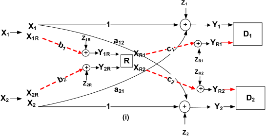
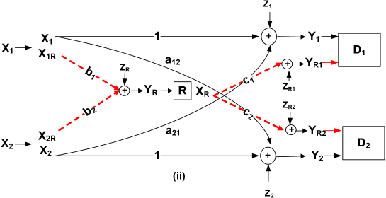
Figure 1: Interference Channel (IC) with an out-of-band relay (OBR). The OBR channel (OBRC) has $\eta$ channel uses for each channel use of IC. (i) IC-OBR Type-I: The OBRC is divided into four Gaussian orthogonal channels with $\eta_{iR}$, $\eta_{Ri}$, $i=1,2$, channel uses each; (ii) IC-OBR Type II: The OBRC is divided into two orthogonal channels with $\eta_{MAC}$, $\eta_{BC}$ channel uses.

Notation: We define $\mathcal{C}(x)=1/2\log_{2}(1+x)$.

II System Models

We investigate the IC-OBR models shown in Fig. 1, which we refer to as IC-OBR Type-I and Type-II. In both models, the sources $S_{1}$ and $S_{2}$ communicate to their respective destinations $D_{1}$ and $D_{2}$ via two orthogonal channels, namely a Gaussian IC and the out-of-band relay channel (OBRC), where the latter is characterized by $\eta\geq 0$ channel uses per channel use of the IC. In pratice, parameter $\eta$ can be thought of as the ratio between the bandwidth of the OBRC and of the IC. Specifically, each source $S_{i},$ $i=1,2,$ wishes to send a message index $W_{i},$ uniformly drawn from the message set $[1,2^{nR_{i}}]$ , to its destination $D_{i},$ with the help of an OBR, which operates half-duplex. Notice that $n$ is the number of channel uses of the IC available for communication of the given messages (which yields $\eta n$ channel uses for the OBRC), so that $R_{i}$ is the rate of the $i$th pair ($S_{i},D_{i}$) in terms of bits per IC channel use.

The signals received on the IC by the two receivers $D_{1}$ and $D_{2}$ in channel use $t=1,...,n$ are given as, respectively,

$$Y_{1,t} =X_{1,t}+a_{21}X_{2,t}+Z_{1,t}$$ (1a)

$$Y_{2,t} =a_{12}X_{1,t}+X_{2,t}+Z_{2,t},$$ (1b)

where $$X_{i,t}\in\mathbb{R} S_{i} \frac{1}{n}\sum_{t=1}^{n}E[X_{i,t}^{2}]\leq P_{i} Z_{i,t}$$ represents the (real) input symbol of source , which satisfies the power constraint , and are independent identically distributed (i.i.d.) zero-mean Gaussian noise processes with unit power. The two IC-OBR models studied in the following differ in the way the OBRC is operated, as discussed below. Both models assume a half-duplex relay.

II-A IC-OBR Type-I

In the IC-OBR Type-I model, shown in Fig.1-(i), the OBRC bandwidth (or equivalently the set of channel uses $\eta n$) is partitioned into four orthogonal Gaussian channels, corresponding to different source-to-relay and relay-to-destination pairs. This can be realized by orthogonal access schemes such as TDMA or FDMA. Specifically, we have two Gaussian channels from sources $S_{i}$ to relay $R$ with fraction of channel uses $\eta_{iR}$, $i=1,2,$ and two Gaussian channels from the relay $R$ to destinations $D_{i},$ $i=1,2,$ with fraction of channel uses $\eta_{Ri}.$ We have $\sum_{i=1}^{2}(\eta_{iR}+\eta_{Ri})=\eta$. The signals received by the relay $R$ over the OBRC on the source-to-relay channels are given by

$$Y_{iR,t}=b_{i}X_{iR,t}+Z_{iR,t},$$ (2)

for $t=1,...,\eta_{iR}n$ and $i=1,2,$ whereas the signals received at the destination over the OBRC on the relay-to-destination channels are given by

$$Y_{Ri,t}=c_{i}X_{Ri,t}+Z_{Ri,t},$$ (3)

for $t=1,...,\eta_{Ri}n$, $i=1,2,$ where ($Z_{iR,t},Z_{Ri,t})$ are i.i.d. zero-mean Gaussian noise processes with unit power. We assume power constraints $\frac{1}{n}\sum_{t=1}^{\eta_{iR}n}E[X_{iR,t}^{2}]\leq P_{iR}$, and $\frac{1}{n}\sum_{t=1}^{\eta_{Ri}n}E[X_{Ri,t}^{2}]\leq P_{Ri}$, $i=1,2$. The rationale behind this power constraint assumption arises for the scenarios such as the relay transmits using TDMA with per-symbol power constraints, or employs FDMA transmission with spectral mask constraints. Another model that encompasses this assumption is where the relay communicates with the destinations using two distinct radio interfaces with different transceivers.

A $(2^{nR_{1}},2^{nR_{2}},n)$ code for the IC-OBR type-I is defined by: (a) The encoding functions at the sources $S_{i},$ $i=1,2,$ given by

$$f_{i}^{(n)}\text{: }[1,2^{nR_{i}}]\rightarrow\mathbb{R}^{n}\times\mathbb{R}^{\eta_{iR}n}$$ (4)

which maps a message $W_{i}\in[1,2^{nR_{i}}]$ into the codewords ($X_{i}^{n},X_{iR}^{\eta_{iR}n})=f_{i}^{(n)}(W_{i})$ to be transmitted on the IC and OBRC, respectively; (b) The encoding function $g^{(n)}$ at the relay given by

$$g^{(n)}\text{: }\mathbb{R}^{\eta_{1R}n}\times\mathbb{R}^{\eta_{2R}n}\rightarrow\mathbb{R}^{\eta_{R1}n}\times\mathbb{R}^{\eta_{R2}n},$$ (5)

which maps the received signal to the codewords ($X_{R1}^{n\eta_{R1}},X_{R2}^{n\eta_{R2}})=g^{(n)}(Y_{R1}^{\eta_{1R}n},Y_{R2}^{\eta_{2R}n})$, $i=1,2,$ that are sent to the destinations; (c) The decoding functions at the destinations $D_{i}$, denoted by $h_{i}^{(n)}$, $i=1,2,$ with,

$$h_{i}^{(n)}\text{: }\mathbb{R}^{n}\times\mathbb{R}^{\eta_{Ri}n}\rightarrow[1,2^{nR_{i}}]$$ (6)

which maps the received signal via the IC, $Y_{i}^{n}$ and OBRC $Y_{Ri}^{\eta_{Ri}n}$ into the estimated message $\widehat{W}_{i}=h_{i}^{(n)}(Y_{i}^{n},Y_{Ri}^{\eta_{Ri}n})$.

II-B IC-OBR Type-II

The IC-OBR Type-II model, shown in Fig.1-(ii), the OBRC is orthogonalized into two channels, one being a multiple-access channel (MAC) from $S_{1}$ and $S_{2}$ to $R,$ with fraction of channel uses $\eta_{MAC},$ and the other being a broadcast channel (BC) from $R$ to $D_{1}$ and $D_{2}$, with fraction of channel uses $\eta_{BC}$. We have $\eta_{MAC}+\eta_{BC}=\eta$. The received signal at the relay $R$ over the OBRC is given by

$$Y_{R,t}=b_{1}X_{1R,t}+b_{2}X_{2R,t}+Z_{R,t}$$ (7)

for $t=1,...,\eta_{MAC}n$; and the signal received at destination $D_{i}$ over the OBRC is

$$Y_{Ri,t}=c_{i}X_{R,t}+Z_{Ri,t},\mbox{ }i=1,2,$$

for $t=1,...,\eta_{BC}n$, $i=1,2.$ We have the power constraints $\frac{1}{n}\sum_{t=1}^{\eta_{MAC}n}E[X_{iR,t}^{2}]\leq P_{iR}$, and $\frac{1}{n}\sum_{t=1}^{\eta_{BC}n}E[X_{R,t}^{2}]\leq P_{R}$.

A $(2^{nR_{1}},2^{nR_{2}},n)$ code for the IC-OBR Type-II is defined similar to codes for IC-OBR Type-I with the difference that the encoding function $g^{(n)}$ at the relay is modified as

$$g^{(n)}\text{: }\mathbb{R}^{\eta_{MAC}n}\rightarrow\mathbb{R}^{\eta_{BC}n},$$

which maps the received signal $Y_{R}^{\eta_{MAC}n}$ into the transmitted codeword $X_{R,t}^{\eta_{BC}n}=g^{(n)}(Y_{R}^{\eta_{MAC}n}).$

Note that IC-OBR Type-I is a special case of Type-II, obtained by orthogonalizing the MAC and the BC.

II-C Achievable Rates for Fixed and Variable OBRC Bandwidth Allocation

Following conventional definitions, we define the probability of error as the probability that any of the two transmitted messages is not correctly decoded at the intended destination. Achievable rates ($R_{1},R_{2}$) are then defined for two different scenarios: (a) Fixed OBRC bandwidth allocation: Here, the bandwidth allocation parameters over the OBRC, namely ($\eta_{R1},\eta_{R2},\eta_{1R},\eta_{2R}$) for IC-OBR Type-I and ($\eta_{MAC},\eta_{BC}$) for Type-II, are considered to be given and fixed. Therefore, a rate pair ($R_{1},R_{2}$) is achievable if a coding scheme can be found that drives the probability of error to zero for the given (feasible) bandwidth allocation parameters; (b) Variable OBRC bandwidth allocation: Here the bandwidth allocation can be optimized, so that a rate pair ($R_{1},R_{2}$) is said to be achievable if a coding scheme exists that drives the probability of error to zero for some feasible bandwidth allocation parameters. The capacity region is in both cases the closure of the set of all achievable rates.

III Analysis of IC-OBR Type-I

In this section, we investigate the IC-OBR Type-I system described in Sec. II. We consider outer bounds and inner bounds to the achievable rate regions for both fixed and variable OBRC bandwidth allocation. It is noted that the results for fixed OBRC were partly presented in [24].

III-A Outer Bound

In this section, we first present a general outer bound to the capacity region of an IC-OBR in terms of multi-letter mutual informations (Proposition 1). This bound is then specialized to a number of special cases of interest, allowing the identification of the capacity region of IC-OBR for various scenarios.

Proposition 1 (Outer bound for IC-OBR Type-I): For fixed OBRC bandwidth allocation, the capacity region of the IC-OBR Type-I is contained within the set of rates $(R_{1},R_{2})$ satisfying

$$\lim_{n\rightarrow\infty}\mbox{closure}\bigg{(}\bigcup_{p(x_{1}^{n},x_{2}^{n})=p(x_{1}^{n})p(x_{2}^{n})}\big{\{}(R_{1},R_{2})\text{:}$$

$$R_{1}\leq\frac{1}{n}I(X_{1}^{n};Y_{1}^{n})+\min\left\{\eta_{1R}\mathcal{C}(b_{1}^{2}P_{1R})+\eta_{2R}\mathcal{C}(b_{2}^{2}P_{2R}),\eta_{R1}\mathcal{C}(c_{1}^{2}P_{R1})\right\}$$

$$R_{1}\leq\frac{1}{n}I(X_{1}^{n};Y_{1}^{n}|X_{2}^{n})+\min\left\{\eta_{1R}\mathcal{C}(b_{1}^{2}P_{1R}),\eta_{R1}\mathcal{C}(c_{1}^{2}P_{R1})\right\}$$

$$R_{2}\leq\frac{1}{n}I(X_{2}^{n};Y_{2}^{n})+\min\left\{\eta_{1R}\mathcal{C}(b_{1}^{2}P_{1R})+\eta_{2R}\mathcal{C}(b_{2}^{2}P_{2R}),\eta_{R2}\mathcal{C}(c_{2}^{2}P_{R2})\right\}$$

$$R_{2}\leq\frac{1}{n}I(X_{2}^{n};Y_{2}^{n}|X_{1}^{n})+\min\left\{\eta_{2R}\mathcal{C}(b_{2}^{2}P_{2R}),\eta_{R2}\mathcal{C}(c_{2}^{2}P_{R2})\right\}\big{\}}\bigg{)}$$ (8)

where the union is taken with respect to all multi-letter input distributions $p(x_{1}^{n})p(x_{2}^{n})$ that satisfy the power constraints $1/n\sum_{t=1}^{n}\mbox{E}[X_{i,t}^{2}]\leq P_{i}$, $i=1,2$. With variable OBRC bandwidth allocation, an outer bound is given as above but with the union in (8) taken also with respect to all parameters $\eta_{iR},\eta_{Ri}$, $i=1,2,$ such that $\sum_{i=1}^{2}(\eta_{iR}+\eta_{Ri})=\eta$.

Proof: Appendix A.

III-B Achievable Rate Region

In this section, we derive an achievable rate region for the IC-OBR Type-I. We propose to use a rate splitting scheme similar to the standard approach for ICs [3] [6]. Specifically, we split the message of each user into private and common messages, where the private message of each source is to be decoded only by the intended destination and the common is to be decoded at both intended and interfered destinations. However, private and common parts are further split into two (independent) messages as follows. One of the private message splits is sent over the IC and the other one over the OBRC. As for the common message, both parts are sent over the IC, but one of the two is also sent over the OBRC to the interfered destination for interference cancellation. More specifically, we have the following four-way split of each message $W_{i},$ $W_{i}=(W_{iR},W_{ip},W_{ic^{\prime}},W_{ic^{\prime\prime}})$, $i=1,2$, where: (i) $W_{iR}\in[1,...2^{nR_{iR}}]$ is a private message that is transmitted via the OBRC only, directly to $D_{i}$. Notice that since the OBR has orthogonal channels to the IC, this message is conveyed interference-free to $D_{i}$; (ii) $W_{ip}\in[1,...2^{nR_{ip}}]$ is a private message that is transmitted over the IC, decoded at $D_{i}$ and treated as noise at $D_{j},$ $j\neq i$; (iii) $W_{ic^{\prime}}\in[1,2^{nR_{ic^{\prime}}}]$ is a common message that is transmitted over the IC and OBRC. Specifically, the relay conveys $W_{ic^{\prime}}$ to $D_{j}$ only, $j\neq i,$ to enable interference cancellation; (iv) $W_{ic^{\prime\prime}}\in[1,...2^{nR_{ic^{\prime\prime}}}]$ is a common message that is transmitted over IC only and decoded at both destinations.

Remark 1 (Separability and Private vs. Common Messages): Recalling the discussion in Sec. I, it is noted that the considered transmission scheme is in general not separable, in the sense that correlated messages are sent over the IC and OBRC. Specifically, while the private message splits ($W_{iR},W_{ip}$) are sent separately over the two parallel channels IC and OBRC, part of the common messages, $W_{ic^{\prime}},$ is sent over both IC and OBRC in order to allow interference mitigation. This is apparently a reasonable choice for a IC-OBR Type-I, since the private information sent on the OBRC is conveyed without interference to the intended destination, and thus there is no need for transmission also over the IC. Notice that transmission of the private messages over the OBRC amounts to signal relaying, while transmission of the common parts can be seen as interference forwarding.

Proposition 2 (Achievable Rate Region for IC-OBR Type-I): For fixed OBRC bandwidth allocation, the convex hull of the union of all rates $(R_{1},R_{2})$ with $R_{i}=R_{ic^{\prime}}+R_{ic^{\prime\prime}}+R_{ip}+R_{iR}$, $i=1,2$, that satisfy the inequalities

$$\sum_{j\in\mathcal{S}_{1}}R_{j} \leq\mathcal{C}\left(\frac{\sum_{j\in\mathcal{S}_{1}}k_{j1}^{2}P_{j}}{N_{1}}\right)\text{ }$$ (9a)

$$\sum_{j\in\mathcal{S}_{2}}R_{j} \leq\mathcal{C}\left(\frac{\sum_{j\in\mathcal{S}_{2}}k_{j2}^{2}P_{j}}{N_{2}}\right)\text{ }$$ (9b)

$$R_{1c^{\prime}}+R_{1R} \leq\eta_{1R}\mathcal{C}(b_{1}^{2}P_{1R})$$ (9c)

$$R_{2c^{\prime}}+R_{2R} \leq\eta_{2R}\mathcal{C}(b_{2}^{2}P_{2R})$$ (9d)

$$R_{2c^{\prime}}+R_{1R} \leq\eta_{R1}\mathcal{C}(c_{1}^{2}P_{R1})$$ (9e)

$$R_{1c^{\prime}}+R_{2R} \leq\eta_{R2}\mathcal{C}(c_{2}^{2}P_{R2}),$$ (9f)

provides an achievable rate region for the Gaussian IC-OBR Type-I, where conditions (9a)-(9b) must hold for all subsets $$\mathcal{S}_{1}\subseteq\mathcal{T}_{1}=\{1c,1p,2c^{\prime\prime}\} \mathcal{S}_{2}\subseteq\mathcal{T}_{2}=\{2c,2p,1c^{\prime\prime}\} \mathcal{S}_{1}=\{2c^{\prime\prime}\} \mathcal{S}_{2}=\{1c^{\prime\prime}\}; R_{ic}=R_{ic^{\prime}}+R_{ic^{\prime\prime}}, N_{1}=a_{21}^{2}P_{2p}+1 N_{2}=a_{12}^{2}P_{1p}+1 k_{j1}=1 k_{j2}=a_{12} j\in\{1c,1p\} k_{j1}=a_{21} k_{j2}=1 j\in\{2c,2p\} P_{jc^{\prime\prime}}=P_{jc} j=1,2 P_{1c}+P_{1p}\leq P_{1} P_{2c}+P_{2p}\leq P_{1} \sum_{i=1}^{2}(\eta_{iR}+\eta_{Ri})=\eta$$ and , except and and we define , , and the parameters , if , and , if . Moreover, we use the convention , , and the power allocations must satisfy the power constraints and . With variable OBRC bandwidth allocation, rates (9a)-(9f) can be evaluated for all bandwidth allocations satisfying .

Proof: Appendix B.

III-C Review of Capacity Results

Here we review the main capacity results for IC-OBR Type-I with fixed and variable bandwidth allocation that will be detailed in the following. We are interested in assessing under which conditions signal relaying or a combination of signal relaying and interference forwarding attain optimal peformance. According to the discussion above, optimality of signal relaying alone implies that separable operation on the IC-OBR is optimal, whereas, if interference forwarding is needed, a separable scheme (at least in the class of strategies we considered) is not sufficient to attain optimal performance. The derived optimality conditions set constraints on both the IC and OBRC channel gains. All results are obtained from the outer bound of Proposition 1 and the achievable rate region of Proposition 2.

Starting with fixed bandwidth allocation, we first classify IC-OBR systems on the basis of the channel conditions on the OBRC. Specifically, we distinguish two regimes:

• Relay-to-destinations (R-to-D) bottleneck regime: In this regime, along the signal paths $S_{i}-R-D_{i}$ on the OBRC, for $i=1,2,$ the relay to destinations links form the performance bottleneck. In other words, the channel from source $S_{i}$ to relay $R$ is better than the one from relay $R$ to destination $D_{i}$ for $i=1,2.$ Specifically, we have the conditions

  $$\eta_{R1}\mathcal{C}(c_{1}^{2}P_{R1})\leq\eta_{1R}\mathcal{C}(b_{1}^{2}P_{1R})\text{ and }\eta_{R2}\mathcal{C}(c_{2}^{2}P_{R2})\leq\eta_{2R}\mathcal{C}(b_{2}^{2}P_{2R}).$$ (10)

• Excess rate regime: In this regime, the bottleneck condition is not satisfied and we assume that

  $$\eta_{R1}\mathcal{C}(c_{1}^{2}P_{R1})\geq\eta_{1R}\mathcal{C}(b_{1}^{2}P_{1R})\text{ and }\eta_{R2}\mathcal{C}(c_{2}^{2}P_{R2})\leq\eta_{2R}\mathcal{C}(b_{2}^{2}P_{2R}).$$ (11)

  A symmetric regime can also be equivalently considered where the second inequality in (10) is violated rather than the first as in (11). For reasons that will be made clear below, under condition (11), we define the excess rate from $S_{2}$ to $D_{1}$ on the OBRC as

  $$R_{ex_{21}}=\min\left\{\eta_{R1}\mathcal{C}(c_{1}^{2}P_{R1})-\eta_{1R}\mathcal{C}(b_{1}^{2}P_{1R}),\text{ }\eta_{2R}\mathcal{C}(b_{2}^{2}P_{2R})-\eta_{R2}\mathcal{C}(c_{2}^{2}P_{R2})\right\}.$$ (12)

We first show that in the R-to-D bottleneck regime, irrespective of the channel gains over the IC, signal relaying alone, and thus separable operation, is optimal (Proposition 3). In particular, in this regime, it is optimal to transmit only private information over the OBRC at the maximum rate $R_{iR}$ on each link $S_{i}-R-D_{i}.$ Since this rate is limited by (10), we have $R_{iR}=\min\{\eta_{Ri}\mathcal{C}(c_{i}^{2}P_{Ri}),\eta_{iR}\mathcal{C}(b_{i}^{2}P_{iR})\}=\eta_{iR}\mathcal{C}(b_{i}^{2}P_{iR})$ for $i=1,2.$ Notice every bit of private rate $R_{iR}$ directly adds one bit to the overall achievable rate for the pair $S_{i}-D_{i},$ since it consists of independent information sent directly to the destination $D_{i}$ (see also [21]).

We then turn to the excess rate regime (11) (symmetric results clearly holds by swapping indices 1 and 2). Assume that both sources transmit private bits over the OBRC at their maximum rate $R_{iR}.$ Given condition (11), this leads to $R_{1R}=\min\{\eta_{R1}\mathcal{C}(c_{1}^{2}P_{R1}),\eta_{1R}\mathcal{C}(b_{1}^{2}P_{1R})\}=\eta_{1R}\mathcal{C}(b_{1}^{2}P_{1R})$ and $R_{2R}=\min\{\eta_{R2}\mathcal{C}(c_{2}^{2}P_{R2}),\eta_{2R}\mathcal{C}(b_{2}^{2}P_{2R})\}=\eta_{R2}\mathcal{C}(c_{2}^{2}P_{R2}).$ As said, these bits directly contribute to the overall achievable rates for the two source-destination pairs. Having allocated such rates for signal relaying, one is left with the excess rate (12) on the OBRC between source $S_{2}$ and destination $D_{1}.$ This excess rate can be potentially used for interference relaying. We show that the discussed rate allocation over the OBRC with interference forwarding at the excess rate is optimal in two specific regimes of channel gains over the IC.

More precisely, we prove that signal relaying and interference forwarding (via the excess rate) is optimal in case destination $D_{2}$ is in either strong interference conditions on the IC (i.e., $a_{12}\geq 1)$ in Proposition 4 or weak interference conditions (i.e., $a_{12}<1)$ in Proposition 5. In both cases, the excess rate (12) on the OBRC link $S_{2}-R-D_{1},$ thanks to interference forwarding, has the effect of pushing destination $D_{1}$ in a ”strong” interference regime over the IC-OBR, so that $D_{1}$ can decode source $S_{2}$’s messages without loss of optimality. Proposition 4 is thus akin to the standard strong-interference capacity region result for the Gaussian IC [7], while Proposition 5 is akin to the mixed-interference sum-capacity result for the Gaussian IC [36][8]. It is emphasized that here strong and weak interference conditions are attained on the IC-OBR and not on the IC alone (destination $D_{1}$ is generally not in the strong interference regime on the IC alone). We also show that, if destination $D_{1}$ is already in sufficiently strong interference conditions on the IC alone, interference forwarding over the OBRC becomes unnecessary (see Remark 3 and 4).

We then consider variable bandwith allocation over the OBRC and show that under appropriate conditions, allocating all the bandwidth to the better path for signal relaying is optimal, while this is not the case under more general assumptions and interference forwarding may be useful.

III-D Capacity Results for Fixed OBRC Bandwidth Allocation

In this section, we detail the capacity results reviewed above for fixed OBRC bandwidth allocation.

III-D1 R-to-D Bottleneck Regime

We first focus on the R-to-D bottleneck regime (10). The proposition is expressed in terms of the capacity region $\mathcal{C}_{IC}$ of a standard IC, which is generally unknown in single-letter formulation apart from special cases.

Proposition 3 (R-to-D bottleneck regime$)$: For a IC-OBR Type-I with fixed OBRC bandwidth allocation, under condition (10), the capacity region $\mathcal{C}$ is given by the capacity region $\mathcal{C}_{IC}$ of the IC, enhanced by ($\eta_{R1}\mathcal{C}(c_{1}^{2}P_{R1}),\eta_{R2}\mathcal{C}(c_{2}^{2}P_{R2}))$ along the individual rates as

$$\mathcal{C}=\{(R_{1},R_{2})\text{: }(R_{1}-R_{1}^{\prime},R_{2}-R_{2}^{\prime})\in\mathcal{C}_{IC}\},$$

for $R_{1}^{\prime}\leq\eta_{R1}\mathcal{C}(c_{1}^{2}P_{R1})$, $R_{2}^{\prime}\leq\eta_{R2}\mathcal{C}(c_{2}^{2}P_{R2})$. Equivalently, the capacity region $\mathcal{C}$ is given by

$$\mathcal{C} =\lim_{n\rightarrow\infty}\mbox{closure}\bigg{(}\bigcup_{p(x_{1}^{n},x_{2}^{n})=p(x_{1}^{n})p(x_{2}^{n})}\big{\{}(R_{1},R_{2})\text{:}$$

$$R_{1}\leq\frac{1}{n}I(X_{1}^{n};Y_{1}^{n})+\eta_{R1}\mathcal{C}(c_{1}^{2}P_{R1})$$

$$R_{2}\leq\frac{1}{n}I(X_{2}^{n};Y_{2}^{n})+\eta_{R2}\mathcal{C}(c_{2}^{2}P_{R2})\big{\}}\bigg{)},$$ (13)

where the union is taken with respect to the input distribution $p(x_{1}^{n})p(x_{2}^{n})$ that satisfies the power constraints $1/n\sum_{t=1}^{n}E[X_{i,t}^{2}]\leq P_{i},$ $i=1,2.$ The capacity region is achieved by signal relaying only.

Proof: The converse follows immediately from Proposition 1 with the conditions $\eta_{Ri}\mathcal{C}(c_{i}^{2}P_{Ri})\leq\eta_{iR}\mathcal{C}(b_{i}^{2}P_{iR})$, $i=1,2$ and by Ahlswede’s multi-letter characterization of the interference channel capacity region [2]. Achievability follows by sending independent messages $(W_{1R},W_{2R})$ in the notation of Proposition 2, of rates $\eta_{R1}\mathcal{C}(c_{1}^{2}P_{R1})$ and $\eta_{R2}\mathcal{C}(c_{2}^{2}P_{R2})$ from sources $S_{1}$ and $S_{2}$, respectively, on the OBRC, and then using the Gaussian IC as a regular IC, stripped of the OBRC. $\Box$

Remark 2: Proposition 3 does not impose any conditions on the IC. Therefore, in any scenario where a single-letter capacity region is known for the IC, the single-letter capacity region immediately carries over to the IC-OBR Type-I with (10). For instance, we can obtain a single-letter capacity region expression for an IC-OBR Type-I in the strong interference regime ($a_{21}\geq 1$ and $a_{12}\geq 1)$ [6] [7] or the sum-capacity in the noisy or mixed interference regime [34][35][36][8], as long as (10) holds. Moreover, both Proposition 2 and 3 apply also to a general discrete memoryless IC-OBR Type-I (with the caveat of eliminating the power constraint).

III-D2 Excess Rate Regime

We next investigate the capacity region for the excess rate regime (11). Proposition 4 is formulated under conditions akin to strong interference conditions for standard ICs [7], while Proposition 5 holds for assumptions akin to the mixed interference regime [36][8].

Proposition 4 (Excess rate regime, Strong interference): For an IC-OBR Type-I with fixed OBRC bandwidth allocation, under conditions (11), if $a_{12}\geq 1,$ we have that : (i) If $R_{ex_{21}}\geq\max\left\{0,\mathcal{C}(a_{12}^{2}P_{1}+P_{2})-\mathcal{C}(P_{1}+a_{21}^{2}P_{2})\right\}$, the following inequalities characterize the capacity region,

$$R_{1} \leq\mathcal{C}\left(P_{1}\right)+\eta_{1R}\mathcal{C}(b_{1}^{2}P_{1R})$$ (14a)

$$R_{2} \leq\mathcal{C}\left(P_{2}\right)+\eta_{R2}\mathcal{C}(c_{2}^{2}P_{R2})$$ (14b)

$$R_{1}+R_{2} \leq\mathcal{C}\left(a_{12}^{2}P_{1}+P_{2}\right)+\eta_{1R}\mathcal{C}(b_{1}^{2}P_{1R})+\eta_{R2}\mathcal{C}(c_{2}^{2}P_{R2});$$ (14c)

(ii) If $$0\leq R_{ex_{21}}=\eta_{R1}\mathcal{C}(c_{1}^{2}P_{R1})-\eta_{1R}\mathcal{C}(b_{1}^{2}P_{1R})\leq\mathcal{C}(a_{12}^{2}P_{1}+P_{2})-\mathcal{C}(P_{1}+a_{21}^{2}P_{2})$$, the following conditions characterize the capacity region

$$R_{1} \leq\mathcal{C}\left(P_{1}\right)+\eta_{1R}\mathcal{C}(b_{1}^{2}P_{1R})$$ (15)

$$R_{2} \leq\mathcal{C}\left(P_{2}\right)+\eta_{R2}\mathcal{C}(c_{2}^{2}P_{R2})$$ (16)

$$R_{1}+R_{2} \leq\mathcal{C}\left(P_{1}+a_{21}^{2}P_{2}\right)+\eta_{R1}\mathcal{C}(c_{1}^{2}P_{R1})+\eta_{R2}\mathcal{C}(c_{2}^{2}P_{R2}).$$ (17)

In both cases (i) and (ii) the capacity region is achieved by joint signal relaying and interference forwarding.

Proof: Appendix C.

Remark 3: Under the conditions of Proposition 4, $D_{2}$ is in the strong interference regime ($a_{12}\geq 1$) on the IC and, as a consequence, it can be proved that transmission of only common information by $S_{1}$ over the IC is optimal (separable operation). Moreover, the excess rate guarantees that also $D_{1}$ is essentially driven in the strong interference regime in the IC-OBR. As a result, $S_{2}$ can also transmit only common information with the caveat that part of it will be sent also over the OBRC (with rate $R_{2c^{\prime}},$ non-separable operation). To be more specific, the assumptions in Proposition 4 encompass two different situations. In case (i), the sum-rate bound (14c) to receiver $D_{2}$ sets the sum-rate performance bottleneck, and interference forwarding is performed from $S_{2}$ to $D_{1}$ with rate equal to $R_{2c^{\prime}}=(\mathcal{C}(a_{12}^{2}P_{1}+P_{2})-\mathcal{C}(P_{1}+a_{21}^{2}P_{2}))^{+}$. In particular, if $(a_{12}^{2}-1)P_{1}+(1-a_{21}^{2})P_{2}\leq 0$, which implies that $a_{21}$ is large enough, we can set $R_{2c^{\prime}}=0$ and there is no need for interference forwarding. On the other hand, for $(a_{12}^{2}-1)P_{1}+(1-a_{21}^{2})P_{2}>0$, which can hold even when $a_{21}<1$, the optimal scheme necessitates interference forwarding, i.e $R_{2c^{\prime}}>0$. In case (ii) the sum-rate bound (55) for $D_{1}$ is always more restrictive than (14c) for $D_{2}$ (see Appendix C) in terms of the sum-rate and interference forwarding is performed with $R_{2c^{\prime}}=R_{ex_{21}}=\eta_{R1}\mathcal{C}(c_{1}^{2}P_{R1})-\eta_{1R}\mathcal{C}(b_{1}^{2}P_{1R}).$

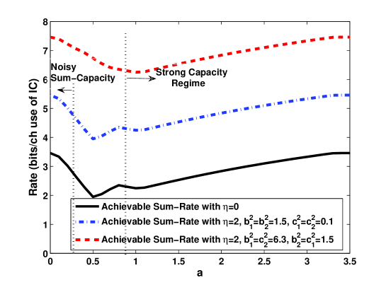
Figure 2: Achievable sum-rate from Proposition 2 for IC-OBR Type-I with symmetric IC, for fixed OBRC bandwidth allocation versus $a$ for various OBRC link capacities, namely i) $\eta=0$ (no relay), ii) $\eta_{1R}=\eta_{2R}=\eta_{R1}=\eta_{R2}=1$, $b_{1}^{2}=b_{2}^{2}=1.5$, $c_{1}^{2}=c_{2}^{2}=0.3$, (which satisfies the conditions in Proposition 3), and iii) $\eta_{1R}=\eta_{2R}=\eta_{R1}=\eta_{R2}=1$, $b_{2}^{2}=c_{1}^{2}=6.3$, $b_{1}^{2}=c_{2}^{2}=1.5$ (which satisfies the conditions in Proposition 4). All powers are set to $10$ dB.

In Fig. 2, we show the maximum achievable sum-rate of Proposition 2 for different configurations of the OBRC channel gains and bandwidths. We have a symmetric IC with $P=P_{1}=P_{2}=10$dB and $a_{21}=a_{12}=a$. For comparison, we show the no relay case $\eta_{1R}=\eta_{2R}=\eta_{R1}=\eta_{R2}=0$. Moreover, we first consider a scenario where the relay-to-destination links form bottleneck with respect to source-to-relay links, i.e. $\eta_{1R}\mathcal{C}(b_{1}^{2}P_{1R})=\eta_{2R}\mathcal{C}(b_{2}^{2}P_{2R})=2,\eta_{R1}\mathcal{C}(c_{1}^{2}P_{R1})=\eta_{R2}\mathcal{C}(c_{2}^{2}P_{R2})=1,$ thus falling within the assumptions of Proposition 3. It can be seen that the sum-rate increases by $2$ bits/ch use of IC for all values of $a$. Moreover, from Proposition 3, it is known that in the noisy [35] $\left(a(1+10a^{2})\leq 0.5,\mbox{ i.e, }a\leq 0.28\right)$ and strong ($a\geq 1$) [7] interference regimes, the sum-rate shown in the figure is the sum-capacity. Finally, we consider a situation with $\eta_{2R}\mathcal{C}(b_{2}^{2}P_{2R})=\eta_{R1}\mathcal{C}(c_{1}^{2}P_{R1})=3,\eta_{1R}\mathcal{C}(b_{1}^{2}P_{1R})=\eta_{R2}\mathcal{C}(c_{2}^{2}P_{R2})=2,$ which falls under the conditions of Proposition 4 for $a\geq 1$. As stated in the Proposition, for $a\geq 1$, the sum-rate shown in the sum-capacity is $4$ bits/channel use of IC larger than the reference case of zero OBRC capacities.

Proposition 5 (Excess rate regime, Mixed interference): For an IC-OBR Type-I with fixed OBRC bandwidth allocation and the condition $a_{12}<1$, we have that if $R_{ex_{21}}\geq\max\left\{0,\mathcal{C}(P_{1})+\mathcal{C}\left(\frac{P_{2}}{1+a_{12}^{2}P_{1}}\right)-\mathcal{C}\left(P_{1}+a_{21}^{2}P_{2}\right)\right\}$, the following condition characterizes the sum capacity

$$R_{1}+R_{2}\leq\mathcal{C}\left(P_{1}\right)+\mathcal{C}\left(\frac{P_{2}}{1+a_{12}^{2}P_{1}}\right)+\eta_{1R}\mathcal{C}(b_{1}^{2}P_{1R})+\eta_{R2}\mathcal{C}(c_{2}^{2}P_{R2}),$$

which is achieved by joint signal relaying and interference forwarding.

Proof: Appendix D.

Remark 4: Since $D_{2}$ observes weak interference, the optimal coding strategy for $S_{1}$ is to transmit private messages only, separably over both IC and OBRC. As for Proposition 4, interference forwarding essentially drives $D_{2}$ in a strong interference regime (even though we do not have $a_{21}\geq 1$ in general). Therefore, $S_{2}$ transmits only common messages in a non-separable way over both IC and OBRC via interference forwarding. It is also noted, similar to Remark 3, that if the interference at $D_{2}$ is strong enough on the IC, and in particular, we have

$$a_{21}\geq\sqrt{\frac{1+P_{1}}{1+a_{12}^{2}P_{1}}},$$ (18)

then it can be shown that interference forwarding is not necessary and one can set $R_{2c^{\prime}}=0$.

III-E Capacity Results for OBRC Variable Bandwidth Allocation

In this part, we discuss optimality of the considered strategies under variable OBRC bandwidth allocation. The next proposition shows that, thanks to the ability to allocate bandwidth among the source-to-relay and relay-to-destination channels, under certain conditions bandwidth can be allocated only to the best channels and in a way that only signal relaying is used.

Proposition 6: Consider an IC-OBR Type-I channel with variable OBRC bandwidth allocation and $a_{12}=a_{21}\geq 1$, $P_{1}=P_{2}$, $\mathcal{C}(b_{1}^{2}P_{1R})=\mathcal{C}(c_{1}^{2}P_{R1})$, $\mathcal{C}(b_{1}^{2}P_{1R})\geq\mathcal{C}(b_{2}^{2}P_{2R})$ and $\mathcal{C}(c_{1}^{2}P_{R1})\geq 2\mathcal{C}(c_{2}^{2}P_{R2})$. The sum capacity is given by

$$R_{1}+R_{2}\leq\mathcal{C}\left(a_{12}^{2}P_{1}+P_{2}\right)+\frac{\eta}{2}\mathcal{C}(c_{1}^{2}P_{R1})$$

and is achieved by signal relaying and transmitting only common information on the IC.

Proof: Appendix E.

Remark 5: Proposition 6 states that for a symmetric and strong IC, when the path $S_{1}-R-D_{1}$ is better than $S_{2}-R-D_{2}$ (see conditions on $b_{i}$ and $c_{i}),$ under appropriate conditions, it is optimal to allocate all the bandwidth $\eta$ to the better path to perform signal relaying. Signal relaying increases the sum-rate by the number of bits carried on the OBRC links, namely $\frac{\eta}{2}\mathcal{C}(c_{1}^{2}P_{R1}).$ Notice that it is possible to generalize Proposition 6 to arbitrary $b_{1}$ and $c_{1}$, i.e. not necessarily restricting the channels to satisfy the condition $\mathcal{C}(b_{1}^{2}P_{1R})=\mathcal{C}(c_{1}^{2}P_{R1})$. However, here we have focused on this simple case, to illuminate more clearly the gist of the main result.

To obtain further insight into the result of Proposition 6, in Fig. 3 we compare the sum-rate achievable by transmitting only common information on the IC and using signal relaying (with optimized bandwidth allocation), obtained from Proposition 2 (see (E. Proof of Proposition 6) in Appendix E), and the upper bound obtained from Proposition 1 (see (E. Proof of Proposition 6) in Appendix E). Parameters are fixed as $\eta=1$, $a_{21}=a_{12}=2$, $c_{1}=3,c_{2}=b_{2}=2,$ all powers equal to $10$ dB and $b_{1}$ is varied. Numerical results show for this example that the achievable rate matches the upper bound for most of the channel gains (except $1.2\leq b_{1}\leq 1.8$).

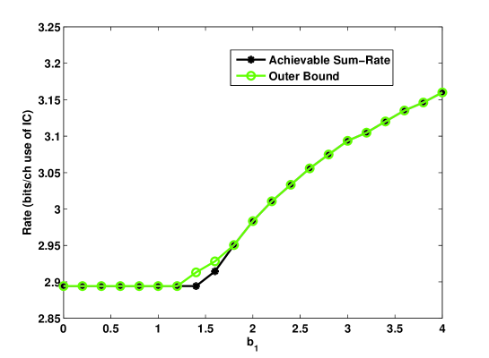
Figure 3: Achievable sum-rate (from Proposition 2, (E. Proof of Proposition 6) with signal relaying (only common information transmission over the IC), and outer bound (from Proposition 1, (E. Proof of Proposition 6)) versus $b_{1}$ for IC-OBR Type-I with variable OBRC bandwidth allocation ($\eta=1$, $a_{21}=a_{12}=2$, all powers equal to $10$ dB, $c_{1}=3,c_{2}=b_{2}=2)$.

The result in Proposition 6 begs the question as to whether interference forwarding can be ever useful in the case of variable bandwidth allocation. The following example answers this question in the affirmative. Consider an IC-OBR Type-I channel with $b_{1}=1.5$, $c_{1}=3$, $c_{2}=1$, $a_{12}=3$, $a_{21}=2,$ $\eta=1$ and all transmission powers set to $10$ dB. Here, $b_{2}$ is varied. Fig. 4 shows the achievable sum-rate obtained from Proposition 4 (which was derived from Proposition 2) by assuming transmission of common messages only over the IC and either signal relaying only ($(W_{ic^{\prime\prime}},W_{iR})$, $i=1,2$) or both signal relaying and interference forwarding ($(W_{1c^{\prime\prime}},W_{1R})$,$(W_{2c^{\prime}},W_{2c^{\prime\prime}},W_{2R})$) (see (52)-(55) in Appendix C) along with optimized bandwidth allocation ($\eta_{iR},\eta_{Ri}),$ $i=1,2$. Also shown is the outer bound from Proposition 1, given in (E. Proof of Proposition 6) for the channel parameters at hand. For $b_{2}\geq c_{2}=1$ and for fixed and equal bandwidth allocations, $\eta_{1R}=\eta_{R1}=\eta_{2R}=\eta_{R2}$, the excess rate $R_{ex_{21}}$ is positive and interference forwarding is potentially useful as discussed in Propositions 4. For the variable bandwidth case, Fig. 4 shows similarly that interference-forwarding is instrumental in improving the achievable sum-rate for $b_{2}\geq 2$. However, for $b_{2}<2$, interference forwarding is not needed.

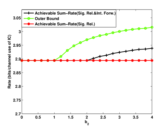
Figure 4: Achievable sum-rate (from Proposition 4, (52)-(55)) with signal relaying and interference forwarding (only common information transmission over the IC) and outer bound (from Proposition 1, (E. Proof of Proposition 6)) versus $b_{2}$ for IC-OBR Type-I with variable OBRC bandwidth allocation $\sum_{i=1}^{2}\eta_{iR}+\eta_{Ri}=\eta,$ $\eta=1$, $a_{12}=3$, $a_{21}=2$, all powers equal to $10$ dB, $b_{1}=1.5$, $c_{1}=3$, and $c_{2}=1$.

IV Analysis of IC-OBR Type-II

In this section, we investigate the IC-OBR Type-II channel described in Sec. II. This channel differs from IC-OBR Type-I in that on the OBRC: (i) The signals transmitted from $S_{1}$ and $S_{2}$ are superimposed at the relay; (ii) Relay broadcasts to the destinations. These aspects allow novel, and more general, transmission strategies at sources and relay, thus making the design of optimal schemes more complex than on the IC-OBR Type-I. This is reflected by the results presented below that encompass scenarios and techniques that have a counterpart in the IC-OBR Type-I analysis and others that stand out as specific to IC-OBR Type-II.

To simplify the analysis, we still consider the same class of strategies described in Sec. III-B for source and destinations. Namely, we assume a four-way message split into two private and two common parts, such that, as discussed in Remark 1, private signals are transmitted in a separable way over IC and OBRC, while one of the common messages is sent over both IC and OBRC (and, hence, transmitted in a non-separable way). Even within this class of strategies, the variety of possible approaches is remarkable. For instance, the relay may perform Decode-and-Forward (DF) or different flavors of Compress-and-Forward (CF) [26][27] and the sources may encode by using random codes or structured (e.g., lattice) codes [28][29]. For this reason, unlike IC-OBR Type-I, we will not give a general achievable rate region but rather focus on specific conditions under which optimality of certain design choices can be assessed.

We first give an outer bound on the capacity region for IC-OBR Type-II. Then, we investigate conditions under which signal relaying (and thus separable operation, as per the discussion above) or joint signal relaying/ interference forwarding (and thus non-separable strategies) are optimal.

IV-A Outer Bound

In the following, we give an outer bound that is the counterpart of Proposition 1 for IC-OBR Type-II.

Proposition 7 (Outer Bound for IC-OBR Type-II): For an IC-OBR Type-II with fixed OBRC bandwidth allocation, the capacity region is included in the following region

$$\lim_{n\rightarrow\infty}\mbox{closure}\bigg{(}\bigcup_{p(x_{1}^{n},x_{2}^{n})=p(x_{1}^{n})p(x_{2}^{n})}\big{\{}(R_{1},R_{2})\text{:}$$

$$R_{1} \leq\frac{1}{n}I(X_{1}^{n};Y_{1}^{n})+\eta_{MAC}\mathcal{C}\left(b_{1}^{2}P_{1R}+b_{2}^{2}P_{2R}\right)$$ (19a)

$$R_{1} \leq\frac{1}{n}I(X_{1}^{n};Y_{1}^{n}|X_{2}^{n})+\eta_{MAC}\mathcal{C}\left(b_{1}^{2}P_{1R}\right)$$ (19b)

$$R_{1} \leq\frac{1}{n}I(X_{1}^{n};Y_{1}^{n}|X_{2}^{n})+\eta_{BC}\mathcal{C}\left(c_{1}^{2}P_{R}\right)$$ (19c)

$$R_{2} \leq\frac{1}{n}I(X_{2}^{n};Y_{2}^{n})+\eta_{MAC}\mathcal{C}\left(b_{1}^{2}P_{1R}+b_{2}^{2}P_{2R}\right)$$ (19d)

$$R_{2} \leq\frac{1}{n}I(X_{2}^{n};Y_{2}^{n}|X_{1}^{n})+\eta_{MAC}\mathcal{C}\left(b_{2}^{2}P_{2R}\right)$$ (19e)

$$R_{2} \leq\frac{1}{n}I(X_{2}^{n};Y_{2}^{n}|X_{1}^{n})+\eta_{BC}\mathcal{C}\left(c_{2}^{2}P_{R}\right)\big{\}}\bigg{)}$$ (19f)

where the union is taken with respect to multi-letter input distributions $$p(x_{1}^{n})p(x_{2}^{n}) 1/n\sum_{t=1}^{n}\mbox{E}[X_{i,t}^{2}]\leq P_{i} i=1,2 a_{12}\leq 1 c_{1}\geq c_{2},$$ that satisfy the power constraints , . Moreover, if and the capacity region is included in a region given as above but with

$$R_{1} \leq\frac{1}{n}I(X_{1}^{n};Y_{1}^{n}|X_{2}^{n})+\eta_{BC}\mathcal{C}(c_{1}^{2}\xi P_{R})$$ (20)

$$R_{2} \leq\frac{1}{n}I(X_{2}^{n};Y_{2}^{n})+\eta_{BC}\mathcal{C}\left(\frac{c_{2}^{2}\overline{\xi}P_{R}}{1+c_{2}^{2}\xi P_{R}}\right)$$ (21)

instead of (19c) and (19f), respectively, and the union is taken also with respect to parameter $\xi,$ with $0\leq\xi\leq 1$ and $\overline{\xi}=1-\xi.$

With variable OBRC bandwidth allocation, an outer bound is given as above but with the union taken also with respect to all parameters $\eta_{MAC},\eta_{BC}$, $i=1,2,$ such that $\eta_{MAC}+\eta_{BC}$ $=\eta$.

Proof: Appendix F.

IV-B Review of Capacity Results

While, as explained above, the analysis of the IC-OBR Type-II is more complex than that of IC-OBR Type-I, we are able to identify specific sets of conditions on the OBRC and IC under which conclusive results can be found. Here we review such results.

We proceed as for the IC-OBR Type-I and consider at first R-to-D bottleneck conditions, akin to (10), which in this case reduce to

$$\eta_{MAC}\mathcal{C}(b_{1}^{2}P_{1R})\geq\eta_{BC}\mathcal{C}(c_{1}^{2}P_{R})\text{ and }c_{1}\geq c_{2},$$ (22)

or symmetrically by swapping indices 1 and 2. These conditions imply that the capacity region of the BC beween $R$ and $D_{1},D_{2}$ is completely included in the MAC capacity region between $S_{1},S_{2}$ and $R,$ as shown in Fig. 5. We show that, under appropriate channel conditions on the IC, the sum-capacity is obtained by signal relaying only (separable operation) in Proposition 8, similarly to Proposition 3 for IC-OBR Type-I.

We then consider a number of scenarios where the condition above is not satisfied, and an excess rate between $S_{2}$ and $D_{1}$, similar to (11), is available on the OBRC (see Fig. 6 for an illustration). We first show in Proposition 9 that, similarly to Proposition 4 and 5 (see Remarks 3 and 4), if decoder $D_{2}$ is already in sufficiently strong interference conditions, then interference forwarding is not necessary. We then exhibit a set of conditions under which interference forwarding, along with signal relaying, achieves capacity in Proposition 10. This result is akin to Proposition 5 in that it mimics the sum-capacity result for a Gaussian IC in the mixed-interference regime, and the excess rate on the OBRC has the effect of driving decoder $D_{2}$ in the strong interference regime. While the two results above are obtained via DF on the OBRC, we finally show that CF may be optimal too in Proposition 11.

We then consider variable bandwidth allocation over the OBRC and obtain, via numerical results, similar conclusions as for the type-I IC-OBR.

IV-C Capacity Results for Fixed OBRC Bandwidth Allocation

In this section, we consider fixed OBRC bandwidth allocation.

IV-C1 R-to-D Bottleneck Regime

The next Proposition finds the sum-capacity for the R-to-D bottleneck regime (22).

Proposition 8 (R-to-D Bottleneck Regime): In an IC-OBR Type-II with fixed bandwidth allocation and (22), we have that if $a_{12}<1$, $a_{21}\geq\sqrt{\frac{1+P_{1}}{1+a_{12}^{2}P_{1}}}$, the sum capacity is given by

$$R_{1}+R_{2}\leq\mathcal{C}\left(P_{1}\right)+\mathcal{C}\left(\frac{P_{2}}{1+a_{12}^{2}P_{1}}\right)+\eta_{BC}\mathcal{C}\left(c_{1}^{2}P_{R}\right)$$ (23)

and is obtained by signal relaying only and separable operation.

Proof: Appendix G.

Figure 5: Illustration of the OBRC conditions leading to the sum-capacity in Proposition 8: $c_{1}\geq c_{2}$, $\eta_{MAC}\mathcal{C}(b_{1}^{2}P_{1R})\geq\eta_{BC}\mathcal{C}(c_{1}^{2}P_{R})$.

Figure 6: Illustration of the OBRC conditions leading to the sum-capacity in Proposition 9: $c_{1}\geq c_{2}$, $\eta_{MAC}\mathcal{C}(b_{1}^{2}P_{1R})<\eta_{BC}\mathcal{C}(c_{1}^{2}P_{R})$, $\eta_{MAC}\mathcal{C}\left(\frac{b_{2}^{2}P_{2R}}{1+b_{1}^{2}P_{1R}}\right)\geq\eta_{BC}C\left(\frac{c_{2}^{2}\overline{\xi}^{\ast}P_{R}}{1+c_{2}^{2}\xi^{\ast}P_{R}}\right)$ where where $\xi^{\ast}$ is the optimal power allocation that maximizes the sum-rate in Proposition 12 ($\overline{\xi}^{\ast}=1-\xi^{\ast})$.

Remark 6: In Proposition 8, the interference conditions on the IC are mixed and the optimal transmission strategy over the IC turns out to prescribe transmission of only private information by $S_{1}$ (given that $D_{2}$ is in weak interference) and of only common information by $S_{2}$ (given that $D_{1}$ is in a strong interference condition). The conditions on the OBRC are illustrated in Fig. 5. The optimal operation over the OBRC in terms of sum-rate is for only user 1 to transmit over the OBRC using signal forwarding with DF at the relay. Notice that this operating point on the OBRC (see dot in Fig. 5) is sum-rate optimal if one focuses on the OBRC alone and on DF, since the corresponding achievable rate region is given by the intersection of the MAC and BC regions in Fig. 5. Proposition 8 shows that such operating point is also optimal for communications over the IC-OBR under the given conditions.

IV-C2 Excess Rate Regime

We now consider the case where the R-to-D bottleneck condition $\eta_{MAC}\mathcal{C}(b_{1}^{2}P_{1R})\geq\eta_{BC}\mathcal{C}(c_{1}^{2}P_{R})$ is not satisfied.

Proposition 9 (Excess rate regime, Mixed Interference): In an IC-OBR Type-II with fixed bandwidth allocation, we have that if $a_{12}<1$, $a_{21}\geq\sqrt{\frac{1+P_{1}}{1+a_{12}^{2}P_{1}}},$ then the sum-capacity is given by

$$R_{1}+R_{2} \leq\max_{0\leq\xi\leq 1}\bigg{\{}\mathcal{C}\left(P_{1}\right)+\mathcal{C}\left(\frac{P_{2}}{1+a_{12}^{2}P_{1}}\right)+\min\big{\{}\eta_{MAC}\mathcal{C}\left(b_{1}^{2}P_{1R}\right),\eta_{BC}\mathcal{C}\left(c_{1}^{2}\xi P_{R}\right)\big{\}}$$

$$+\eta_{BC}\mathcal{C}\left(\frac{c_{2}^{2}\overline{\xi}P_{R}}{1+c_{2}^{2}\xi P_{R}}\right)\bigg{\}},$$ (24)

if

$$\eta_{MAC}\mathcal{C}(b_{1}^{2}P_{1R})<\eta_{BC}\mathcal{C}(c_{1}^{2}P_{R})\text{ and }\eta_{MAC}\mathcal{C}\left(\frac{b_{2}^{2}P_{2R}}{1+b_{1}^{2}P_{1R}}\right)\geq\eta_{BC}C\left(\frac{c_{2}^{2}\overline{\xi}^{\ast}P_{R}}{1+c_{2}^{2}\xi^{\ast}P_{R}}\right),$$ (25)

where $\xi^{\ast}$ is the optimal power allocation that maximizes the sum-rate (24) with $\overline{\xi}^{\ast}=1-\xi^{\ast}$. The sum-capacity is obtained by DF and signal relaying alone.

Proof: Appendix H.

Remark 7: The conditions (25) are illustrated in Fig. 6. Observing Fig. 6 and recalling Propositions 4-5, one could guess that signal relaying is suboptimal under the conditions of Proposition 9. In fact, these conditions entail an excess rate between $S_{2}$ and $D_{1}$, since the maximum rate $S_{2}-R$ (i.e., $\eta_{MAC}\mathcal{C}(b_{2}^{2}P_{2R})$) is larger than the maximum rate $R-D_{2}$ (i.e., $\eta_{BC}\mathcal{C}(c_{2}^{2}P_{R})$), while the opposite is true for the path $S_{1}-R-D_{1}.$ The fact that such excess rate is not to be exploited for interference forwarding by the optimal scheme of Proposition 9 can be interpreted in light of Remarks 3 and 4, since the condition $a_{21}\geq\sqrt{\frac{1+P_{1}}{1+a_{12}^{2}P_{1}}},$ assumed in Proposition 9, already guarantees strong interference condition at $D_{1},$ and thus no need for interference forwarding. We also remark that the sum-rate optimal operation of the OBRC requires signal relaying for both sources, not just source 1 as above, and transmission over the OBRC at rates given by the operating point indicated in the figure. This rate pair is characterized by the power split $\xi^{\ast}$ in Proposition 9.

We next consider the case when a very large excess rate between $S_{2}$ and $D_{1}$ is present, i.e.,

$$b_{2},c_{1}\rightarrow\infty,$$ (26)

and show that interference forwarding may be useful to drive $D_{1}$ in the strong interference regime. The result is akin to Proposition 5 for IC-OBR Type-I.

Proposition 10 (Excess rate regime, Mixed Interference): In an IC-OBR Type-II with fixed bandwidth allocation, the following conditions give an achievable region

$$R_{1} \leq\mathcal{C}(P_{1})+\eta_{MAC}\mathcal{C}(b_{1}^{2}P_{1R})$$ (27a)

$$R_{2} \leq\mathcal{C}\left(\frac{P_{2}}{1+a_{12}^{2}P_{1}}\right)+\eta_{BC}\mathcal{C}\left(\frac{c_{2}^{2}\overline{\xi}P_{R}}{1+c_{2}^{2}\xi P_{R}}\right)$$ (27b)

$$R_{1}+R_{2} \leq\mathcal{C}(P_{1}+a_{21}^{2}P_{2})+\eta_{BC}\mathcal{C}(c_{1}^{2}\xi P_{R})+\eta_{BC}\mathcal{C}\left(\frac{c_{2}^{2}\overline{\xi}P_{R}}{1+c_{2}^{2}\xi P_{R}}\right)$$ (27c)

$$R_{1}+R_{2} \leq\mathcal{C}(P_{1}+a_{21}^{2}P_{2})+\eta_{MAC}\mathcal{C}(b_{1}^{2}P_{1R}+b_{2}^{2}P_{2R})$$ (27d)

with $$\xi+\overline{\xi}\leq 1 a_{12}<1$$ via DF and joint signal relaying and interference forwarding. Moreover, if (26) and , the sum-capacity is achieved by such scheme and given by

$$R_{1}+R_{2}\leq\mathcal{C}(P_{1})+\mathcal{C}\left(\frac{P_{2}}{1+a_{12}^{2}P_{1}}\right)+\eta_{MAC}\mathcal{C}(b_{1}^{2}P_{1R})+\eta_{BC}\mathcal{C}(c_{2}^{2}P_{R}).$$

Proof: Appendix I.

Remark 8: The scheme achieving (27a)-(27d) is based on transmitting only private information over the IC and OBRC (signal relaying) by $S_{1}$, due to the weak interference at $D_{2},$ while $S_{2}$ transmits common information over the IC and both common and private on the OBRC (joint signal relaying and interference forwarding). This scheme is shown to be sum-rate optimal if weak interference is seen at $D_{2}$ and a large “excess rate” (26) is available between $S_{2}$ and $D_{1}$ so as to essentially drive $D_{2}$ in the very strong interference regime.

To investigate the role of interference forwarding in a non-asymptotic regime, Fig. 7 shows the sum-rate obtained from (27a)-(27d), by assuming that source 2 either uses only signal relaying (i.e., $R_{2c^{\prime}}=0$ in the achievable region given in Appendix I) or also interference forwarding, and the sum-rate upper bound obtained from Proposition 7 and given in (104), Appendix G. The OBRC gains are set to $b_{1}=1$, $b_{2}=10$, $c_{2}=1$ and $c_{1}$ is varied, all node powers are equal to 10 dB and $\eta_{MAC}=\eta_{BC}=1$. We also have $a_{12}=0.5$ and $S_{2}-D_{1}$ channel gain takes the values $a_{21}\in\{0.1,0.9.1.8\}$. Note that for $a_{21}=1.8\geq\sqrt{\frac{1+P_{1}}{1+a_{12}^{2}P_{1}}}=1.78$ the conditions given in Proposition 8 are satisfied and signal relaying alone is optimal. For $a_{21}\in\{0.1,0.9\}\leq 1.78,$ the advantages of interference forwarding become substantial with increasing $c_{1}$, which is due to the fact that the $S_{2}-D_{1}$ pair can exploit more excess rate. The asymptotic optimality derived in Proposition 10 is here shown to be attained for finite values of $b_{2},c_{1}.$

Figure 7: Achievable sum-rate and outer bound for an IC-OBR Type-II with respect to $R-D_{1}$ channel gain, $c_{1}$ and $S_{2}-D_{1}$ channel gain $a_{21}\in\{0.1,0.9.1.8\}$ ($a_{12}=0.5$, $b_{1}=1$, $b_{2}=10$, $c_{2}=1$ and all node powers are equal to 10 dB).

Finally, we briefly show that signal relaying may be (asymptotically) optimal also in combination with CF at the relay.

Proposition 11 (Optimality of CF): In an IC-OBR Type-II with fixed bandwidth allocation, the following rates are achievable via signal relaying and CF at the relay:

$$R_{1} \leq\mathcal{C}(P_{1})+\eta_{MAC}C\left(\frac{b_{1}^{2}P_{1R}}{1+\sigma^{2}}\right)$$ (28a)

$$R_{2} \leq\mathcal{C}(P_{2})+\eta_{MAC}C\left(\frac{b_{2}^{2}P_{2R}}{1+\sigma^{2}}\right)$$ (28b)

$$R_{1}+R_{2} \leq\min\left\{\mathcal{C}(P_{1}+a_{21}^{2}P_{2}),\mathcal{C}(a_{12}^{2}P_{1}+P_{2})\right\}+\eta_{MAC}C\left(\frac{b_{1}^{2}P_{1R}+b_{2}^{2}P_{2R}}{1+\sigma^{2}}\right),$$ (28c)

where $$\sigma^{2}$$ satisfies

$$\sigma^{2}\geq\frac{1+b_{1}^{2}P_{1R}+b_{2}^{2}P_{2R}}{\min\left\{(1+c_{1}^{2}P_{R})^{\frac{\eta_{BC}}{\eta_{MAC}}},(1+c_{2}^{2}P_{R})^{\frac{\eta_{BC}}{\eta_{MAC}}}\right\}-1}.$$

The above provides the capacity region, given by (123a)-(123d), for $a_{12}\geq 1,$ $a_{21}\geq 1$ and $c_{1},c_{2}\rightarrow\infty.$

Proof: Appendix J.

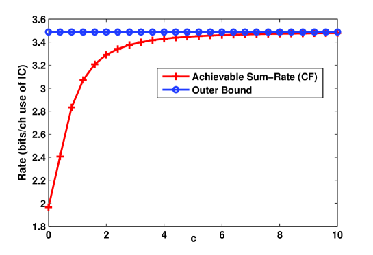
Figure 8: Achievable sum-rate ((28a)-(28c)) and outer bound ((123a)-(123d)) for an IC-OBR Type-II channel with symmetric IC and OBRC with respect to relay-to-destination channel gains, $c$ ($a=2$, $b=1,$ $P=P_{s}=10$ dB).

Remark 9: The rate (28a)-(28c) is achieved by transmitting common information over the IC, which leads to its optimality in the strong interference regime $a_{12}\geq 1,$ $a_{21}\geq 1$, and private information (signal relaying) over the OBRC. The relay performs CF which becomes optimal asymptotically as the relay-to-destination’s BC quality improves. Fig. 8 shows the comparison of achievable sum-rate obtained from (28a)-(28c) and the outer bound (123a)-(123d) on the sum-rate given in Proposition 11 from Appendix J for an IC-OBR Type-II channel with symmetric IC and OBRC as a function of $c$ with $a=2$, $b=1$, $P=P_{s}=10$ dB, $\eta=1$. We observe that the achievable sum-rate and outer bound are not only asymptotically equal for large $c,$ as shown by Proposition 11, but in practice become very close already for $c\geq 6$.

IV-D Capacity Results for OBRC Variable Bandwidth Allocation

Here, we briefly investigate the effect of variable bandwidth allocation for the IC-OBR Type-II via numerical results. We consider a mixed interference scenario with $a_{12}=0.5$, $a_{21}=1.8$ and $c_{1}\geq c_{2}$, which satisfies all the conditions of Proposition 8 except the ones that depend on the bandwidth allocation ($\eta_{MAC}$, $\eta_{BC}$). Recall that for given conditions on fixed allocations ($\eta_{MAC}$, $\eta_{BC}$), Proposition 8 shows the optimality of DF with signal relaying (separable operation). We compare the performance of the DF scheme in Proposition 8 (separable transmission) with an outer bound obtained from Proposition 7. In particular, from the conditions (19b) and (20) for $R_{1}$ and (19d) and (21) for $R_{2}$, with $a_{12}<1$, we obtain the following outer bound,

$$R_{1}+R_{2} \leq\mathcal{C}(P_{1})+\mathcal{C}\left(\frac{P_{2}}{1+a_{12}^{2}P_{1}}\right)+\min\left\{\eta_{MAC}\mathcal{C}(b_{1}^{2}P_{1R}),\eta_{BC}\mathcal{C}(c_{1}^{2}\xi P_{R})\right\}$$

$$+\min\left\{\eta_{MAC}C(b_{1}^{2}P_{1R}+b_{2}^{2}P_{2R}),\eta_{BC}C\left(\frac{c_{2}^{2}\overline{\xi}P_{R}}{1+c_{2}^{2}\xi P_{R}}\right)\right\}$$ (29)

for $\xi=1-\overline{\xi}$. In both cases, bandwidth allocation ($\eta_{MAC},\eta_{BC})$ is optimized.

In Fig. 9, the sum-rate discussed above are shown for variable $S_{1}-R$ gain, $b_{1}$, and the other channel gains are set to $b_{2}=2$, $c_{1}=2$, $c_{2}=0.3$ and all nodes powers are $10$ dB and $\eta=1$. The right part of the figure also shows the optimal bandwidth ($\eta_{MAC}$ and $\eta_{BC}$) and power ($\xi$) allocation. We know from Proposition 8 that if $b_{1}$ is sufficiently larger than $c_{1}$, for fixed bandwidth allocation, the DF rate (23) where the relay helps the $S_{1}-D_{1}$ pair only, is optimal. A similar conclusion is drawn here for $b_{1}\geq 2$ as it can be seen from the optimal power allocation $\xi$. Moreover, the total bandwidth is balanced between the $S_{1}-R$ and $R-D_{1}$ channels. This result is akin to Proposition 6 for IC-OBR Type-I.

Proposition 9 proves that, for fixed bandwidth allocation, if $c_{1}$ and $b_{2}$ are sufficiently large, it is optimal to use DF by letting the relay help both source-destination pairs. Fig. 10 shows that a similar conclusion holds also when optimizing the bandwidth allocation. Specifically, Fig. 10 compares the achievable sum-rate (24) (attained by the DF scheme just discussed) with the outer bound (IV-D) for variable $b_{1}$, and $b_{2}$, $c_{1}$ with values from the set $(b_{2},c_{1})\in\{(3,2),(10,5),(20,10)\}$. We also have $c_{2}=1$, $\eta={1}$, and other conditions as above. It is seen that for $(b_{2},c_{1})$ large enough, the outer bound and the achievable sum-rate match for $b_{1}\leq 7$.

A natural question that arises is to understand the effect of interference forwarding for IC-OBR Type-II with variable bandwidth allocation, similar to its IC-OBR Type-I counterpart as discussed in Sec. III-E. To observe this effect, we consider a Type-II channel with the parameters set to $\eta=1$, $a_{21}=1$, $a_{12}=0.5$, $c_{1}=4$, $c_{2}=1.5$, $b_{1}=1$, all powers equal to $10$ dB and $b_{2}$ is varied. Note that since $a_{21}\leq\sqrt{\frac{1+P_{1}}{1+a_{12}^{2}P_{1}}}=1.78$, $D_{1}$ can favor by the relay’s interference forwarding, since the interference can not be decoded and removed over the IC only at $D_{1}$ without affecting the sum-rate. Fig. 11 essentially shows that this is indeed the situation especially for $b_{2}\geq 2$. In the figure, the achievable scheme follows from Proposition 10, (27a)-(27d), where $S_{1}$ transmits only private information $W_{1p}$ via the IC whereas $S_{2}$ transmits common information $(W_{2c^{\prime}},W_{2c^{\prime\prime}})$ only. The relay facilitates interference forwarding by broadcasting $W_{2c^{\prime}}$ which is used at $D_{1}$ to remove part of the interference. As shown in the figure, the increase in $b_{2}$ gain helps the OBR forward more interference to $D_{1}$, and hence interference forwarding is crucial for larger $b_{2}$ gains.

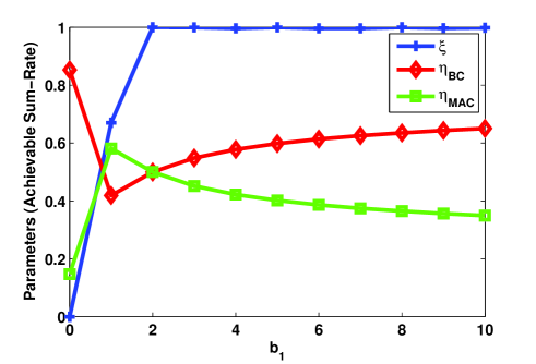
Figure 9: Achievable sum-rate (from Proposition 8, (23)) with signal relaying (DF) and outer bound (IV-D) and optimal parameters ($\eta_{MAC}$, $\eta_{BC}$, $\xi$) of the DF scheme (23) for an IC-OBR Type-II with respect to $S_{1}-R$ channel gain $b_{1}$ ($b_{2}=2$, $c_{1}=2$, $c_{2}=0.3$, $\eta={1}$, all node powers are equal to $10$ dB, $a_{21}=1.8$, $a_{12}=0.5.)$

Figure 10: Achievable sum-rate (from Proposition 8, (23)) with signal relaying (DF) and outer bound (IV-D) for an IC-OBR Type-II with respect to $S_{1}-R$ channel gain, $b_{1}$ and $(b_{2},c_{1})\in\{(3,2),(10,5),(20,10)\}$ ($c_{2}=1$, $\eta_{MAC}+\eta_{BC}=\eta$ with $\eta={1}$, all node powers are equal to $10$ dB, $a_{21}=1.8$, $a_{12}=0.5.)$

Figure 11: Achievable sum-rate (from Proposition 10, (27a)-(27d)) with signal relaying and interference forwarding (DF, only common information transmission by $S_{2}$ and only private information transmission by $S_{1}$ over the IC) and outer bound (IV-D) versus $b_{2}$ for IC-OBR Type-II with variable OBRC bandwidth allocation $\eta_{MAC}+\eta_{BC}=\eta,$ ($\eta=1$, $a_{21}=1$, $a_{12}=0.5$, all powers equal to $10$ dB, $c_{1}=4$, $c_{2}=1.5$, $b_{1}=1)$.

V Concluding Remarks

Operation over parallel radio interfaces is bound to become increasingly common in wireless networks due to the large number of multistandard terminals. This enables cooperation among terminals across different bandwidths and possibly standards. In this paper, we have studied one such scenario where two source-destination pairs, interfering over a given bandwidth, cooperate with a relay over an orthogonal spectral resource (out-of-band relaying, OBR). We have focused on two different models that correspond to distinct modes of transmission over the out-of-band relay channel (OBRC).

As discussed in previous work, relaying can assist interfering communications via standard signal relaying but also through interference forwarding, which eases interference mitigation. For both considered models, this paper has derived analytical conditions under which either signal relaying or interference forwarding are optimal. These conditions have also been related to the problem of assessing optimality of either separable or non-separable transmission over parallel interference channels. Overall, the analysis shows that, in general, joint signal relaying and interference forwarding, and thus non-separable transmission, is necessary to attain optimal performance. This clearly complicates the design. Moreover, this is shown to be the case for both fixed and variable (i.e., optimized) bandwidth allocation over the OBRC. However, in some special scenarios of interest, a separable approach has been shown to be optimal. An example of such cases, for both considered models, is the case where the relay has better channel conditions from the sources than to the destination (relay-to-destinations bottleneck regime). Moreover, in the presence of optimized OBRC bandwidth allocation, separable schemes are often (but not always) optimal.

The analysis in this paper leaves open a number of problems related to interference management via cooperation and through multiple radio interfaces. In particular, scenarios that extend the current model to more than two sources and one relay are of interest, and expected to offer new research challenges in light of the results of [33].

Appendix

A. Proof of Proposition 1

We consider outer bounds on $R_{1}$ and the bounds on $R_{2}$ can be obtained similarly. We have the following bound

$$nR_{1} =H(W_{1})$$ (30)

$$=I(W_{1};Y_{1}^{n},Y_{R1}^{\eta_{R1}n})+H(W_{1}|Y_{1}^{n},Y_{R1}^{\eta_{R1}n})$$ (31)

$$\leq I(W_{1};Y_{1}^{n},Y_{R1}^{\eta_{R1}n})+n\epsilon_{n}$$ (32)

$$\leq I(X_{1}^{n};Y_{1}^{n})+h(Y_{R1}^{\eta_{R1}n})-h(Z_{R1}^{\eta_{R1}n})+n\epsilon_{n},$$ (33)

where (32) follows from the Fano inequality $H(W_{1}|Y_{1}^{n},Y_{R1}^{\eta_{R1}n})\leq n\epsilon_{n}$ and (33) is from chain rule, the Markovity $W_{1}\rightarrow X_{1}^{n}\rightarrow Y_{1}^{n}$ and conditioning decreases entropy. Now, the first bound on $R_{1}$ in (8) can be obtained by noting that, $h(Y_{R1}^{\eta_{R1}n})-h(Z_{R1}^{\eta_{R1}n})=h(c_{1}X_{R1}^{\eta_{R1}n}+Z_{R1}^{\eta_{R1}n})-h(Z_{R1}^{\eta_{R1}n})$ $\leq n\eta_{R1}\mathcal{C}(c_{1}^{2}P_{R1})$, and therefore

$$nR_{1}\leq I(X_{1}^{n};Y_{1}^{n})+n\eta_{R1}\mathcal{C}(c_{1}^{2}P_{R1})+n\epsilon_{n}.$$

Also, from (32), we get the bound the other bound in (8) from the following series of inequalities

$$nR_{1} \leq I(W_{1};Y_{1}^{n},Y_{R1}^{\eta_{R1}n})+n\epsilon_{n}$$ (34)

$$\leq I(W_{1};Y_{1}^{n},Y_{1R}^{\eta_{1R}n},Y_{2R}^{\eta_{2R}n})+n\epsilon_{n}$$ (35)

$$\leq I(X_{1}^{n};Y_{1}^{n})+h(Y_{1R}^{\eta_{1R}n},Y_{2R}^{\eta_{2R}n})-h(Z_{1R}^{\eta_{1R}n})-h(Z_{2R}^{\eta_{2R}n})+n\epsilon_{n}$$ (36)

$$\leq I(X_{1}^{n};Y_{1}^{n})+h(Y_{1R}^{\eta_{1R}n})+h(Y_{2R}^{\eta_{2R}n})-h(Z_{1R}^{\eta_{1R}n})-h(Z_{2R}^{\eta_{2R}n})+n\epsilon_{n}$$ (37)

$$\leq I(X_{1}^{n};Y_{1}^{n})+n\eta_{1R}\mathcal{C}(b_{1}^{2}P_{1R})+n\eta_{2R}\mathcal{C}(b_{2}^{2}P_{2R})+n\epsilon_{n},$$ (38)

where (35) is from the Markov chain $W_{1}\rightarrow Y_{1R}^{\eta_{1R}n},Y_{2R}^{\eta_{2R}n}\rightarrow Y_{R1}^{\eta_{R1}n}$ and data processing inequality, (36) is from chain rule, $W_{1}\rightarrow X_{1}^{n}\rightarrow Y_{1}^{n}$ and conditioning decreases entropy and (37) is from independence of $Y_{1R}^{\eta_{1R}n}$ and $Y_{2R}^{\eta_{2R}n}$. Finally, the last bound on $R_{1}$ in (8) is obtained as,

$$nR_{1} =H(W_{1}|W_{2})$$ (39)

$$=I(W_{1};Y_{1}^{n},Y_{R1}^{\eta_{R1}n}|W_{2})+H(W_{1}|Y_{1}^{n},Y_{R1}^{\eta_{R1}n},W_{2})$$ (40)

$$\leq I(W_{1};Y_{1}^{n},Y_{R1}^{\eta_{R1}n}|W_{2})+n\epsilon_{n}$$ (41)

$$=I(W_{1};Y_{1}^{n}|W_{2})+I(W_{1};Y_{R1}^{\eta_{R1}n}|Y_{1}^{n},W_{2})+n\epsilon_{n}$$ (42)

$$\leq I(X_{1}^{n};Y_{1}^{n}|X_{2})+h(Y_{R1}^{\eta_{R1}n}|W_{2})-h(Z_{R1}^{\eta_{R1}n})+n\epsilon_{n}.$$ (43)

Now, since $h(Y_{R1}^{\eta_{R1}n}|W_{2})-h(Z_{R1}^{\eta_{R1}n})\leq h(Y_{R1}^{\eta_{R1}n})-h(Z_{R1}^{\eta_{R1}n})\leq n\eta_{R1}\mathcal{C}(c_{1}^{2}P_{R1})$, we have

$$nR_{1}\leq I(X_{1}^{n};Y_{1}^{n}|X_{2}^{n})+n\eta_{R1}\mathcal{C}(c_{1}^{2}P_{R1})+n\epsilon_{n}.$$

Moreover, following (42), we have,

$$nR_{1} \leq I(X_{1}^{n};Y_{1}^{n}|X_{2}^{n})+I(W_{1};Y_{1R}^{\eta_{1R}n},Y_{2R}^{\eta_{2R}n}|Y_{1}^{n},W_{2})+n\epsilon_{n}$$ (44)

$$\leq I(X_{1}^{n};Y_{1}^{n}|X_{2}^{n})+h(Y_{1R}^{\eta_{1R}n},Y_{2R}^{\eta_{2R}n}|W_{2})-h(Z_{1R}^{\eta_{1R}n})-h(Z_{2R}^{\eta_{2R}n})+n\epsilon_{n}$$ (45)

$$\leq I(X_{1}^{n};Y_{1}^{n}|X_{2}^{n})+h(Y_{1R}^{\eta_{1R}n})-h(Z_{1R}^{\eta_{1R}n})+n\epsilon_{n}$$ (46)

$$\leq I(X_{1}^{n};Y_{1}^{n}|X_{2}^{n})+n\eta_{1R}\mathcal{C}(b_{1}^{2}P_{1R})+n\epsilon_{n}$$ (47)

where (44) is from $W_{1}\rightarrow Y_{1R}^{\eta_{1R}n},Y_{2R}^{\eta_{2R}n}\rightarrow Y_{R1}^{\eta_{R1}n}$, (45) is due to conditioning decreases entropy and (46) is from the fact that $X_{2R}^{\eta_{2R}n}$ is a function of $W_{2}$ and independence of $Y_{1R}^{\eta_{1R}n}$ and $Z_{2R}^{\eta_{2R}n}$.

The general outer bound is then obtained by taking the union of all rates $(R_{1},R_{2})$ satisfying the constraints for all $n\geq 0$ and input distributions $p(x^{n}_{1},x^{n}_{2})=p(x^{n}_{1})p(x^{n}_{2})$, with power constraints $(P_{1},P_{2})$, which can be proved to coincide with the limiting region in (8), (see, e.g., [5], Remark 1). $\Box$

B. Proof of Proposition 2

Codeword Generation and Encoding: The sources divide their messages as $W_{1}=(W_{1R},W_{1p},W_{1c^{\prime}},W_{1c^{\prime\prime}})$, and $W_{2}=(W_{2R},W_{2p},W_{2c^{\prime}},W_{2c^{\prime\prime}})$ as explained in Sec.III-B. Messages $W_{ip}$ and ($W_{ic^{\prime}}$,$W_{ic^{\prime\prime}})$ are encoded into codewords $X_{ip}^{n}$ and $X_{ic}^{n}$ with rates $R_{ip}$, $R_{ic^{\prime}}+R_{ic^{\prime\prime}}$ for $i=1,2$, respectively, and sent over the IC in $n$ channel uses. Such codewords are generated i.i.d. from independent Gaussian distributions with zero-mean and powers $P_{ip},$ $P_{ic},$ respectively. Overall, we have the transmitted codewords over the IC:

$$X_{1}^{n}(W_{1}) =X_{1p}^{n}(W_{1p})+X_{1c}^{n}(W_{1c^{\prime}},W_{1c^{\prime\prime}})$$ (48a)

$$X_{2}^{n}(W_{2}) =X_{2p}^{n}(W_{2p})+X_{2c}^{n}(W_{2c^{\prime}},W_{2c^{\prime\prime}}).$$ (48b)

Message $$W_{iR} D_{i} S_{i} W_{ic^{{}^{\prime}}} D_{j} j\neq i, (W_{ic^{{}^{\prime}}},W_{iR}) S_{i} X_{iR}^{\eta_{iR}n}(W_{ic^{\prime}},W_{iR}) R_{ic^{\prime}}+R_{iR} P_{iR} i=1,2 (W_{1R},W_{2R},W_{1c^{\prime}},W_{2c^{\prime}}) X_{Ri}^{\eta_{Ri}n}(W_{jc^{\prime}},W_{iR}) R_{jc^{\prime}}+R_{iR} P_{Ri}, j\neq i i,j=1,2.$$ is transmitted to via the OBRC only. Moreover, to facilitate interference cancellation, source transmits message to the interfered destination , via the OBRC. The messages are jointly encoded by into the codewords which are generated i.i.d. with rate from independent Gaussian distributions with zero-mean and power , . On the other hand, after successfully decoding the messages , the OBR encodes these messages into the codewords with rate which are also generated i.i.d. from independent Gaussian distributions with zero-mean and power ,

Decoding: The destination $D_{i}$ initially decodes the messages $(W_{jc^{\prime}},W_{Ri})$ using the $R-D_{i}$ channel which leads to the achievable rates (9e) and (9f). The signals received on the IC are given by (1) with (48). Moreover, since the destination $D_{1}$ decodes $W_{2c^{\prime}}$, it thus sees an equivalent codebook $X_{2c}^{n}(W_{2c^{\prime}},W_{2c^{\prime\prime}})$ with only $2^{nR_{2c^{\prime\prime}}}$ codewords (and power $P_{ic}).$ Similarly, $D_{2}$ sees an equivalent codebook $X_{1c}^{n}(W_{1c^{\prime}},W_{1c^{\prime\prime}})$ with rate$\ R_{1c^{\prime\prime}}.$ Decoding of the messages $(W_{1c^{\prime}},W_{1c^{\prime\prime}},W_{1p},W_{2c^{\prime\prime}})$ at destination $D_{1}$ (and $(W_{2c^{\prime}},W_{2c^{\prime\prime}},W_{2p},W_{1c^{\prime\prime}})$ at destination $D_{2})$ is then performed jointly as over a multiple access channel with three sources of rates $R_{1c}=R_{1c^{\prime}}+R_{1c^{\prime\prime}},$ $R_{1p}$ and $R_{2c^{\prime\prime}}$ (and $R_{2c}=R_{2c^{\prime}}+R_{2c^{\prime\prime}},$ $R_{2p}$ and $R_{1c^{\prime\prime}}$ for $D_{2}$), by treating the private messages as noise, thus with equivalent noise power $N_{i}=a_{ji}^{2}P_{jp}+1$ for $i,j=1,2$, $i\neq j$ hence giving the achievable rates (9a) and (9b). It is also noted that, as explained in [17], error events corresponding to erroneous decoding of only message $W_{2c^{\prime\prime}}$ at destination $D_{1}$ and $W_{1c^{\prime\prime}}$ at destination $D_{2}$ do not contribute to the probability of error and thus can be neglected. The relay decodes the messages $(W_{ic^{\prime}},W_{iR})$, $i=1,2$ using the orthogonal source-to-relay links as given in (2). Therefore, it is possible to show that the rates in (9c) and (9d) which are the point-to-point rates in decoding the messages $(W_{iR},W_{ic^{\prime}})$ are achievable. $\Box$

C. Proof of Proposition 4

We start with part (i). The converse follows from Proposition 1. Namely, the upper bounds on individual rates (14a) and (14b) are a consequence of the second bounds on both $R_{1}$ and $R_{2}$, while the upper bound on the sum rate (14c) follows by summing second and first bounds on $R_{1}$, $R_{2}$, respectively and accounting for the condition $a_{12}\geq 1$ as

$$R_{1}+R_{2} \leq\frac{1}{n}I(X_{1}^{n};Y_{1}^{n}|X_{2}^{n})+\frac{1}{n}I(X_{2}^{n};Y_{2}^{n})+\min\left(\eta_{1R}\mathcal{C}(b_{1}^{2}P_{1R}),\eta_{R1}\mathcal{C}(c_{1}^{2}P_{R1}\right))$$

$$+\min\left(\eta_{1R}\mathcal{C}(b_{1}^{2}P_{1R})+\eta_{2R}\mathcal{C}(b_{2}^{2}P_{2R}),\eta_{R2}\mathcal{C}(c_{2}^{2}P_{R2})\right)$$ (49)

$$=\frac{1}{n}h(X_{1}^{n}+Z_{1}^{n})-h(Z_{1}^{n})+\frac{1}{n}h(a_{12}X_{1}^{n}+X_{2}^{n}+Z_{2}^{n})-\frac{1}{n}h(a_{12}X_{1}^{n}+Z_{2}^{n})$$

$$+\eta_{1R}\mathcal{C}(b_{1}^{2}P_{1R})+\eta_{R2}\mathcal{C}(c_{2}^{2}P_{R2})$$ (50)

$$\leq\mathcal{C}(a_{12}^{2}P_{1}+P_{2})+\eta_{1R}\mathcal{C}(b_{1}^{2}P_{1R})+\eta_{R2}\mathcal{C}(c_{2}^{2}P_{R2})$$ (51)

where (50) is due to the conditions $\eta_{1R}\mathcal{C}(b_{1}^{2}P_{1R})\leq\eta_{R1}\mathcal{C}(c_{1}^{2}P_{R1})$ and $\eta_{R2}\mathcal{C}(c_{2}^{2}P_{R2})\leq\eta_{2R}\mathcal{C}(b_{2}^{2}P_{2R})$, (51) is from the worst-case noise result [12], i.e., $h(X_{2}^{n}+Z_{2}^{n})-h(a_{21}X_{2}^{n}+Z_{1}^{n})\leq n\log(1)$ for $a_{21}\geq 1$, and the first entropy is maximized by i.i.d. Gaussian inputs.

For achievability, we use the general result of Proposition 2, where the sources transmit common messages $(W_{1c^{\prime\prime}},W_{2c^{\prime\prime}})$ over the IC which are decoded at both destinations. In addition, $S_{2}$ transmits also the message $W_{2c^{\prime}}$ to be decoded at $D_{2}$. The other rates are set to $R_{1c^{\prime}}=R_{1p}=R_{2p}=0.$ The OBRC is used to transmit independent messages $W_{1R},W_{2R}$ with rates $R_{1R}=\eta_{1R}\mathcal{C}(b_{1}^{2}P_{1R})$ and $R_{2R}=\eta_{R2}\mathcal{C}(c_{2}^{2}P_{R2})$, but also message $W_{2c^{\prime}}$ of rate $R_{2c^{\prime}}$ to $D_{1}$ in order to facilitate interference cancellation. From Proposition 2, and applying Fourier-Motzkin elimination, we obtain the following achievable region

$$R_{1} \leq\mathcal{C}(P_{1})+\eta_{1R}\mathcal{C}(b_{1}^{2}P_{1R})$$ (52)

$$R_{2} \leq\mathcal{C}(P_{2})+\eta_{R2}\mathcal{C}(c_{2}^{2}P_{R2})$$ (53)

$$R_{1}+R_{2} \leq\mathcal{C}(a_{12}^{2}P_{1}+P_{2})+\eta_{1R}\mathcal{C}(b_{1}^{2}P_{1R})+\eta_{R2}\mathcal{C}(c_{2}^{2}P_{R2})$$ (54)

$$R_{1}+R_{2} \leq\mathcal{C}(P_{1}+a_{21}^{2}P_{2})+R_{ex_{21}}+\eta_{1R}\mathcal{C}(b_{1}^{2}P_{1R})+\eta_{R2}\mathcal{C}(c_{2}^{2}P_{R2}),$$ (55)

so that for $R_{ex_{21}}$ $\geq$ $\max\{0,\mathcal{C}(a_{12}^{2}P_{1}+P_{2})-\mathcal{C}(P_{1}+a_{21}^{2}P_{2})\}$, the claim is proved.

We now move to part (ii). The converse is again a consequence of Proposition 1. Specifically, the single rate bounds (15) and (16) follow immediately from the second bounds on $R_{1}$ and $R_{2}$, while the bound on the sum-rate (14) is obtained from the summation of first and second bound on $R_{1}$, $R_{2}$, respectively, and the condition $a_{12}\geq 1$ as

$$R_{1}+R_{2} \leq\frac{1}{n}I(X_{1}^{n};Y_{1}^{n})+\frac{1}{n}I(X_{2}^{n};Y_{2}^{n}|X_{1}^{n})+\min(\eta_{1R}\mathcal{C}(b_{1}^{2}P_{1R})+\eta_{2R}\mathcal{C}(b_{2}^{2}P_{2R}),\eta_{R1}\mathcal{C}(c_{1}^{2}P_{R1}))$$

$$+\min(\eta_{2R}\mathcal{C}(b_{2}^{2}P_{2R}),\eta_{R2}\mathcal{C}(c_{2}^{2}P_{R2}))$$ (56)

$$=\frac{1}{n}h(X_{1}^{n}+a_{21}X_{2}^{n}+Z_{1}^{n})-\frac{1}{n}h(a_{21}X_{2}^{n}+Z_{1}^{n})+\frac{1}{n}h(X_{2}^{n}+Z_{2}^{n})-h(Z_{2}^{n})$$

$$+\eta_{R1}\mathcal{C}(c_{1}^{2}P_{R1})+\eta_{R2}\mathcal{C}(c_{2}^{2}P_{R2})$$ (57)

$$\leq\mathcal{C}(P_{1}+a_{21}^{2}P_{2})+\eta_{R2}\mathcal{C}(c_{2}^{2}P_{R2})+\eta_{R1}\mathcal{C}(c_{1}^{2}P_{R1}),$$ (58)

where (C. Proof of Proposition 4) is due to the conditions $\eta_{R1}\mathcal{C}(c_{1}^{2}P_{R1})+\eta_{R2}\mathcal{C}(c_{2}^{2}P_{R2})\leq\eta_{1R}\mathcal{C}(b_{1}^{2}P_{1R})+\eta_{2R}\mathcal{C}(b_{2}^{2}P_{2R})$ and $\eta_{R2}\mathcal{C}(c_{2}^{2}P_{R2})\leq\eta_{2R}\mathcal{C}(b_{2}^{2}P_{2R})$, (58) is from the worst-case noise result [12], i.e., $h(X_{2}^{n}+Z_{2}^{n})-h(a_{21}X_{2}^{n}+Z_{1}^{n})\leq n\frac{1}{2}\log(1)$ for $a_{21}\geq 1$, and the fact that first entropy is maximized by i.i.d. Gaussian inputs.

For the achievability, consider the achievable rate region given in the proof of Proposition 4 ((52)-(55)) (14a)-(14c). Clearly, when the conditions in Proposition 5 which can also be written as $\eta_{R1}\mathcal{C}(c_{1}^{2}P_{R1})-\eta_{1R}\mathcal{C}(b_{1}^{2}P_{1R})\leq\eta_{2R}\mathcal{C}(b_{2}^{2}P_{2R})-\eta_{R2}\mathcal{C}(c_{2}^{2}P_{R2})$ and $R_{ex_{21}}\leq\mathcal{C}(a_{12}^{2}P_{1}+P_{2})-\mathcal{C}(P_{1}a_{21}^{2}P_{2})$ are satisfied, (58) is achievable, hence gives the sum capacity. $\Box$

D. Proof of Proposition 5

The converse is obtained from Proposition 1 by adding the second constraint on $R_{1}$ and first constraint on $R_{2}$ in (8) such that,

$$R_{1}+R_{2} \leq\frac{1}{n}I(X_{1}^{n};Y_{1}^{n}|X_{2}^{n})+\frac{1}{n}I(X_{2}^{n};Y_{2}^{n})+\min(\eta_{1R}\mathcal{C}(b_{1}^{2}P_{1R}),\eta_{R1}\mathcal{C}(c_{1}^{2}P_{R1}))$$

$$+\min(\eta_{1R}\mathcal{C}(b_{1}^{2}P_{1R})+\eta_{2R}\mathcal{C}(b_{2}^{2}P_{2R}),\eta_{R2}\mathcal{C}(c_{2}^{2}P_{R2}))$$ (59)

$$=\frac{1}{n}h(X_{1}^{n}+Z_{1}^{n})-\frac{1}{n}h(Z_{1}^{n})+\frac{1}{n}h(a_{12}X_{1}^{n}+X_{2}^{n}+Z_{2}^{n})-\frac{1}{n}h(a_{12}X_{1}^{n}+Z_{2}^{n})$$

$$+\eta_{1R}\mathcal{C}(b_{1}^{2}P_{1R})+\eta_{R2}\mathcal{C}(c_{2}^{2}P_{R2})$$ (60)

$$\leq\mathcal{C}(P_{1})+\mathcal{C}\left(\frac{P_{2}}{1+a_{12}^{2}P_{1}}\right)+\eta_{1R}\mathcal{C}(b_{1}^{2}P_{1R})+\eta_{R2}\mathcal{C}(c_{2}^{2}P_{R2})$$ (61)

where (60) is due to the conditions $\eta_{R1}\mathcal{C}(c_{1}^{2}P_{R1})\geq\eta_{1R}\mathcal{C}(b_{1}^{2}P_{1R})$ and $\eta_{2R}\mathcal{C}(b_{2}^{2}P_{2R})\geq\eta_{R2}\mathcal{C}(c_{2}^{2}P_{R2})$, (61) is from the worst-case noise result of [12], i.e. $h(X_{1}^{n}+Z_{1}^{n})-h(a_{12}X_{1}^{n}+Z_{2}^{n})\leq n\mathcal{C}(P_{1})-n\mathcal{C}(a_{12}^{2}P_{1})$ for $a_{12}<1$.

Achievability follows directly from Proposition 2 by letting transmitter $S_{1}$ transmit private message only, i.e., $W_{1p}$ over the IC and $W_{1R}$ over the OBR, whereas user $S_{2}$ transmits common information both on the IC and OBR $(W_{2c^{\prime\prime}},W_{2c^{\prime}})$ as well as private message via OBR, $W_{2R}$. The other rates are set to zero $R_{1c^{\prime}}=R_{1c^{\prime\prime}}=R_{2p}=0$. Then, using Fourier-Motzkin elimination, it is possible to show that the following sum-rate is achievable,

$$R_{1}+R_{2} \leq\mathcal{C}(P_{1}+a_{21}^{2}P_{2})+R_{ex_{21}}+\eta_{1R}\mathcal{C}(b_{1}^{2}P_{1R})+\eta_{R2}\mathcal{C}(c_{2}^{2}P_{R2})$$ (62)

$$R_{1}+R_{2} \leq\mathcal{C}(P_{1})+\mathcal{C}\left(\frac{P_{2}}{1+a_{12}^{2}P_{1}}\right)+\eta_{1R}\mathcal{C}(b_{1}^{2}P_{1R})+\eta_{R2}\mathcal{C}(c_{2}^{2}P_{R2})$$ (63)

where $R_{ex_{21}}$ is given in (12). Then, for $R_{ex_{21}}\geq\mathcal{C}(P_{1})+\mathcal{C}\left(\frac{P_{2}}{1+a_{12}^{2}P_{1}}\right)-\mathcal{C}\left(P_{1}+a_{21}^{2}P_{2}\right)$, (63) is achievable, hence gives the sum capacity.$\Box$

E. Proof of Proposition 6

For the achievable scheme, we consider a special case of Proposition 2, where sources operate separately over the IC and OBRC, by sending only message $(W_{1R},W_{2R})$ over the OBRC (signal relaying) and only common information $(W_{1c^{\prime\prime}},W_{2c^{\prime\prime}})$ over the IC. From Proposition 2, i.e. using (9a)-(9f), we obtain that the following sum-rate is achievable

$$R_{1}+R_{2} \leq\mathcal{C}\left(a_{12}^{2}P_{1}+P_{2}\right)+\min\left\{\eta_{1R}\mathcal{C}(b_{1}^{2}P_{1R}),\eta_{R1}\mathcal{C}(c_{1}^{2}P_{R1}))\right\}$$

$$+\min\left\{\eta_{2R}\mathcal{C}(b_{2}^{2}P_{2R}),\eta_{R2}\mathcal{C}(c_{2}^{2}P_{R2}))\right\}$$ (64)

to be maximized over $(\eta_{iR},\eta_{Ri})$ with constraint $\sum_{i=1}^{2}(\eta_{iR}+\eta_{Ri})=\eta$. Optimizing over the bandwidth allocation, and recalling that $\mathcal{C}(b_{1}^{2}P_{1R})\geq\mathcal{C}(b_{2}^{2}P_{2R})$ and $\mathcal{C}(c_{1}^{2}P_{R1})\geq\mathcal{C}(c_{2}^{2}P_{R2})$, the optimal allocations are $\eta_{1R}^{\ast}=\eta_{R1}^{\ast}=\eta/2,$ so that the optimal achievable sum-rate is

$$R_{1}+R_{2}\leq\mathcal{C}\left(a_{12}^{2}P_{1}+P_{2}\right)+\frac{\eta\mathcal{C}(c_{1}^{2}P_{R1})}{2}.$$

For the outer bound, using Proposition 1 with $a_{12}=a_{21}\geq 1$, $P_{1}=P_{2}$, from (8), we obtain the upper bounds

$$R_{1}+R_{2} \leq\mathcal{C}\left(a_{12}^{2}P_{1}+P_{2}\right)+\min\{\eta_{1R}\mathcal{C}(b_{1}^{2}P_{1R})+\eta_{2R}\mathcal{C}(b_{2}^{2}P_{2R}),\eta_{R2}\mathcal{C}(c_{2}^{2}P_{R2})\}$$

$$+\min\{\eta_{1R}\mathcal{C}(b_{1}^{2}P_{1R}),\eta_{R1}\mathcal{C}(c_{1}^{2}P_{R1})\}$$ (65)

which should be maximized over $(\eta_{iR},\eta_{Ri})$ with $\sum_{i=1}^{2}(\eta_{iR}+\eta_{Ri})=\eta$. Optimizing over $(\eta_{iR},\eta_{Ri}),$ $i=1,2,$ using $\mathcal{C}(b_{1}^{2}P_{1R})\geq\mathcal{C}(b_{2}^{2}P_{2R})$, the optimal allocations satisfy, $\eta_{2R}^{*}=0$, $\eta_{1R}^{*}+\eta_{R1}^{*}+\eta_{R2}^{*}=\eta$, hence the optimization problem becomes,

$$R_{1}+R_{2} \leq\mathcal{C}\left(a_{12}^{2}P_{1}+P_{2}\right)+\min\{\eta_{1R}\mathcal{C}(b_{1}^{2}P_{1R}),\eta_{R2}\mathcal{C}(c_{2}^{2}P_{R2})\}$$

$$+\min\{\eta_{1R}\mathcal{C}(b_{1}^{2}P_{1R}),\eta_{R1}\mathcal{C}(c_{1}^{2}P_{R1})\}.$$ (66)

Since both $\min$ terms are limited by the same expression, $\eta_{1R}\mathcal{C}(b_{1}^{2}P_{1R})$, the optimal bandwidth allocation will lead to the largest among these two terms. On the other hand, optimizing the $\min$ terms individually, we have,

$$R_{1}+R_{2} \leq\max\bigg{\{}\mathcal{C}\left(a_{12}^{2}P_{1}+P_{2}\right)+\frac{2\eta\mathcal{C}(c_{1}^{2}P_{R1})\mathcal{C}(c_{2}^{2}P_{R2})}{\mathcal{C}(c_{1}^{2}P_{R1})+2\mathcal{C}(c_{2}^{2}P_{R2})},$$

$$\mathcal{C}\left(a_{12}^{2}P_{1}+P_{2}\right)+\frac{\eta\mathcal{C}(c_{1}^{2}P_{R1})}{2}\bigg{\}},$$ (67)

where the first term in the $\max$ corresponds to the choice $\eta_{R2}^{\ast}=\eta_{1R}^{\ast}\frac{\mathcal{C}(b_{1}^{2}P_{1R})}{\mathcal{C}(c_{2}^{2}P_{R2})},\mbox{ }\eta_{R1}^{\ast}=\eta_{1R}^{\ast},\mbox{ }\eta_{1R}^{\ast}+\eta_{R1}^{\ast}+\eta_{R2}^{\ast}=\eta,$ whereas the second to $\eta_{1R}^{\ast}=\eta_{R1}^{\ast}=\frac{\eta}{2},\eta_{R2}^{\ast}=0$. It is possible to show that for

$$\mathcal{C}(c_{1}^{2}P_{R1})\geq 2\mathcal{C}(c_{2}^{2}P_{R2})$$

the outer bound obtained in (67) becomes equal to the optimal achievable sum-rate.$\Box$

F. Proof of Proposition 7

We start with the bound (19a):

$$nR_{1} \leq H(W_{1})$$ (68)

$$\leq I(W_{1};Y_{1}^{n},Y_{R1}^{\eta_{BC}n})+H(W_{1}|Y_{1}^{n},Y_{R1}^{\eta_{BC}n})$$ (69)

$$\leq I(W_{1};Y_{1}^{n},Y_{R1}^{\eta_{BC}n})+n\epsilon_{n}$$ (70)

$$=I(W_{1};Y_{1}^{n})+I(W_{1};Y_{R1}^{\eta_{BC}n}|Y_{1}^{n})+n\epsilon_{n}$$ (71)

$$\leq I(X_{1}^{n};Y_{1}^{n})+I(W_{1};Y_{R}^{\eta_{MAC}n}|Y_{1}^{n})+n\epsilon_{n}$$ (72)

$$\leq I(X_{1}^{n};Y_{1}^{n})+h(Y_{R}^{\eta_{MAC}n})-h(Z_{R}^{\eta_{MAC}n})+n\epsilon_{n}$$ (73)

$$\leq I(X_{1}^{n};Y_{1}^{n})+h(b_{1}X_{1R}^{\eta_{MAC}n}+b_{2}X_{2R}^{\eta_{MAC}n}+Z_{R}^{\eta_{MAC}n})-h(Z_{R}^{\eta_{MAC}n})+n\epsilon_{n}$$ (74)

$$\leq I(X_{1}^{n};Y_{1}^{n})+\eta_{MAC}n\mathcal{C}\left(b_{1}^{2}P_{1R}+b_{2}^{2}P_{2R}\right)+n\epsilon_{n}$$ (75)

where (70) is from Fano’s inequality, (72) is from the Markov relations $W_{1}\rightarrow Y_{R}^{\eta_{MAC}n},Y_{1}^{n}\rightarrow Y_{R1}^{\eta_{BC}n}$ and $W_{1}\rightarrow X_{1}^{n}\rightarrow Y_{1}^{n}$.

From cut-set bound around $S_{1}$, we obtain the bound (19b) as

$$nR_{1} \leq I(X_{1}^{n};Y_{1}^{n}|X_{2}^{n})+I(X_{1R}^{\eta_{MAC}n};Y_{R}^{\eta_{MAC}n}|X_{2R}^{\eta_{MAC}n})$$ (76)

$$\leq I(X_{1}^{n};Y_{1}^{n}|X_{2}^{n})+\eta_{MAC}n\mathcal{C}\left(b_{1}^{2}P_{1R}\right).$$ (77)

Using similar steps we obtain the corresponding bounds on $R_{2}$ (19d) and (19e) as

$$nR_{2} \leq I(X_{2}^{n};Y_{2}^{n})+\eta_{MAC}n\mathcal{C}\left(b_{1}^{2}P_{1R}+b_{2}^{2}P_{2R}\right)$$ (78)

$$nR_{2} \leq I(X_{2}^{n};Y_{2}^{n}|X_{1}^{n})+\eta_{MAC}n\mathcal{C}\left(b_{2}^{2}P_{2R}\right).$$ (79)

We now focus on the bounds (20) and (21). For (21), we have (from (71) modified for $R_{2}$),

$$nR_{2} \leq I(X_{2}^{n};Y_{2}^{n})+I(W_{2};Y_{R2}^{\eta_{BC}n}|Y_{2}^{n})+n\epsilon_{n}$$ (80)

$$\leq I(X_{2}^{n};Y_{2}^{n})+h(Y_{R2}^{\eta_{BC}n})-h(c_{2}X_{R}^{\eta_{BC}n}+Z_{R2}^{\eta_{BC}n}|Y_{2}^{n},W_{2})+n\epsilon_{n}$$ (81)

where (81) is from conditioning decreases entropy. Now, consider the following,

$$h(Z_{R2}^{\eta_{BC}n})\leq h(c_{2}X_{R}^{\eta_{BC}n}+Z_{R2}^{\eta_{BC}n}|Y_{2}^{n},W_{2})\leq h(c_{2}X_{R}^{\eta_{BC}n}+Z_{R2}^{\eta_{BC}n})\leq\frac{\eta_{BC}n}{2}\log(2\pi e(1+c_{2}^{2}P_{R})).$$

Hence, without loss of generality, one can assume

$$h(Y_{R2}^{\eta_{BC}n}|Y_{2}^{n},W_{2})=\frac{\eta_{BC}n}{2}\log(2\pi e(1+c_{2}^{2}\xi P_{R})),$$ (82)

for some $0\leq\xi\leq 1$. Then, (81) becomes

$$nR_{2} \leq I(X_{2}^{n};Y_{2}^{n})+\frac{\eta_{BC}n}{2}\log(2\pi e(1+c_{2}^{2}P_{R}))-\frac{\eta_{BC}n}{2}\log(2\pi e(1+c_{2}^{2}\xi P_{R}))+n\epsilon_{n}$$ (83)

$$=I(X_{2}^{n};Y_{2}^{n})+\eta_{BC}n\mathcal{C}\left(\frac{c_{2}^{2}\overline{\xi}P_{R}}{1+c_{2}^{2}\xi P_{R}}\right)+n\epsilon_{n}$$ (84)

where we have used the fact that Gaussian distribution maximizes the entropy term for a given variance constraint.

Now, consider (70) for the bound on $R_{1}$ given in (20) which follows as,

$$nR_{1} \leq I(W_{1};Y_{1}^{n},Y_{R1}^{\eta_{BC}n}|W_{2})+n\epsilon_{n}$$ (85)

$$\leq I(X_{1}^{n};Y_{1}^{n}|X_{2}^{n})+I(W_{1};Y_{R1}^{\eta_{BC}n}|Y_{1}^{n},W_{2})+n\epsilon_{n}$$ (86)

$$=I(X_{1}^{n};Y_{1}^{n}|X_{2}^{n})+I(W_{1};\frac{c_{2}}{c_{1}}Y_{R1}^{\eta_{BC}n}|Y_{1}^{n},W_{2})+n\epsilon_{n}$$ (87)

where (85) is due to conditioning decreases entropy and independence of $W_{1}$ and $W_{2}$, (86) is from Markovity $W_{1}\rightarrow X_{1}^{n}\rightarrow Y_{1}^{n}$ and $X_{2}^{n}$ is a function of $W_{2}$, (87) is since scaling does not change the mutual information.

Since the capacity region of BC depends on the conditional marginal distributions and noting that $c_{1}\geq c_{2}$, we can write $Y_{R2}^{\eta_{BC}n}=\frac{c_{2}}{c_{1}}Y_{R1}^{\eta_{BC}n}+\widehat{Z}_{R}^{\eta_{BC}n}$ where $\widehat{Z}_{R}^{\eta_{BC}n}$ is an iid. Gaussian noise with variance $1-\frac{c_{2}^{2}}{c_{1}^{2}}$. From the conditional Entropy Power Inequality, we now have

$$2^{\frac{2}{\eta_{BC}n}h(Y_{R2}^{\eta_{BC}n}|Y_{1}^{n},W_{2})}\geq 2^{\frac{2}{\eta_{BC}n}h\left(\frac{c_{2}}{c_{1}}Y_{R1}^{\eta_{BC}n}|Y_{1}^{n},W_{2}\right)}+2^{\frac{2}{\eta_{BC}n}h\left(\widehat{Z}_{R}^{\eta_{BC}n}|Y_{1}^{n},W_{2}\right)}.$$ (88)

Also, for the condition $a_{12}\leq 1$, we have,

$$h(Y_{R2}^{\eta_{BC}n}|Y_{1}^{n},W_{2}) =h(Y_{R2}^{\eta_{BC}n}|X_{1}^{n}+Z_{1}^{n},W_{2})$$ (89)

$$=h(Y_{R2}^{\eta_{BC}n}|X_{1}^{n}+Z_{2}^{n},W_{2})$$ (90)

$$\leq h(Y_{R2}^{\eta_{BC}n}|a_{12}X_{1}^{n}+Z_{2}^{n},W_{2})$$ (91)

$$=h(Y_{R2}^{\eta_{BC}n}|Y_{2}^{n},W_{2})$$ (92)

$$=\frac{\eta_{BC}n}{2}\log(2\pi e(1+c_{2}^{2}\xi P_{R}))$$ (93)

where (89) is from the fact that $a_{21}X_{2}^{n}$ is a function of $W_{2}$, (90) follows from the independence of $Z_{R1}^{\eta_{BC}n}$, $Z_{1}^{n}$, and $Z_{2}^{n}$, (91) is due to the Markov chain, $a_{12}X_{1}^{n}+Z_{2}^{n}\rightarrow X_{1}^{n}+Z_{2}^{n},W_{2}\rightarrow Y_{R2}^{\eta_{BC}n}$ for the fact that $a_{12}\leq 1$, (92) is true since $X_{2}^{n}$ is a function of $W_{2}$, and (93) from (82). Then, using (88), (93), and noticing that $h\left(\widehat{Z}_{R}^{\eta_{BC}n}|Y_{1}^{n},W_{2}\right)=\frac{\eta_{BC}n}{2}\log\left(2\pi e(1-\frac{c_{2}^{2}}{c_{1}^{2}})\right)$, we obtain,

$$h\left(\frac{c_{2}}{c_{1}}Y_{R1}^{\eta_{BC}n}|Y_{1}^{n},W_{2}\right) \leq\frac{\eta_{BC}n}{2}\log\left(2\pi e\left(c_{2}^{2}\xi P_{R}+\frac{c_{2}^{2}}{c_{1}^{2}}\right)\right).$$ (94)

So that, recalling (87) and considering the inequality (94), we get,

$$nR_{1} \leq I(X_{1}^{n};Y_{1}^{n}|X_{2}^{n})+h(\frac{c_{2}}{c_{1}}Y_{R1}^{\eta_{BC}n}|Y_{1}^{n},W_{2})-h(\frac{c_{2}}{c_{1}}Z_{R1}^{\eta_{BC}n})+n\epsilon_{n}$$ (95)

$$\leq I(X_{1}^{n};Y_{1}^{n}|X_{2}^{n})+\eta_{BC}n\mathcal{C}\left(c_{1}^{2}\xi P_{R}\right)+n\epsilon_{n},$$ (96)

which recovers (20) and completes the proof.

Finally, we obtain the bound (19c) by continuing from (86)

$$nR_{1} \leq H(W_{1}|W_{2})$$ (97)

$$\leq I(W_{1};Y_{1}^{n},Y_{R1}^{\eta_{BC}n}|W_{2})+n\epsilon_{n}$$ (98)

$$\leq I(X_{1}^{n};Y_{1}^{n}|X_{2}^{n})+I(W_{1};Y_{R1}^{\eta_{BC}n}|Y_{1}^{n},W_{2})+n\epsilon_{n}$$ (99)

$$\leq I(X_{1}^{n};Y_{1}^{n}|X_{2}^{n})+h(Y_{R1}^{\eta_{BC}n})-h(Z_{R1}^{\eta_{BC}n})+n\epsilon_{n}$$ (100)

$$\leq I(X_{1}^{n};Y_{1}^{n}|X_{2}^{n})+n\eta_{BC}\mathcal{C}(c_{1}^{2}P_{R})+n\epsilon_{n}.$$ (101)

where (100) is true since conditioning decreases entropy and (101) is from the fact that Gaussian distribution maximizes the entropy for given variance constraints. Using similar steps, we obtain the rate for $R_{2}$ in (19f).$\Box$

G. Proof of Proposition 8

The converse follows from (19b), (20), and (21) as

$$R_{1}+R_{2} \leq\frac{1}{n}I(X_{1}^{n};Y_{1}^{n}|X_{2}^{n})+\frac{1}{n}I(X_{2}^{n};Y_{2}^{n})+\min\{\eta_{MAC}\mathcal{C}(b_{1}^{2}P_{1R}),\eta_{BC}\mathcal{C}(c_{1}^{2}\xi P_{R})\}$$

$$+\eta_{BC}\mathcal{C}\left(\frac{c_{2}^{2}\overline{\xi}P_{R}}{1+c_{2}^{2}\xi P_{R}}\right)$$ (102)

$$\leq\mathcal{C}(a_{12}^{2}P_{1}+P_{2})+\mathcal{C}(P_{1})-\mathcal{C}(a_{12}^{2}P_{1})$$

$$+\min\big{\{}\eta_{MAC}\mathcal{C}(b_{1}^{2}P_{1R}),\eta_{BC}\mathcal{C}(c_{1}^{2}\xi P_{R})\big{\}}+\eta_{BC}\mathcal{C}\left(\frac{c_{2}^{2}\overline{\xi}P_{R}}{1+c_{2}^{2}\xi P_{R}}\right)$$ (103)

$$=\mathcal{C}(P_{1})+\mathcal{C}\left(\frac{P_{2}}{1+a_{12}^{2}P_{1}}\right)+\min\big{\{}\eta_{MAC}\mathcal{C}(b_{1}^{2}P_{1R}),\eta_{BC}\mathcal{C}(c_{1}^{2}\xi P_{R})\big{\}}$$

$$+\eta_{BC}\mathcal{C}\left(\frac{c_{2}^{2}\overline{\xi}P_{R}}{1+c_{2}^{2}\xi P_{R}}\right)$$ (104)

where (G. Proof of Proposition 8) is from the worst-case noise result of [12] applied for $a_{12}\leq 1$. For $\eta_{MAC}\mathcal{C}(b_{1}^{2}P_{1R})\geq\eta_{BC}\mathcal{C}(c_{1}^{2}P_{R})$, (104) is maximized for $\xi=1$ since $c_{1}\geq c_{2}$, and hence the outer bound becomes

$$R_{1}+R_{2}\leq\mathcal{C}(P_{1})+\mathcal{C}\left(\frac{P_{2}}{1+a_{12}^{2}P_{1}}\right)+\eta_{BC}\mathcal{C}(c_{1}^{2}P_{R}).$$ (105)

For achievability, we use a special case of the coding scheme (48) in which, over the IC, $S_{1}$ transmits private information only via a Gaussian codebook $X_{1}^{n}(W_{1})=X_{1p}^{n}(W_{1p})$, and $S_{2}$ transmits common information using a Gaussian codebook $X_{2}^{n}(W_{2})=X_{2c}^{n}(W_{2c^{\prime\prime}})$. Only private messages ($W_{1R},W_{2R}$) are sent over the OBRC by using standard Gaussian codebooks and MAC decoding at the relay, and superposition coding at the relay. The proof then follows similarly to Proposition 2, Appendix B, by accounting for the capacity regions of MAC and BC Gaussian channels (see, e.g., [15]). Specifically, we obtain the following rates,

$$R_{1p} \leq\mathcal{C}(P_{1})$$ (106)

$$R_{2c} \leq\mathcal{C}\left(\frac{P_{2}}{1+a_{12}^{2}P_{1}}\right)$$ (107)

$$R_{1p}+R_{2c} \leq\mathcal{C}(P_{1}+a_{21}^{2}P_{2})$$ (108)

$$R_{1R} \leq\min\left\{\eta_{MAC}\mathcal{C}(b_{1}^{2}P_{1R}),\eta_{BC}\mathcal{C}\left(c_{1}^{2}\xi P_{1R}\right)\right\}$$ (109)

$$R_{2R} \leq\min\left\{\eta_{MAC}\mathcal{C}(b_{2}^{2}P_{2R}),\eta_{BC}\mathcal{C}\left(\frac{c_{2}^{2}\overline{\xi}P_{1R}}{1+c_{2}^{2}\xi P_{R}}\right)\right\}$$ (110)

$$R_{1R}+R_{2R} \leq\eta_{MAC}\mathcal{C}\left(b_{1}^{2}P_{1R}+b_{2}^{2}P_{2R}\right)$$ (111)

Then, setting $R_{1}=R_{1p}+R_{1R}$, $R_{2}=R_{2c}+R_{2R}$ with $\xi=1$, $\eta_{MAC}\mathcal{C}(b_{1}^{2}P_{1R})\geq\eta_{BC}\mathcal{C}(c_{1}^{2}P_{R})$ and $a_{21}\geq\sqrt{\frac{1+P_{1}}{1+a_{12}^{2}P_{1}}}$, the outer bound (105) is achievable, hence we obtain the sum capacity.

H. Proof of Proposition 9

The proof follows that in Appendix G. For $\eta_{MAC}\mathcal{C}(b_{1}^{2}P_{1R})<\eta_{BC}\mathcal{C}(c_{1}^{2}P_{R})$, denote $\xi^{\ast}$ as the optimal parameter that maximizes (104) so that we get

$$R_{1}+R_{2} \leq\mathcal{C}(P_{1})+\mathcal{C}\left(\frac{P_{2}}{1+a_{12}^{2}P_{1}}\right)+\min\big{\{}\eta_{MAC}\mathcal{C}(b_{1}^{2}P_{1R}),\eta_{BC}\mathcal{C}(c_{1}^{2}\xi^{\ast}P_{R})\big{\}}$$

$$+\eta_{BC}\mathcal{C}\left(\frac{c_{2}^{2}\overline{\xi}^{\ast}P_{R}}{1+c_{2}^{2}\xi^{\ast}P_{R}}\right)$$ (112)

where $\xi^{\ast}+\overline{\xi}^{\ast}=1$. Moreover, from (106)-(111), for the conditions $a_{21}\geq\sqrt{\frac{1+P_{1}}{1+a_{12}^{2}P_{1}}}$, $\eta_{MAC}\mathcal{C}(b_{1}^{2}P_{1R})<\eta_{BC}\mathcal{C}(c_{1}^{2}P_{R})$ and $\eta_{MAC}\mathcal{C}\left(\frac{b_{2}^{2}P_{2R}}{1+b_{1}^{2}P_{1R}}\right)\geq\eta_{BC}C\left(\frac{c_{2}^{2}\overline{\xi}^{\ast}P_{R}}{1+c_{2}^{2}\xi^{\ast}P_{R}}\right)$ and with the power split of $\xi^{\ast}P_{R}$ allocated at the relay for the transmission of $W_{1R}$ (and $\overline{\xi}^{\ast}P_{R}$ for $W_{2R}$), the achievable sum-rate obtained by $R_{1}=R_{1p}+R_{1R}$, $R_{2}=R_{2c}+R_{2R}$, is equal to the outer bound (H. Proof of Proposition 9).

VI I. Proof of Proposition 10

The achievable region is obtained similarly to Appendices B and G. Source $S_{1}$ transmits private message only, i.e., $X_{1}^{n}(W_{1})=X_{1p}^{n}(W_{1p})$ over the IC and independent private message over the OBRC $W_{1R}$ via Gaussian codebooks. Source $S_{2}$ transmits common messages $(W_{2c^{\prime}},W_{2c^{\prime\prime}})$ over the IC ($X_{2}^{n}(W_{2})=X_{2c}^{n}(W_{2c^{\prime}},W_{2c^{\prime\prime}})$), and the private message $W_{2R}$ is transmitted via the OBR along with $W_{2c^{\prime}}$ (interference forwarding). Then, the following conditions are easily seen to provide an achievable region

$$R_{1p} \leq\mathcal{C}(P_{1})$$ (113)

$$R_{2c^{\prime\prime}}+R_{1p} \leq\mathcal{C}(P_{1}+a_{21}^{2}P_{2})$$ (114)

$$R_{2c} \leq\mathcal{C}\left(\frac{P_{2}}{1+a_{12}^{2}P_{1}}\right)$$ (115)

$$R_{1R} \leq\eta_{MAC}\mathcal{C}(b_{1}^{2}P_{1R})$$ (116)

$$R_{2c^{\prime}}+R_{2R} \leq\eta_{MAC}\mathcal{C}(b_{2}^{2}P_{2R})$$ (117)

$$R_{1R}+R_{2c^{\prime}}+R_{2R} \leq\eta_{MAC}\mathcal{C}(b_{1}^{2}P_{1R}+b_{2}^{2}P_{2R})$$ (118)

$$R_{2c^{\prime}}+R_{1R} \leq\eta_{BC}\mathcal{C}(c_{1}^{2}\xi P_{R})$$ (119)

$$R_{2R} \leq\eta_{BC}\mathcal{C}\left(\frac{c_{2}^{2}\overline{\xi}P_{R}}{1+c_{2}^{2}\xi P_{R}}\right)$$ (120)

Using Fourier-Motzkin elimination method, with the fact that $R_{1}=R_{1p}+R_{1R}$, $R_{2c}=R_{2c^{\prime}}+R_{2c^{\prime\prime}}$, and $R_{2}=R_{2c}+R_{2R}$, the achievable region in Proposition 10 can be obtained. Now, for $b_{2},c_{1}\rightarrow\infty$, the achievable region becomes

$$R_{1} \leq\mathcal{C}(P_{1})+\eta_{MAC}\mathcal{C}(b_{1}^{2}P_{1R})$$ (121)

$$R_{2} \leq\mathcal{C}\left(\frac{P_{2}}{1+a_{12}^{2}P_{1}}\right)+\eta_{BC}\mathcal{C}\left(c_{2}^{2}P_{R}\right)$$ (122)

since the overall region is maximized for $\xi=0$ for $b_{2},c_{1}\rightarrow\infty$.

For the outer bound, we use the bound on IC-OBR Type-II given in (104). Again, as $b_{2},c_{1}\rightarrow\infty$, the outer bound is maximized for $\xi=0$, and the achievable sum-rate $R_{1}+R_{2}$ obtained by the summation of (121) and (122) is equal to the outer bound (104), thus concluding the proof.$\Box$

VII J. Proof of Proposition 11

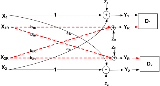
Figure 12: Equivalent model for IC-OBR Type II channel for $c_{1},c_{2}\rightarrow\infty$.

The achievable rates follow from standard arguments assuming Wyner-Ziv compression at the relay with Gaussian test channels (see, e.g., [15]). The converse for $a_{12}\geq 1,$ $a_{21}\geq 1$ follows from the results in [45]. Specifically, assume $c_{1},c_{2}\rightarrow\infty$, so that we obtain an equivalent model as shown in Fig. 12. The model in Fig. 12 is in fact equivalent to a $2\times 2$ MIMO interference channel whose channel matrices, following the notation in [45] are given by $\mathbf{H_{1}}=\left[\begin{matrix}1&0\\ 0&b_{1}\end{matrix}\right]$, $\mathbf{H_{2}}=\left[\begin{matrix}a_{21}&0\\ 0&b_{2}\end{matrix}\right]$, $\mathbf{H_{3}}=\left[\begin{matrix}a_{12}&0\\ 0&b_{1}\end{matrix}\right]$, and $\mathbf{H_{4}}=\left[\begin{matrix}1&0\\ 0&b_{2}\end{matrix}\right].$ Notice that such equivalence is due to the fact that noise correlations are immaterial in terms of the capacity region. For this channel, the assumed conditions $a_{12}\geq 1$ and $a_{21}\geq 1$ imply the strong interference regime $\mathbf{H}_{2}^{{\dagger}}\mathbf{H}_{2}\succeq\mathbf{H}_{4}^{{\dagger}}\mathbf{H}_{4}$ and $\mathbf{H}_{3}^{{\dagger}}\mathbf{H}_{3}\succeq\mathbf{H}_{1}^{{\dagger}}\mathbf{H}_{1}$, so that the capacity region can be found from [45] as

$$R_{1} \leq\mathcal{C}(P_{1})+\eta_{MAC}\mathcal{C}(b_{1}^{2}P_{1R})$$ (123a)

$$R_{2} \leq\mathcal{C}(P_{2})+\eta_{MAC}\mathcal{C}(b_{2}^{2}P_{2R})$$ (123b)

$$R_{1}+R_{2} \leq\mathcal{C}(P_{1}+a_{21}^{2}P_{2})+\eta_{MAC}\mathcal{C}(b_{1}^{2}P_{1R}+b_{2}^{2}P_{2R})$$ (123c)

$$R_{1}+R_{2} \leq\mathcal{C}(a_{12}^{2}P_{1}+P_{2})+\eta_{MAC}\mathcal{C}(b_{1}^{2}P_{1R}+b_{2}^{2}P_{2R}).$$ (123d)

This proves the desired result.

References

• [1] C. E. Shannon, “Two-way communication channels”, in Proc. Fourth Berkeley Symp. on Math. Statist. and Prob., Berkeley, California, June 1960.
• [2] R. Ahlswede, “Multi-way communication channels,” in Proc. IEEE International Symposium on Information Theory, Tsahkadsor, Armenian S.S.R., Sept. 1971.
• [3] A. Carleial, “Interference channels”, IEEE Trans. Inform. Theory, vol. 24, no. 1, pp. 60-70, Jan. 1978.
• [4] T. Cover and A. E. El Gamal, “Capacity theorems for the relay channel”, IEEE Trans. Inf. Theory, vol. 25, no. 5, pp. 572- 584, Sep. 1979.
• [5] T. Cover, A. El Gamal and M. Salehi, “Multiple access channels with arbitrarily correlated sources”, IEEE Trans. Inform. Theory, vol. 26, no. 6, pp. 648-657, Nov. 1980.
• [6] T. Han and K. Kobayashi, “A new achievable rate region for the interference channel,” IEEE Trans. Inform. Theory, vol. 27, no. 1, pp. 49-60, Jan. 1981.
• [7] H. Sato, “The capacity of the Gaussian interference channel under strong interference,” IEEE Trans. Inform. Theory, vol. 27, no. 6, pp. 786-788, Nov. 1981.
• [8] Y. Weng and D. Tuninetti, “On Gaussian interference channels with mixed interference,” in Proc. IEEE International Symposium on Information Theory (ISIT 2008), Toronto, CA, July 2008.
• [9] M. H. M. Costa, “On the Gaussian interference channel,” IEEE Trans. Inform. Theory, vol. 31, no. 5, pp. 607-615, Sep. 1985.
• [10] T. Cover and J. Thomas, Elements of Information Theory, New York: Wiley, 1991.
• [11] B. Bhargava, X. Wu, Y. Lu and W. Wang, “Integrating heterogeneous wireless technologies: a cellular aided mobile ad hoc network (CAMA)”, Journal on Mobile Networks and Applications, vol. 9, no. 4, pp. 393-408, Aug. 2004.
• [12] T. Liu and P. Viswanath, “An extremal inequality motivated by multi terminal information theoretic problems,”, IEEE Trans. Inform. Theory, vol. 53, no. 5, pp. 1839-1851, May 2007.
• [13] B. Nazer and M. Gastpar, “The case for structured random codes in network communication theorems”, in Proc. IEEE Information Theory Workshop, Lake Tahoe, California, Sept. 2007.
• [14] O. Sahin and E. Erkip, “On achievable rates for interference relay channel with interference cancellation,” in Proc. 41st Annual Asilomar Conference on Signals, Systems, and Computers, Pacific Grove, CA, Nov. 2007.
• [15] G. Kramer, Topics in Multi-User Information Theory, Foundations and Trends in Communications and Information Theory, vol. 4, no. 4-5, pp. 265-444, 2007.
• [16] O. Sahin and E. Erkip, “Achievable rates for the Gaussian interference relay channel,” in Proc. IEEE Global Telecommunications Conference, Washington, DC, Nov. 2007.
• [17] H. Chong, M. Motani, H. Garg and H. El Gamal, “On the Han-Kobayashi region for the interference channel”, IEEE Trans. on Inform. Theory, vol. 54, no. 7, July 2008.
• [18] I. Maric, R. Dabora and A. Goldsmith, “On the capacity of the interference channel with a relay,” in Proc. IEEE International Symposium on Information Theory, Toronto, Canada, July 2008.
• [19] R. Dabora, I. Maric and A. Goldsmith, “Relay strategies for interference-forwarding”, in Proc. IEEE Information Theory Workshop, Porto, Portugal, May 2008.
• [20] O. Sahin and E. Erkip, “Cognitive relaying with one-sided interference”, in Proc. Proc. 42nd Annual Asilomar Conference on Signals, Systems, and Computers, Pacific Grove, CA, Nov. 2008.
• [21] W. Yu and L. Zhou, “Gaussian Z-interference channel with a relay link: achievability region and asymptotic sum capacity,” submitted to IEEE Trans. on Inform. Theory.
• [22] S. Sridharan, S. Vishwanath, S.A. Jafar and S. Shamai, “On the capacity of cognitive relay assisted Gaussian interference channel”  in Proc. IEEE International Symposium on Information Theory, Toronto, Canada, July 2008.
• [23] O. Sahin, E. Erkip and O. Simeone, “Interference channel with a relay: models, relaying strategies, bounds”, in Proc. Information Theory and Applications Workshop, UCSD, California, Feb. 2009.
• [24] O. Sahin, O. Simeone and E. Erkip, “Interference channel aided by an infrastructure relay, ” in Proc. IEEE International Symposium on Information Theory, Seoul, Korea, June 2009.
• [25] D. Gunduz, O. Simeone, A. Goldsmith, H.V. Poor and S. Shamai, “Multiple multicasts with the help of a relay”, submitted to IEEE Trans. Inform. Theory, also available on arxiv.org [arXiv:0902.3178v1].
• [26] P. Razaghi and W. Yu, “Universal relaying for the interference channel,” in Proc. ITA Workshop, La Jolla, CA, 2010.
• [27] S. H. Lim, Y.-H. Kim, A. El Gamal and S.-Y. Chung, “Noisy network coding,” arXiv:1002.3188.
• [28] M. P. Wilson, K. Narayanan, H. Pfister and A. Sprintson, “Joint physical layer coding and network coding for bi-directional relaying”, submitted to IEEE Trans. Inform. Theory, also available on arxiv.org [arXiv:0805.0012v2].
• [29] W. Nam, S.Y. Chung and Y.H. Lee, “Capacity bounds for two-way relay channel”, in Proc. Int’l Zurich Seminar on Communications, Zurich, Switzerland, March 2008.
• [30] T.M. Cover and Y.H.Kim, “Capacity of a class of deterministic relay channels”, in Proc. IEEE International Symposium on Information Theory, Nice, France, June 2007.
• [31] A. Sanderovich, S. Shamai, Y. Steinberg and G. Kramer, “Communication via decentralized processing”, IEEE Trans. Inform. Theory, vol. 54, no. 7, pp. 3008-3023 , July 2008.
• [32] R.H. Etkin, D. N. C. Tse and H. Wang, “Gaussian interference channel capacity to within one bit”, IEEE Trans. Inform. Theory, vol. 54, no. 12, pp. 5534-5562, Dec. 2008.
• [33] V.R. Cadambe and S.A. Jafar, “Interference alignment and degrees of freedom of the $K$-user interference channel”, IEEE Trans. Inform. Theory, vol. 54, no. 8, pp. 3425-3441, Aug. 2009.
• [34] X. Shang, G. Kramer and B. Chen, “A new outer bound and noisy-interference sum-rate capacity for the Gaussian interference channels,” IEEE Trans. Inform. Theory, vol. 55, no. 2, pp. 689-699, Feb. 2009.
• [35] S. Annapureddy and V. Veeravalli, “Sum capacity of the Gaussian interference channel in the low interference regime,” in Proc. Information Theory and Applications Workshop, UCSD, California, Feb. 2008.
• [36] A. S. Motahari and A. K. Khandani, “Capacity bounds for the Gaussian interference channel”, IEEE Trans. Inform. Theory, vol. 55, no. 2, pp. 620-643, Feb. 2009.
• [37] M. Abouelseoud and A. Nosratinia, “The gateway channel: Outage analysis,” in Proc. IEEE Global Telecommunications Conference, New Orleans, LA, Dec. 2008.
• [38] D. Gündüz, A. Yener, A. Goldsmith and H. V. Poor, “Multi-way relay channel”, in Proc. IEEE International Symposium on Information Theory, Seoul, South Korea, June 2009.
• [39] H. Ghozlan, Y. Mohasseb, H. E. Gamal and G. Kramer, “The MIMO wireless switch: Relaying can increase the multiplexing gain”, in Proc. IEEE International Symposium on Information Theory, Seoul, South Korea, June 2009.
• [40] Y. Tian and A. Yener, “The Gaussian interference relay channel with a potent relay”, in Proc. IEEE Global Telecommunications Conference, Honolulu, Hawaii, Dec. 2009.
• [41] V. R. Cadambe and S. A. Jafar, “Parallel Gaussian interference channels are not always separable”, IEEE Trans. on Inform. Theory, vol. 55, No. 9, pp. 3983-3990, Sep. 2009.
• [42] L. Sankar, X. Shang, E. Erkip and H. V. Poor, “Ergodic fading interference channels: sum-capacity and separability”, submitted to IEEE Trans. on Inform. Theory, June 2009, also available on arxiv.org [arXiv:0906.0744v1].
• [43] X. Shang, B. Chen, G. Kramer and H.V. Poor, “Noisy-interference sum-rate capacity of parallel Gaussian interference channels”, submitted to IEEE Trans. on Inform. Theory, March 2009, also available on arxiv.org [arXiv:0903.0595v1].
• [44] S. W. Choi and S. Chung, “On the separability of parallel Gaussian interference channels”, in Proc. IEEE International Symposium on Information Theory, Seoul, South Korea, June 2009.
• [45] X. Shang, B. Chen, G. Kramer and H. V. Poor, “Capacity regions and sum-rate capacities of vector Gaussian interference channels”, submitted to IEEE Trans. on Inform. Theory, July 2009, also available on arxiv.org [arXiv:0907.0472v1].