Effect of spatial inhomogeneity on the mapping between strongly interacting fermions and weakly interacting spins

Abstract

A combined analytical and numerical study is performed of the mapping between strongly interacting fermions and weakly interacting spins, in the framework of the Hubbard, t-J and Heisenberg models. While for spatially homogeneous models in the thermodynamic limit the mapping is thoroughly understood, we here focus on aspects that become relevant in spatially inhomogeneous situations, such as the effect of boundaries, impurities, superlattices and interfaces. We consider parameter regimes that are relevant for traditional applications of these models, such as electrons in cuprates and manganites, and for more recent applications to atoms in optical lattices. The rate of the mapping as a function of the interaction strength is determined from the Bethe-Ansatz for infinite systems and from numerical diagonalization for finite systems. We show analytically that if translational symmetry is broken through the presence of impurities, the mapping persists and is, in a certain sense, as local as possible, provided the spin-spin interaction between two sites of the Heisenberg model is calculated from the harmonic mean of the onsite Coulomb interaction on adjacent sites of the Hubbard model. Numerical calculations corroborate these findings also in interfaces and superlattices, where analytical calculations are more complicated.

I Introduction

Strongly interacting fermions are part of some of todays most studied physical systems. In cuprate and manganite systems, for example, strongly correlated electrons are held responsible for high-temperature superconductivity and colossal magnetoresistance, respectively.electrons1 ; electrons2 ; electrons3 Systems of strongly interacting fermionic atoms can be realized in optical lattices, and are currently under intense investigation due to the possibility to use them as quantum simulators for understanding phenomena of condensed matter physics.atoms1 ; atoms2 ; atoms3

Since the seminal works of Wigner on the low-density electron crystalwigner and of Mott on the metal-insulator transitionmott it is known that strong repulsive particle-particle interactions suppress itineracy and favor localization.mit In the localized state, the repulsive interaction is minimized, and charge degrees of freedom are frozen out. The dominating interactions in this state are magnetic.

Mathematically, strongly interacting fermions are frequently described by the Hubbard model, which in one dimension is defined by the Hamiltonian

$$\hat{H}^{Hubb}=-t\sum_{i\sigma}(\hat{c}_{i\sigma}^{\dagger}\hat{c}_{i+1,\sigma}+H.c.)+U\sum_{i}\hat{n}_{i\uparrow}\hat{n}_{i\downarrow},$$ (1)

where $\hat{c}_{i\sigma}^{\dagger}$ and $\hat{c}_{i\sigma}$ are fermionic creation and destruction operators, $\hat{n}_{i\sigma}=\hat{c}_{i\sigma}^{\dagger}\hat{c}_{i\sigma}$ is the particle-density operator, $U$ the onsite interaction and $t$ the hopping parameter.

For sufficiently strong interactions, the Hubbard model can be expanded in powers of $t/U$. (Below we quantify what interactions can be considered ‘sufficiently strong’.) The leading term of this expansion is the t-J model,

$$\hat{H}^{tJ} = -t\sum_{i\sigma}(\hat{c}_{i\sigma}^{\dagger}\hat{c}_{i+1,\sigma}+H.c.)$$ (2)

$$+\frac{4t^{2}}{U}\sum_{i}\left[\vec{\hat{S}}_{i}\cdot\vec{\hat{S}}_{i+1}-\frac{\hat{n}_{i}\hat{n}_{i+1}}{4}\right],$$

where $\vec{\hat{S}}_{i}$ is the spin one-half vector operator at each site. This model is frequently taken to be the starting point in investigations of doped cuprates.

For a half-filled system, in which the number of fermions $N$ equals the number of lattice sites $L$, the average density $n=N/L$ is unity. Since there are no empty sites, hopping is suppressed, and the t-J model reduces to the antiferromagnetic Heisenberg model

$$\hat{H}^{Heis}=J\sum_{i}\left[\vec{\hat{S}}_{i}\cdot\vec{\hat{S}}_{i+1}-\frac{1}{4}\right],$$ (3)

where $J=4t^{2}/U$ and charge fluctuations are completely frozen out. The original system of strongly interacting itinerant fermions ($U/t\gg 1$) has thus been mapped on a system of localized spins with weak antiferromagnetic interactions ($0\leq J/t\ll 1$).

The mathematics and the physics of this mapping are very well understood and discussed in the textbook literature.auerbach ; fulde The mapping of strongly interacting itinerant fermions on weakly interacting localized spins is a standard concept of condensed-matter physics, routinely used in the interpretation of experiments on strongly correlated solids. Recently, however, three important classes of systems have been discovered or created that call for a reconsideration and more detailed investigation of this mapping.

It is well known that many strongly correlated systems are characterized by nanoscale spatial inhomogeneity. Such inhomogeneity can take the form of irregular spatial variations of system properties, such as observed by scanning-tunneling microscope techniques in many cuprates and similar materials,electrons2 ; inhom0 ; inhom1 ; inhom2 ; inhom3 ; inhom4 or the form of regular spatial variations such as in naturally occurring or man-made superlattice structures.paiva ; malvezzi ; malvezzi2 ; superl3 ; superl4 In the presence of either type of inhomogeneity, the parameters characterizing the model Hamiltonian become site dependent. In the simplest case, with which we are mostly concerned here, the above homogeneous Hubbard model is replaced by an inhomogeneous model of the form

$$\hat{H}^{Hubb}_{inh}=-t\sum_{i\sigma}(\hat{c}_{i\sigma}^{\dagger}\hat{c}_{i+1,\sigma}+H.c.)+\sum_{i}U_{i}\hat{n}_{i\uparrow}\hat{n}_{i\downarrow},$$ (4)

in which the onsite interaction $U_{i}$ varies from site to site.

A second class of systems we are concerned with here are nanoscale devices. In the modeling of such devices inhomogeneities in the model parameters occur simply because on the nanoscale the effect of the surface can no longer be neglected, and also because a typical device combines more than one material, with the resulting interface automatically implying the existence of spatial variations in the system parameters.

Finally, in still another line of research, ultracold atom gases have been trapped optically and arranged in optical lattices.atoms1 ; atoms2 In optical traps the system parameters can be controlled and varied in ways not possible in solid-state situations. In particular, the onsite interaction $U_{i}$ can attain values $U/t\approx 100$ or larger. Such values are way beyond what is considered ‘strongly correlated’ in solid-state physics.

Motivated by all these systems, we present, in the present paper, a combined analytical and numerical study of the mapping from the Hubbard model to the Heisenberg model in the presence of spatial inhomogeneity. In Sec. II we investigate the rate of the mapping, as measured by the difference in ground-state energies of the Hamiltonians. We allow the interaction strength to go beyond its typical solid-state values and to enter the ultrastrong regime attainable for cold atoms.

In Sec. III we turn to our main subject, the inhomogeneous Hubbard model of Eq. (4). In Sec. III.1 we investigate analytically the case of a single impurity, described as one site with a value of $U$ differing from all others, and show that the Hubbard-to-Heisenberg mapping is preserved essentially in its homogeneous form, provided the effective $J$ is calculated from the harmonic mean of the values of $U$ on the sites connected by $J$. We illustrate this finding numerically, by contrasting, for an impurity system, results obtained from the harmonic mean with results obtained from the arithmetic, geometric and quadratic means. In Sec. III.2 we show that the harmonic mean allows to extend the Hubbard-to-Heisenberg mapping to systems with more complicated types of spatial inhomogeneity, such as superlattices, disordered systems and interfaces between different materials. Section IV contains our conclusions.

II Rate of the mapping for translationally invariant systems

In a first step, to provide the background for the later investigations, we consider spatially homogeneous infinite Hubbard and Heisenberg chains, and investigate the rate of the approach of the ground-state energies of both models as a function of $U$. This allows us to quantify the rate at which charge fluctuations are frozen out.

The per-site ground-state (GS) energy of the Heisenberg chain in the thermodynamic limit is

$$e^{Heis}(J)=\lim_{L\to\infty}{E^{Heis}\over L}=-J\ln(2).$$ (5)

The per-site GS energy of infinite half-filled ($n=1$) Hubbard chain at $U/t\to\infty$ is

$$e^{Hubb}(n=1,{U\over t}\to\infty)=\lim_{L\to\infty}{E^{Hubb}\over L}=-{4t^{2}\over U}\ln(2).$$ (6)

Both expressions become identical for $J=4t^{2}/U$. In order to quantitatively investigate the mapping at finite $U/t$, we calculate $e^{Hubb}(n=1,U)$ by numerically solving the Bethe-Ansatz integral equationsliebwu ; shiba as a function of $U$ and compare the result to the energy of the Heisenberg model at the corresponding value of $J$, i.e. $e^{Heis}(J=4t^{2}/U)$. The result is displayedfoot1 in Fig. 1.

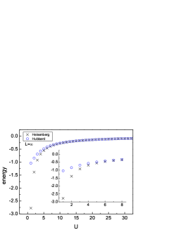
Figure 1: Per-site GS energy as a function of interaction in the thermodynamic limit. Comparison between the Heisenberg with $J=4t^{2}/U$ and the half-filled Hubbard chain. The main figure includes values of $U$ that can be realized in systems of trapped cold atoms, while the inset displays results for values of $U$ typical of weakly and strongly correlated solids.

In Table 1 we show the relative percentage deviation between the GS energies,

$$D(\%)=100\frac{e^{Hubb}-e^{Heis}}{e^{Hubb}},$$ (7)

for various representative values of $U$. This comparison between both models becomes trivial, once the Bethe-Ansatz solution is available, but already leads to a first somewhat unexpected conclusion. Frequently, the Heisenberg model is taken to be the starting point for a description of undoped antiferromagnetic insulating parent compounds of high-temperature superconductors. The effect of doping is accounted for by going from the Heisenberg to the t-J model, arguing that the latter should be a reasonable approximation to the Hubbard model for the involved large values of $U$.

What the comparison in Fig. 1 and Table 1 shows is that for values of $U$ that are representative of cuprate materials the t-J or Heisenberg models provide at best a semiquantitative approximation to the Hubbard model. At $U=6$ the difference between both ground-state energies is approximately $10\%$. Charge fluctuations are thus not yet frozen out for such $U$, even at half filling. The rather large deviation observed shows that the mapping of strongly interacting fermions onto weakly interacting spins is not quantitatively reliable for, e.g., cuprate systems at realistic values of $U$. There is no doubt, of course, that the t-J model captures the correct physics of the large-U Hubbard model – the above questioning only refers to the accuracy to which one needs to obtain a solution of the former, given that in the parameter regime typical of strongly-correlated solids it is itself only a moderately accurate representation of the latter.

Table 1: Relative percentage deviation of the per-site GS energies for values of $U$ typical of weakly correlated solids ($U=1$), strongly correlated solids ($U=6$) and values that are attainable for atoms in optical traps.

$U$	1	6	10	20	50	100	200
$D(\%)$	-166.50	-10.01	-3.78	-0.97	-0.16	-0.04	-0.01

We note that this analysis is based on GS energies. An alternative comparison between both Hamiltonians would proceed in terms of the overlap of their wave functions, instead of the difference of their energies. Our main interest in this initial investigation is to investigate for which values of $U$ the mapping breaks down, and for this it is enough to find one quantity that is not properly reproduced. Thus, if we use our analysis to indicate when the mapping does not hold, we are on the safe side by using energies. Still another, and indeed more fundamental, mode of analysis proceeds by directly comparing the Hamiltonians. We use this procedure in Sec. III.1, where our interest is not only in when the mapping breaks down, but also in how it can be restored.

III Mapping in the presence of spatial inhomogeneity

We now turn to systems where the inhomogeneity occurs not only at the surface, due to finite size, but also in the bulk. A typical case is that of a localized impurity or defect, modeled by one site with onsite interaction differing from that of all the others. We take this simple system as representative of Hubbard models with broken translational symmetry, and focus most of our analysis on it. The extension of our conclusions to interfaces and superlattices is discussed in Sec. III.2.

Intuitively, one would expect that a localized perturbation of the homogeneous Hubbard model should only produce a similarly localized perturbation of the homogeneous Heisenberg model. However, the relation between both models involves a projection on the subspace with no double occupation, together with an expansion in inverse powers of $U$,auerbach ; fulde and it is not clear from the outset to what extent these operations preserve the above naive expectation of locality.

In fact, there is one sense in which the mapping, if it continues to exist, cannot be local: $U$ is defined on one site, while $J$ connects two adjacent sites. While this difference is almost irrelevant in the homogeneous case where all sites are equivalent and translational symmetry rules, it becomes important in the inhomogeneous case, where any change in the onsite $U$ on the Hubbard model must affect the corresponding intersite $J$ for at least two sites of the Heisenberg model. This is illustrated in Fig. 2.

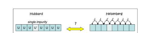
Figure 2: Illustration of the inhomogeneous Hubbard model with a single impurity $U^{\prime}\neq U$, and its putative relation to an inhomogeneous Heisenberg model with two bond defects $J^{\prime}\neq J$.

The questions to address are thus (i) whether the mapping still exists in the absence of translational symmetry, (ii) how to calculate the Heisenberg $J$ from the Hubbard $U$ in inhomogeneous systems, and (iii) if the mapping is as local as possible, i.e., involves only sites adjacent to the impurity site, or requires a higher degree of nonlocality. In next subsections we address these questions analytical and numerically.

III.1 A single impurity

We start with the one-dimensional Hubbard model in the presence of a single impurity at site $k$ with onsite interaction $U^{\prime}$ differing from the background value $U$ on all other sites $i\neq k$,

$$\hat{H}^{Hubb}_{inh} = -t\sum_{i\sigma}(\hat{c}_{i\sigma}^{\dagger}\hat{c}_{i+1,\sigma}+H.c.)+U\sum_{i\neq k}\hat{n}_{i\uparrow}\hat{n}_{i\downarrow}$$ (8)

$$+U^{\prime}\hat{n}_{k\uparrow}\hat{n}_{k\downarrow}.$$

The standard proof of the mapping from the Hubbard to the t-J modelauerbach ; fulde can be repeated for this Hamiltonian and leads to the inhomogeneous t-J model with Hamiltonian

$$\hat{H}_{inh}^{tJ} = -t\sum_{i\sigma}(\hat{c}_{i\sigma}^{\dagger}\hat{c}_{i+1,\sigma}+H.c.)\hskip 28.45274pt$$

$$+\frac{4t^{2}}{U}\sum_{i\neq k}\left[\vec{\hat{S}}_{i}\cdot\vec{\hat{S}}_{i+1}-\frac{\hat{n}_{i}\hat{n}_{i+1}}{4}\right]$$

$$+\frac{4t^{2}}{U^{\prime}}\left[\vec{\hat{S}}_{k}\cdot\vec{\hat{S}}_{k+1}-\frac{\hat{n}_{k}\hat{n}_{k+1}}{4}\right],$$

where we assumed that both $U$ and $U^{\prime}$ are much larger than $t$. We rewrite this Hamiltonian by extracting one term from the sum over $i\neq k$ to obtain

$$\hat{H}_{inh}^{tJ} = -t\sum_{i\sigma}(\hat{c}_{i\sigma}^{\dagger}\hat{c}_{i+1,\sigma}+H.c.)$$

$$+\frac{4t^{2}}{U}\sum_{i\neq k,l}\left[\vec{\hat{S}}_{i}\cdot\vec{\hat{S}}_{i+1}-\frac{\hat{n}_{i}\hat{n}_{i+1}}{4}\right]$$

$$+\frac{4t^{2}}{U}\left[\vec{\hat{S}}_{k}\cdot\vec{\hat{S}}_{k+1}-\frac{\hat{n}_{k}\hat{n}_{k+1}}{4}\right]$$

$$+\frac{4t^{2}}{U^{\prime}}\left[\vec{\hat{S}}_{l}\cdot\vec{\hat{S}}_{l+1}-\frac{\hat{n}_{l}\hat{n}_{l+1}}{4}\right].$$

Now we take the average density $n=N/L=1$. A priori this average can be obtained from many different distributions $n_{i}$. However, since we are already in the limit $U,U^{\prime}\gg t$, the total interaction energy on the background and the impurity sites is minimized by the particular distribution $n_{i}=1$ for all $i$. Deviations from this are due to hopping processes that become increasingly suppressed as $U$ and $U^{\prime}$ grow. Thus the Hamiltonian (III.1) at $n=1$ reduces to

$$\hat{H}_{inh}^{tJ}(n=1) = +\frac{4t^{2}}{U}\sum_{i\neq k,l}\left[\vec{\hat{S}}_{i}\cdot\vec{\hat{S}}_{i+1}-\frac{1}{4}\right]$$

$$+4t^{2}\left(\frac{1}{U}+\frac{1}{U^{\prime}}\right)\left[\vec{\hat{S}}_{l}\cdot\vec{\hat{S}}_{l+1}-\frac{1}{4}\right],$$

where we chose $l$ as a neighbor site of $k$, $k=l+1$, such that $\vec{\hat{S}}_{l}\cdot\vec{\hat{S}}_{l+1}=\vec{\hat{S}}_{k}\cdot\vec{\hat{S}}_{k+1}$. This, in turn, can be written as

$$H^{Heis}_{inh}=J\sum_{i\neq l,l+1}\left[\vec{\hat{S}}_{i}\cdot\vec{\hat{S}}_{i+1}-\frac{1}{4}\right]+2J^{\prime}\left[\vec{\hat{S}}_{l}\cdot\vec{\hat{S}}_{l+1}-\frac{1}{4}\right],$$

(12)

which has the form of a spatially inhomogeneous Heisenberg model with background interaction $J=4t^{2}/U$ and two bond defects $J^{\prime}=4t^{2}/\bar{U}^{H}$, where $\bar{U}^{H}$ is the harmonic mean of $U$ and $U^{\prime}$,

$$\bar{U}^{H}=\frac{2UU^{\prime}}{U+U^{\prime}}.$$ (13)

This derivation tells us that the Hubbard model with a single impurity can indeed be mapped onto a Heisenberg model with two bond defects, provided the impurity site and the background sites both have repulsive interactions that are much larger than $t$, and that the $J$ connecting the impurity site with its neighbors to the left and to the right is calculated from the harmonic mean of the two onsite interactions. The mapping then still exists and is seen to be as local as possible, in the sense explained above.

In order to investigate the rate of the mapping in inhomogeneous systems, we now perform a numerical investigation of both models. For illustration we also include in these calculations the quadratic, arithmetic and geometric means,

$$\bar{U}^{Q} = \sqrt{\frac{U^{2}+U^{\prime 2}}{2}}$$ (14)

$$\bar{U}^{A} = \frac{U+U^{\prime}}{2}$$ (15)

$$\bar{U}^{G} = \sqrt{UU^{\prime}}.$$ (16)

Both the inhomogeneous Hubbard model with $n=1$ and one $U^{\prime}\neq U$ and the inhomogeneous Heisenberg model with two $J^{\prime}\neq J$ are diagonalized numerically, and compared by means of the deviation between their GS energies. We use the same method of analysis as in Sec. II, this time, however, applied to impurity systems.

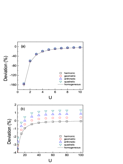
Figure 3: Relative percentage deviation between the GS energies of the single-impurity Hubbard chain and the two-defect Heisenberg chain, obtained from numerical diagonalization, adopting $J^{\prime}=J(\bar{U})$ with four different choices for the average $\bar{U}$: (a) values of $U$ that are typical of solids and (b) values of $U$ that are attainable in systems of optically trapped atoms. System parameters: $L=8$ sites, $N=8$ fermions, open boundary conditions, impurity strength $U^{\prime}=3U/2$.

Our key result is contained in Fig. 3, which displays the relative percentage deviation between the inhomogeneous Hubbard and the inhomogeneous Heisenberg models with $J^{\prime}=J(\bar{U})$ for each of the four averages. The solid line represents the corresponding deviation obtained for the impurity-free Hubbard and Heisenberg models, where $U$ and $J=4t^{2}/U$ are the same across the system.

Figure 3–(a) demonstrates clearly that if the background $U$ is so small that the mapping is not quantitatively reliable even in the homogeneous system (this includes the values found in cuprates), then it is also not reliable in inhomogeneous systems, regardless of the choice made for relating the bond defect to the impurity size. On the other hand, Fig. 3–(b) makes a different statement: once the background $U$ is large enough to permit the basic Hubbard-to-Heisenberg mapping to function, all four averages lead to values of $J^{\prime}=4t^{2}/\bar{U}$ that are equal (H) or different (A,G,Q) than obtained in the homogeneous system.

This is unequivocal numerical evidence that the mapping of strongly interacting fermions on weakly interacting spins survives in the presence of impurities and defects. In order to probe the locality of the mapping we have also performed numerical experiments with averages over more than two neighboring sites, calculating $J^{\prime}(\bar{U})$ from, e.g. a weighted average of the interactions at the sites connected by $U$ and their nearest-neighbor sites. No improvement (and frequently even worse results) with regard to the simple two-site averages was obtained, indicating that the mapping is indeed local.

At first sight more surprising is that the alternative averaging procedures produce even smaller deviations for some values of $U$, Fig. 3–(b). However, for still larger values of $U$ and $U^{\prime}$ (where the mapping should as a matter of principle get better and better) all these alternative averages produce deviations that continue to grow and yield $D>0$, while the harmonic mean correctly approaches the limit $D=0$ as $U,U^{\prime}\to\infty$. This shows that only the harmonic mean has a chance to correctly describe the fermion-to-spins mapping in inhomogeneous systems, while the lower deviations of the other averages for some parameter regimes only occur because the curves are monotonous so that there is always a range of values for which they are close to zero.

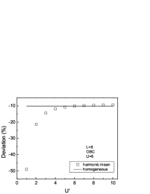
Figure 4: Deviation of GS energies of the half-filled Hubbard model and the corresponding Heisenberg model as a function of impurity strength, obtained from the harmonic mean. At $U^{\prime}=U=6$ the system is homogeneous (except for the presence of the boundary) and the deviation is the same obtained in Sec. II.

We note that in Fig. 3 the ratio of $U$ and $U^{\prime}$ was held fixed, such as to guarantee that for all values of $U$, $U^{\prime}$ was always substantially different from $U$ ($U^{\prime}=3U/2$). In Fig. 4 we present the complementary analysis in which the background $U$ is held fixed and the impurity interaction is varied from $U^{\prime}<U$ to $U^{\prime}>U$. For this comparison we consistently adopted the harmonic mean. A first feature that jumps to the eye is that a single site with $U^{\prime}<U$ is enough to substantially deteriorate the mapping. By contrast, a single site with $U^{\prime}>U$ leads only to a slight reduction of the deviation between GS energies, much less than the deterioration observed for $U^{\prime}<U$.

This behavior arises from the hopping terms. Both at $U^{\prime}>U$ (more repulsive impurity site) and at $U^{\prime}<U$ (less repulsive site) the on-site density at the impurity site slightly deviates from that at the background sites, as long as $U$ and $U^{\prime}$ are both finite. In the latter case, however, hopping processes involving the impurity site increase as $U^{\prime}$ is reduced, and the Hubbard-to-Heisenberg mapping becomes correspondingly worse, while in the former case hopping continues to be strongly suppressed. The behavior displayed by Fig. 4 is thus consistent with what one would expect on the basis of the derivation leading from Eq.(8) to Eq.(12).

Independently of, but in agreement with, our previous analytical derivation we thus find that the harmonic mean solves the problem exactly for a single impurity and for sufficiently large interactions, while the other possible averages do not. However there is still one question concerning this result and it is addressed in next section: is the harmonic mean able to recover the mapping in more complex inhomogeneities?

III.2 More complex inhomogeneities

In view of our initial discussion of naturally occurring or man-made inhomogeneity in strongly correlated systems, it becomes important to extend our analysis to more complex inhomogeneities than boundaries or single impurities. We here briefly describe our findings on three of these: interfaces, superlattices and disordered systems.

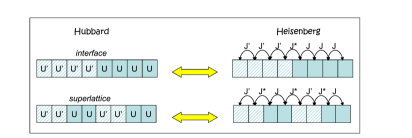
Figure 5: Illustration of simple interface and superlattice structures in the Hubbard model, and their counterparts in the Heisenberg model.

Interfaces and superlattices can be described in the Hubbard and Heisenberg models as shown schematically in Fig. 5. While the description of superlattices by means of periodic spatial variations of $U$ is the standard choice,paiva which we here also adopt, it has been pointed out that a periodic modulation of local electric potentials can bring about a much larger change in the system properties.malvezzi ; malvezzi2 ; fc2008 Here, however, we are interested in the Hubbard-to-Heisenberg transition, which is driven by the interaction and not by local potentials, and therefore we follow the usual prescription to ignore possible local electric fields in the superlattice structure.

We note that in the superlattice and the interface geometry we now have three different spin-spin interactions, one, $J$, being calculated from $U$, another, $J^{\prime}$, from $U^{\prime}$ and the last, $J^{*}$, from $U$ and $U^{\prime}$, as indicated in Fig. 5. Figure 6 shows that for large $U$ and $U^{\prime}$ the GS energies of the Heisenberg model, when calculated from the harmonic mean, become identical to those of the corresponding Hubbard model, for all investigated geometries. In this sense, the mapping continues to work and to be as local as possible. Note that this would not be true for the arithmetic, geometric and quadratic means, whose deviations increase for large $U$ and $U^{\prime}$.

The fact that the Hubbard-Heisenberg deviation for the superlattice is larger than that for the interface can be understood on purely geometric grounds, as a consequence of the locality of the mapping and the nature of the harmonic mean: By comparing the distribution of $J$ values, Fig. 5, we see that in going from the interface to the superlattice the number of interactions $J$ and $J^{\prime}$ is reduced by the same amount, while that of interactions $J^{*}$ increases. Since $J^{\prime}<J^{*}<J$, a reduction of the number of sites with $J^{\prime}$ worsens the mapping while a reduction of the number of sites with $J$ improves it. To see what the net effect is we must take into account the interaction $J^{*}$, which replaces $J$ and $J^{\prime}$. This interaction is calculated from $\bar{U}$, the harmonic mean of $U$ and $U^{\prime}$. The harmonic mean of any two positive numbers is less or equal their arithmetic mean, so that $\bar{U}$ is closer to $U$ than to $U^{\prime}$ and $J^{*}$ is closer to $J$ than to $J^{\prime}$. The substitution of an equal number of $J$ and $J^{\prime}$ by $J^{*}$ thus has the effect of effectively increasing the number of ‘bad’ sites, and therefore to deteriorate the quality of the mapping. This is what the data show: the deviation for the superlattice is larger than that for the interfaces, if all other parameters are chosen the same.

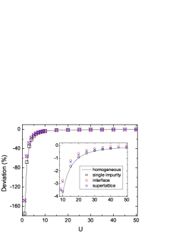
Figure 6: Relative percentage deviation between the GS energies of the Hubbard and the Heisenberg model for a superlattice structure, an interface, a single-impurity system and a system that is spatially homogeneous (except for the surface). In the superlattice and the interface system the number of sites with $U$ and $U^{\prime}$ is the same, respectively, the only difference being in their geometric distribution. System parameters: $L=8$, $U^{\prime}=3U/2$, $J^{\prime}=4t^{2}/U^{\prime}$ and $J^{*}=4t^{2}/\bar{U}$, where $\bar{U}$ is calculated from the harmonic mean of $U$ and $U^{\prime}$.

This analysis shows that the harmonic-mean prescription continues to be usable for these more complex geometries and that the effect of the geometrical distribution of $U$ and $U^{\prime}$ sites across the system can be understood and analyzed essentially on a site-by-site basis. This is a direct consequence of the locality of the mapping.

Disordered systems can be modeled simply by considering a random distribution of impurities instead of just one. While a complete analysis of disordered systems requires statistical analysis of data resulting from a large number of realizations of the disorder, an analysis of a few representative cases is enough to conclude that the single-impurity results are not changed, in their essence, when the impurity concentration is increased.

Specifically, we find that if all impurities have $U^{\prime}>U$ a higher concentration of impurities reduces the deviation between the GS energies. Keeping the concentration fixed and increasing $U^{\prime}/U$ also reduces the deviation, but to a much smaller degree. On the other hand, if all impurities have $U^{\prime}<U$ the agreement is naturally worsened. However, in the $U^{\prime}<U$ case the decisive factor is not so much the concentration of impurities but their strength, as measured by $U^{\prime}/U$. This inversion in the effect of concentration and strength of the impurities can be understood on the basis of Fig. 4, which shows that for a single impurity with $U^{\prime}<U$ the deviation rapidly increases as $U^{\prime}$ becomes more different from $U$, while for $U^{\prime}>U$ it decreases only very slowly and almost saturates as the impurity sites effectively drop out of the system.

This discussion shows that it is possible to control the degree of the fermion-spin mapping by means of the introduction of a suitable concentration of impurities of suitable strength. This possibility may be useful in the design of nanoscale devices based on strongly correlated systems, whose properties can be tailored from electron-like to spin-like by introducing suitable disorder. We note in passing that this is a strong-interaction effect, completely different from the itinerant-to-localized transition resulting from disorder in Anderson localization.

IV Conclusions

In the homogeneous situation, in which all sites are equivalent, the mapping is characterized by the behavior of the system as a function of the onsite interaction $U$. Not unexpectedly, the Heisenberg model is found to be a good approximation to the t-J and the Hubbard model at $n=1$. Somewhat more unexpected is that the Heisenberg model is rather a bad approximation to the Hubbard model at $n=1$ even for values of $U$ that are considered strongly correlated in solid-state applications. Only at $U$ near 20 has the deviation dropped to about one percent. The standard mapping thus only becomes quantitatively reliable for values of $U$ that are hard to reach in the solid state, but have already been demonstrated in cold-atom systems.

In inhomogeneous situations, translational symmetry is broken. An analytical calculation for the simple case of a single impurity suggests that the mapping can be preserved in terms of the harmonic mean. Moreover, in terms of this mean the mapping is as local as possible, i.e., the value of the Heisenberg $J$ between two sites is only determined from the value of the Hubbard $U$ at these two sites. Numerical calculations illustrate and corroborate this finding. This is more than a mathematical, or numerical, result: it means that the physics of the mapping, i.e., the gradual freezing out of the charge-degrees of freedom and the localization arising from the concomitant suppression of double occupation, is essentially the same regardless of the geometry and the presence or absence of translational symmetry.

The harmonic-mean prescription can be used easily and reliably for a wide variety of spatial inhomogeneities. Once the basic mapping is understood, the harmonic-mean prescription allows one to interpret and even to predict the behavior of much more complicated systems, without going through detailed analytical or computationally expensive numerical calculations.

Acknowledgments This work was supported by Brazilian funding agencies FAPESP and CNPq. We thank Vivaldo Campo Jr. for providing us with his exact diagonalization code for the Hubbard model, and Fabiano C. Souza and Valter L. Líbero for providing us with their exact diagonalization code for the Heisenberg model.

References

- (1) E. Dagotto, Rev. Mod. Phys. 66, 763 (1994).
- (2) M. B. Salamon and M. Jaime, Rev. Mod. Phys. 73, 583 (2001).
- (3) J. Quintanilla and C. Hooley, Physics World 22, 32 (2009).
- (4) J. I. Cirac and P. Zoller, Science 301, 176 (2003).
- (5) I. Bloch, J. Dalibard, and W. Zwerger, Rev. Mod. Phys. 80, 885 (2008).
- (6) S. Giorgini, L. P. Pitaevskii and S. Stringari, Rev. Mod. Phys. 80, 1215 (2008).
- (7) E. P. Wigner, Phys. Rev. 46, 1002 (1934).
- (8) N. Mott, Metal-Insulator Transitions, Taylor & Francis, New York, (1974)
- (9) M. Imada, A. Fujimori, and Y. Tokura, Rev. Mod. Phys. 70, 1039 (1998).
- (10) A. Auerbach, Interacting Electrons and Quantum Magnetism, Springer, New York (1994).
- (11) P. Fulde, Electron Correlations in Molecules and Solids, Springer, Heidelberg (1995).
- (12) E. Dagotto, Science 309, 257 (2005).
- (13) A. R. Bishop, S. R. Shenoy, and S. Sridhar, Intrinsic Multiscale Structure and Dynamics in Complex Electronic Oxides, World Scientific, New Jersey (2003).
- (14) K. M. Lang, V. Madhavan, J. E. Hoffman, E. W. Hudson, H. Eisaki, S. Uchida, and J. C. Davis, Nature 415, 412 (2002).
- (15) S. H. Pan, J. P. O’Neal, R. L. Badzey, C. Chamon, H. Ding, J. R. Engelbrecht, Z. Wang, H. E. Eisaki, S. Uchida, A. K. Gupta, K.-W. Ng, E. W. Hudson, K. M. Lang, and J. C. Davies, Nature 413, 282 (2001).
- (16) D. J. Derro, E. W. Hudson, K. M. Lang, S. H. Pan, J. C. Davis, J. T. Markert, and A. L. de Lozanne, Phys. Rev. Lett. 88, 097002 (2002).
- (17) T. Paiva and R. R. dos Santos, Phys. Rev. B 65, 153101 (2002); ibid 62, 7007 (2000); 58, 9607 (1998); Phys. Rev. Lett. 76, 1126 (1996).
- (18) M. F. Silva, N. A. Lima, A. L. Malvezzi and K. Capelle, Phys. Rev. B 71, 125130 (2005).
- (19) N. A. Lima, A. L. Malvezzi and K. Capelle, Sol. State Com. 144, 557 (2007).
- (20) D. Góra, K. J. Rościszewski, and A. M. Oleś, J. Phys.: Condens. Matter 10, 4755 (1998).
- (21) M. Noh, D. C. Johnson, and G. S. Elliott, Chem. Mater. 1̱2, 2894 (2000).
- (22) E. H. Lieb, F. Y. Wu, Phys. Rev. Lett. 20, 1445 (1968).
- (23) H. Shiba, Phys. Rev. B 6, 930 (1972).
- (24) In all figures and tables we take , i.e., measure energies in multiples of the hopping parameter.
- (25) V. V. França and K. Capelle, Phys. Rev. Lett. 100, 070403 (2008).
- (26) R. Jördens, N. Strohmaier, K. Günter, H. Moritz and T. Esslinger, Nature 455, 204 (2008).