Filtrage vaste marge pour l’étiquetage séquentiel à noyaux de signaux

Résumé

Ce papier traite de l’étiquetage séquentiel de signaux, c’est-à-dire de discrimination pour des échantillons temporels. Dans ce contexte, nous proposons une méthode d’apprentissage pour un filtrage vaste-marge séparant au mieux les classes. Nous apprenons ainsi de manière jointe un SVM sur des échantillons et un filtrage temporel de ces échantillons. Cette méthode permet l’étiquetage en ligne d’échantillons temporels. Un décodage de séquence hors ligne optimal utilisant l’algorithme de Viterbi est également proposé. Nous introduisons différents termes de régularisation, permettant de pondérer ou de sélectionner les canaux automatiquement au sens du critère vaste-marge. Finalement, notre approche est testée sur un exemple jouet de signaux non-linéaires ainsi que sur des données réelles d’Interface Cerveau-Machine. Ces expériences montrent l’intérêt de l’apprentissage supervisé d’un filtrage temporel pour l’étiquetage de séquence.

SVM, Étiquetage séquentiel, Filtrage

1 Introduction

Signal sequence labeling is a classical machine learning problem that typically arises in Automatic Speech Recognition (ASR) or Brain Computer Interfaces (BCI). The idea is to assign a label for every sample of a signal while taking into account the sequentiality of the samples. For instance, in speaker diarization, the aim is to recognize which speaker is talking along time. Another example is the recognition of mental states from Electro-Encephalographic (EEG) signals. This mental states are then mapped into commands for a computer (virtual keyboard, mouse) or a mobile robot, hence the need for sample labeling Blankertz et al., (2004); Millán, (2004).

One widely used approach for performing sequence labeling is Hidden Markov Models (HMMs), cf. (Cappé et al., , 2005). HMMs are probabilistic models that may be used for sequence decoding of discrete states observations. In the case of continuous observations such as signal samples or vectorial features extracted from the signal, Continuous Density HMMs are considered. When using HMM for sequence decoding, one needs to have the conditional probability of the observations per hidden states (classes), which is usually obtained through Gaussian Mixtures (GM) (Cappé et al., , 2005). But this kind of model performs poorly in high dimensional spaces in terms of discrimination, and recent works have shown that the decoding accuracy may be improved by using discriminative models (Sloin & Burshtein, , 2008). One simple approach for using discriminative classifiers in the HMM framework has been proposed by Ganapathiraju et al., (2004). It consists in learning SVM classifiers known for their better robustness in high dimension and to transform their outputs to probabilities using Platt’s method (Lin et al., , 2007), leading to better performances after Viterbi decoding. However, this approach supposes that the complete sequence of observation is available, which corresponds to an offline decoding. In the case of BCI application, a real time decision is often needed (Blankertz et al., , 2004; Millán, , 2004), which restricts the use of the Viterbi decoding.

Another limit of HMM is that they cannot take into account a time-lag between the labels and the discriminative features. Indeed, in this case some of the learning observations are mislabeled, leading to a biased density estimation per class. This is a problem in BCI applications where the interesting information are not always synchronized with the labels. For instance, Pistohl et al., (2008) showed the need of applying delays to the signal, since the neuronal activity precedes the actual movement. Note that they selected the delay through validation. Another illustration of the need of time-lag automated handling is the following. Suppose we want to interact with a computer using multi-modal acquisitions (EEG,EMG,…). Then, since each modality has its own time-lag with respect to neural activity as shown by Salenius et al., (1996), it may be difficult to manually synchronize all modalities and better adaptation can be obtained by learning the “best” time-lag to apply to each modality channel.

Furthermore, instead of using a fixed filter as a preprocessing stage for signal denoising, learning the filter may help in adapting to noise characteristics of each channel in addition to the time-lag adjustment. In such a context, Flamary et al., (2010) proposed a method to learn a large margin filtering for linear SVM classification of samples (FilterSVM). They learn a Finite Impulse Response (FIR) filter for each channel of the signal jointly with a linear classifier. Such an approach has the flavor of the Common Sparse-Spatio-Spectral Pattern (CSSSP) of Dornhege et al., (2006) as it corresponds to a filter which helps in discriminating classes. However, CSSSP is a supervised feature extraction method based on time-windows, whereas FilterSVM is a sequential sample classification method. Moreover, the unique temporal filter provided by CSSSP cannot adapt to different channel properties, at the contrary of FilterSVM that learns one filter per channel.

In this paper, we extend the work of Flamary et al., (2010) to the non-linear case. We propose algorithms that may be used to obtain large margin filtering in non-linear problems. Moreover, we study and discuss the effect of different regularizers for the filtering matrix. Finally, in the experimental section we test our approach on a toy example for online and offline decision (with a Viterbi decoding) and investigate the parameters sensitivity of our method. We also benchmark our approach in a online sequence labeling situation by means of a BCI problem.

2 Sample Labeling

First we define the problem of sample labeling and the filtering of a multi-dimensionnal signal. Then we define the SVM classifier for filtered samples.

2.1 Problem definition

We want to obtain a sequence of labels from a multi-channel signal or from multi-channel features extracted from that signal. We suppose that the training samples are gathered in a matrix $X\in\mathbb{R}^{n\times d}$ containing $d$ channels and $n$ samples. $X_{i,v}$ is the value of channel $v$ for the $i^{th}$ sample. The vector $\mathbf{y}\in\{-1,1\}^{n}$ contains the class of each sample.

In order to reduce noise in the samples or variability in the features, a usual approach is to filter $X$ before the classifier learning stage. In literature, all channels are usually filtered with the same filter (Pistohl et al., (2008) used a Savisky-Golay filter) although there is no reason for a single filter to be optimal for all channels. Let us define the filter applied to $X$ by the matrix $F\in\mathbb{R}^{f\times d}$. Each column of $F$ is a filter for the corresponding channel in $X$ and $f$ is the size of the filters.

We define the filtered data matrix $\widetilde{X}$ by:

$$\widetilde{X}_{i,v}=\sum_{u=1}^{f}\leavevmode\nobreak\ F_{u,v}\leavevmode\nobreak\ X_{i+1-u+n_{0},v}$$ (1)

where the sum is a unidimensional convolution of each channel by the filter in the appropriate column of $F$. $n_{0}$ is the delay of the filter, for instance $n_{0}=0$ corresponds to a causal filter and $n_{0}=f/2$ corresponds to a filter centered on the current sample.

2.2 SVM for filtered samples

A good way of improving the classification rate is to filter the channels in $X$ in order to reduce the impact of the noise. The simplest filter in the case of high frequency noise is the average filter defined by $F_{v,u}=1/f,\forall i\in\{1,\dots,f\}$ and $j\in\{1,\dots,d\}$. $n_{0}$ is selected depending on the problem at hand, $n_{0}$=0 for a causal filtering of $n_{0}>0$ for a non-causal filtering. In the following, using an average filter as preprocessing on the signal and an SVM classifier will be called Avg-SVM.

Once the filtering is chosen we can learn an SVM sample classifier on the filtered samples by solving the problem:

$$\min_{g}\quad\frac{1}{2}||g||^{2}+\frac{C}{n}\sum_{i=1}^{n}H(\mathbf{y}_{i},\widetilde{X}_{i,.},g)$$ (2)

where $C$ is the regularization parameter, $g(\cdot)$ is the decision function and $H(y,x,g)=\max(0,1-y\cdot g(x))$ is the hinge loss. In practice for non-linear case, one solve the dual form of this problem wrt. $g$:

$$\max_{\alpha}J_{SVM}(\alpha,F)=\max_{\alpha}-\sum_{i,j}^{n,n}\mathbf{y}_{i}\mathbf{y}_{j}\alpha_{i}\alpha_{j}\widetilde{K}_{i,j}+\sum_{i}^{N}\alpha_{i}$$ (3)

$$s.t.\quad\frac{C}{n}\geq\alpha_{i}\geq 0\quad\forall i\quad and\quad\sum_{i}^{N}\alpha_{i}\mathbf{y}_{i}=0$$

where $\forall i\in[1,n],\alpha_{i}\in\mathbb{R}$ are the dual variables and $\widetilde{K}$ is the kernel matrix for filtered samples in the gaussian case. When $\sigma_{k}$ is the kernel bandwidth, $\widetilde{K}$ is defined by:

$$\widetilde{K}_{i,j}=k(\widetilde{X}_{i,.},\widetilde{X}_{j,.})=\exp\left(-\frac{||\widetilde{X}_{i,.}-\widetilde{X}_{j,.}||^{2}}{2\sigma_{k}^{2}}\right)$$ (4)

Note that for any FIR filter, the resulting $\widetilde{K}$ matrix is always positive definite if $k(\cdot,\cdot)$ is definite positive. Indeed, suppose $k(\cdot,\cdot)$ a kernel from $\mathcal{X}^{2}$ to $\mathbb{R}$ and $\phi$ a mapping from any $\mathcal{X}^{\prime}$ to $\mathcal{X}$, then $k^{\prime}(\cdot,\cdot)=k(\phi(\cdot),\phi(\cdot))$ is a positive definite kernel . Here, our filter is a linear combination of $\mathbb{R}^{d}$ elements, which is still in $\mathbb{R}^{d}$.

Once the classifier is learned, the decision function for a new filtered signal $\widetilde{Xte}$ at sample $i$ is:

$$g(i,\widetilde{Xte})=\sum_{j=1}^{n}\alpha_{j}y_{j}k(\widetilde{Xte}_{i,.},\widetilde{X}_{j,.})$$ (5)

We show in the experiment section that this approach leads to improvement over the usual non-filtered approach. But the methods rely on the choice of a filter depending on prior information or user knowledge. And there is no evidence that the user-selected filter will be optimal in any sense for a given classification task.

3 Large Margin Filtering for non-linear problems (KF-SVM)

We propose in this section to jointly learn the filtering matrix $F$ and the classifier, this method will be named KF-SVM in the following. It leads to a filter maximizing the margin between the classes in the feature space. The problem we want to solve is:

$$\min_{g,F}\quad\frac{1}{2}||g||^{2}+\frac{C}{n}\sum_{i=1}^{n}H(\mathbf{y}_{i},\widetilde{X}_{i,.},g)+\lambda\Omega(F)$$ (6)

with $\lambda$ a regularization parameter and $\Omega(\cdot)$ a differentiable regularization function of $F$. We can recognize in the left part of Equation (6) a SVM problem for filtered samples $\widetilde{X}$ but with $F$ as a variable. This objective function is non-convex. However, for a fixed $F$, the optimization problem wrt. $g(\cdot)$ is convex and boils down to a SVM problem. So we propose to solve Equation (6) by a coordinate-wise approach:

$$\min_{F}J(F)=\min_{F}J^{\prime}(F)+\lambda\Omega(F)$$ (7)

with:

$$J^{\prime}(F) =\min_{g}\quad\frac{1}{2}||g||^{2}+\frac{C}{n}\sum_{i=1}^{n}H(\mathbf{y}_{i},\widetilde{X}_{i,.},g)$$ (8)

$$=\max_{C/n\geq\alpha\geq 0,\sum_{i}\alpha_{i}\mathbf{y}_{i}=0}J_{SVM}(\alpha,F)$$ (9)

where $J_{SVM}$ is defined in Equation (3) and $g(\cdot)$ is defined in Equation (5). Due to the strong duality of the SVM problem, $J^{\prime}(\cdot)$ can be expressed in his primal or dual form (see (8) and (9)). The objective function $J$ defined in Equation (7) is non-convex. But according to Bonnans & Shapiro, (1998) for a given $F^{*}$, $J^{\prime}(\cdot)$ is differentiable wrt. $F$. At the point $F^{*}$, the gradient of $J(\cdot)$ can be computed. Finally we can solve the problem in Equation (7) by doing a gradient descent on $J(F)$ along $F$.

Note that due to the non-convexity of the objective functions, problems (6) and (7) are not strictly equivalent. But its advantageous to solve (7) because it can be solved using SVM solvers and our method would benefit from any improvement in this domain.

3.1 KF-SVM Solver and complexity

For solving the optimization problem, we propose a conjugate gradient (CG) descent algorithm along $F$ with a line search method for finding the optimal step. The method is detailed in Algorithm 1, where $\beta$ is the CG update parameter and $D_{F}^{i}$ the descent direction for the $i$th iteration. For the experimental results we used the $\beta$ proposed by Fletcher and Reeves, see (Hager & Zhang, , 2006) for more information. The iterations in the algorithm may be stopped by two stopping criteria: a threshold on the relative variation of $J(F)$ or on the norm of the variation of $F$.

Algorithm 1 KF-SVM solver

  Set $F_{u,v}=1/f$ for $v=1\cdots d$ and $u=1\cdots f$

  Set i=0, Set $D^{0}_{F}=0$

  repeat

     i=i+1

     $G^{i}_{F}\leftarrow$ gradient of $J^{\prime}(F)+\lambda\Omega(F)$ wrt. $F$

     $\beta\leftarrow\frac{\|G^{i}_{F}\|^{2}}{\|G^{i-1}_{F}\|^{2}}$ (Fletcher and Reeves)

     $D^{i}_{F}\leftarrow-G^{i}_{F}+\beta D^{i-1}_{F}$

     $(F^{i},\alpha*)\leftarrow$ Line-Search along $D^{i}_{F}$

  until  Stopping criterion is reached

Note that for each computation of $J(F)$ in the line search, the optimal $\alpha^{*}$ is found by solving an SVM. A similar approach, has been used to solve the Multiple-Kernel problem in (Rakotomamonjy et al., , 2008) where the weights of the kernels are learned by gradient descent and the SVM is solved iteratively.

At each iteration of the algorithm the gradient of $J^{\prime}(F)+\lambda\Omega(F)$ has to be computed. With a Gaussian kernel the gradient of $J^{\prime}(\cdot)$ wrt. $F$ is:

$$\nabla J(F_{u,v})=\frac{1}{2\sigma_{k}}\sum_{i,j}^{n,n}(X_{i+1-u,v}-X_{j+1-u,v})(\widetilde{X}_{i,v}-\widetilde{X}_{j,v})\widetilde{K}_{i,j}\mathbf{y}_{i}\mathbf{y}_{j}\alpha^{*}_{i}\alpha^{*}_{j}$$ (10)

where $\alpha^{*}$ is the SVM solution for a fixed $F$. We can see that the complexity of this gradient is $\mathcal{O}(n^{2}.f^{2})$ but in practice, SVM have a sparse support vector representation. So in fact the gradient computation is $\mathcal{O}(n_{s}^{2}f^{2})$ with $n_{s}$ the number of support vector selected.

Due to the non-convexity of the objective function, it is difficult to provide an exact evaluation of the solution complexity. However, we know that the gradient computation is $\mathcal{O}(n_{s}^{2}.f^{2})$ and that when $J(F)$ is computed in the line search, a SVM of size $n$ is solved and a $\mathcal{O}(n.f.d)$ filtering is applied. Note that a warm-start trick is used when using iteratively the SVM solver in order to speed up the method.

3.2 Filter regularization

In this section we discuss the choice of the filter regularization term. This choice is important due to the complexity of the KF-SVM model. Indeed, learning the FIR filters adds parameters to the problem and regularization is essential in order to avoid over-fitting.

The first regularization term that we consider and use in our KF-SVM framework is the Frobenius norm:

$$\Omega_{2}(F)=\sum_{u,v}^{f,d}F_{u,v}^{2}$$ (11)

This regularization term is differentiable and the gradient is easy to compute. Minimizing this regularization term corresponds to minimizing the filter energy. In terms of classification, the filter matrix can be seen as a kernel parameter weighting delayed samples. For a given column, such a sequential weighting is related to a phase/delay and cut-off frequency of the filter. Moreover the Gaussian kernel defined in Equation 4 shows that the per column convolution can be seen as a scaling of the channels prior to kernel computation. The intuition of how this regularization term influences the filter learning is the following. Suppose we learn our decision function $g(\cdot)$ by minimizing only $J^{\prime}(.)$, the learned filter matrix will maximize the margin between classes. Adding the Frobenius regularizer will force non-discriminative filter coefficients to vanish thus yielding to reduced impact on the kernel of some delayed samples.

Using this regularizer, all filter coefficients are treated independently, and even if it tends to down-weight some non-relevant channels, filter coefficients are not sparse. If we want to perform a channel selection while learning the filter $F$, we have to force some columns of $F$ to be zero. For that, we can use a $\ell_{1}-\ell_{2}$ mixed-norm as a regularizer:

$$\Omega_{1-2}(F)=\sum_{v}^{d}\left(\sum_{u}^{f}F_{u,v}^{2}\right)^{\frac{1}{2}}=\sum_{v}^{d}h\left(||F_{.,v}||^{2}\right)$$ (12)

with $h(x)=x^{\frac{1}{2}}$ the square root function. Such a mixed-norm acts as a $\ell_{2}$ norm on each single channel filter while the $\ell_{1}$ norm on each channel filter energy will tend to vanish all coefficients related to a channel. As this regularization term is not differentiable, the solver proposed in Algorithm 1 can not be used. We address the problem through a Majorization-Minimization algorithm (Hunter & Lange, , 2004) that enables us to take advantage of the KF-SVM solver proposed above. The idea here is to iteratively replace $h(\cdot)$ by a majorization and to minimize the resulting objective function. Since $h(\cdot)$ is concave in its positive orthant, we consider the following linear majorization of $h(\cdot)$ at a given point $x_{0}>0$ :

$$\forall x>0,\quad\quad h(x)\leq x_{0}^{\frac{1}{2}}+\frac{1}{2}x_{0}^{-\frac{1}{2}}(x-x_{0})$$

The main advantage of a linear majorization is that we can re-use KF-SVM algorithm. Indeed, at iteration $k+1$, for $F^{(k)}$ the solution at iteration $k$, applying this linear majorization of $h(\|F_{\cdot,v}\|)$, around a $\|F_{\cdot,v}^{(k)}\|$ yields to a Majorization-Minimization algorithm for sparse filter learning which consists in iteratively solving:

$$\min_{F^{(k+1)}}J^{\prime}(F)+\lambda\Omega_{\mathbf{d}}(F)$$ (13)

$$\text{with }\Omega_{\mathbf{d}}(F)=\sum_{v}^{d}\mathbf{d}_{j}\sum_{u}^{f}F_{u,v}^{2}\text{ and }\mathbf{d}_{v}=\frac{1}{\|F_{.,v}^{(k)}\|}$$

$\Omega_{\mathbf{d}}$ is a weighted Frobenius norm, this regularization term is differentiable and the KF-SVM solver can be used. We call this method Sparse KF-SVM (SKF-SVM) and we use here similar stopping criteria as in Algorithm 1.

3.3 Online and Viterbi decoding

In this section, we discuss the decoding complexity of our method in two cases: when using only the sample classification score for decision and when using an offline Viterbi decoding of the complete sequence.

First we discuss the online decoding complexity. The multi-class case is handled by One-Against-One strategy. So in order to decide the label of a given sample, the score for each class has to be computed with the decision function (5) that is $\mathcal{O}(n_{s})$ with $n_{s}$ the number of support vectors. Finally the decoding of a sequence of size $n$ is $\mathcal{O}(n_{s}.c.n)$ with $c$ the number of classes.

The offline Viterbi decoding relies on the work of Ganapathiraju et al., (2004) who proposed to transform the output of SVM classifiers into probabilities with a sigmoid function (Lin et al., , 2007). The estimated probability for class $k$ is:

$$P(y==k|x)=\frac{1}{1+\exp{\left(A.g_{k}(x)+B\right)}}$$ (14)

where $g_{k}$ is the One-Against-All decision function for class $k$ and $x$ the observed sample. $A$ and $B$ coefficients are learned by maximizing the log-likelihood on a validation set. The inter-class transition matrix $M$ is estimated on the learning set. Finally the Viterbi algorithm is used to obtain the maximum likelihood sequence. The complexity for a sequence of size $n$ is then $\mathcal{O}(n_{s}.c.n)$ to obtain the pseudo-probabilities and $\mathcal{O}(n.c^{2})$ to decode the sequence.

3.4 Related works

To the best of our knowledge, there has been few works dealing with the joint learning of a temporal filter and a decision function. The first one addressing such a problem is our work (Flamary et al., , 2010) that solves the problem for linear decision functions. Here, we have extended this approach to the non-linear case and we have also investigated the utility of different regularizers on the filter coefficients. Notably, we have introduced regularizers that help in performing channel selection.

Works on Common Sparse Spatio-Spectral Patterns Dornhege et al., (2006) are probably those that are the most similar to ours. Indeed, they want to learn a linear combination of channels and samples that optimize a separability criterion. But the criterion optimized by the two algorithms are different: CSSSP aims at maximizing the variance of the samples for the positive class while minimizing the variance for the negative class, whereas KF-SVM aims at maximizing the margin between classes in the feature space. Furthermore, CSSSP is a feature extraction algorithm that is independent to the used classifier whereas in our case, we learn a filter that is tailored to the (non-linear) classification algorithm criterion. Furthermore, the filter used in KF-SVM is not restricted to signal time samples but can also be applied to complex sequential features extracted from the signal (e.g PSD). An application of this latter statement is provided in the experimental section.

KF-SVM can also be seen as a kernel learning method. Indeed the filter coefficients can be interpreted as kernel parameters despite the fact that samples are non-iid. Learning such a kernel parameters is now a common approach introduced by Chapelle et al., (2002). While Chapelle et al., minimize a bound on generalization error by gradient descent, in our case we simply minimize the SVM objective function and the influence on the parameters differ. More precisely, if we focus on the colums of $F$ we see that the coefficients of these columns act as a scaling of the channels. For a filter of size $1$, our approach would correspond to adaptive scaling as proposed by Grandvalet & Canu, (2003). In their work, they jointly learn the classifier and the Gaussian kernel parameter $\sigma_{k}$ with a sparsity constraint on the dimensions of $\sigma_{k}$ leading to automated feature selection. KF-SVM can thus be seen as a generalization of their approach which takes into account samples sequentiality.

4 Numerical experiments

4.1 Toy Example

In this section we present the toy example used for numerical experiments. Then we discuss the performances and the parameter sensitivity of our method.

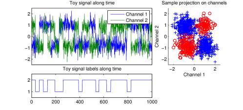
Figure 1: Toy example for $\sigma_{n}=0.5,lag=0$. The plots on the left show the evolution of both channels and labels along time; the right plot shows the non-linear problem by projecting the samples on the channels.

We use a toy example that consists of a 2D non-linear problem which can be seen on Figure 1. Each class contains 2 modes, $(-1,-1)$ and $(1,1)$ for class 1 and $(-1,1)$ and $(1,-1)$ for class 2, and their value is corrupted by a Gaussian noise of deviation $\sigma_{n}$. Moreover, the length of the regions with constant label follows a uniform distribution between $[30,40]$ samples. A time-lag drawn from a uniform distribution between $[-lag,lag]$ is applied to the channels leading to mislabeled samples in the learning and test set.

We illustrate the behavior of the large margin filtering on a simple example ($\sigma_{n}=1,lag=5$). The bivariate histogram of the projection of the samples on the channels can be seen on Figure 2. We can see on Figure 2(a) that due to the noise and time-lag there is an important overlap between the bivariate histograms of both classes, but when the large margin filter is applied, the classes are better separated (Figure 2(b)) and the overlap is reduced leading to better classification rate (4% error vs 40%).

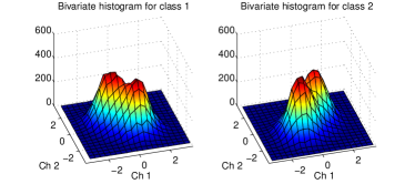
(a) Without filtering (err=0.404)

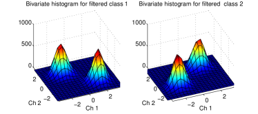
(b) With KF-SVM filtering (err=0.044)

Figure 2: Bivariate histograms for a non filtered ($\sigma_{n}=1,lag=5$) and KF-SVM filtered signal (left for class 1 and right for class 2)

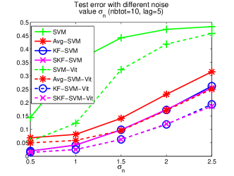
(a) varying noise value $\sigma_{k}$

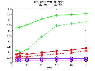
(b) varying size $nbtot$ of the problem

Figure 3: Test error for different problem size and noise for the toy example (plain lines : sample classification , dashed lines : Viterbi decoding)

SVM, Avg-SVM (signal filtered by average filter), KF-SVM and SKF-SVM are compared with and without Viterbi decoding. In order to test high dimensional problems, some channels containing only gaussian noise are added to the 2 discriminative ones leading to a toy signal of $nbtot$ channels. The size of the signal is of $1000$ samples for the learning and the validation sets and of $10000$ samples for the test set. In order to compare fairly with Avg-SVM, we selected $f=11$ and $n_{0}=6$ corresponding to a good average filtering centered on the current sample. The regularization parameters are selected by a validation method. All the processes are run ten times, the test error is then the average over the runs.

We can see in Figure 3 the test error for different noise value $\sigma_{n}$and problem size $nbtot$. Both proposed methods outperform SVM and Avg-SVM with a Wilcoxon signed-rank test p-value$<0.01$. Note that results obtained with KF-SVM without Viterbi decoding are even better than those observed with SVM and Viterbi decoding. This is probably because as we said previously, HMM can not adapt to time-lags because the learned density estimation are biased. Surprisingly, the use of the sparse regularization does not statistically improve the results despite the intrinsic sparsity of the problem. This comes from the fact that the learned filters of both methods are sparse due to a numerical precision thresholding for KF-SVM with Frobenius regularizer. Indeed the $\lambda$ coefficient selected by the validation is large, leading to a shrinkage of the non-discriminative channels.

We discuss the importance of the choice of our model parameters. In fact KF-SVM has 4 important parameters that have to be tuned: $\sigma_{k}$, $C$, $\lambda$ and $f$. Those parameters have to be tuned in order to fit the problem at hand. Note that $\sigma_{k}$ and $C$ are parameters linked to the SVM approach and that the remaining ones are due to the filtering approach. In the results presented below, a validation has been done to select $\lambda$ and $C$.

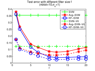
(a) varying f

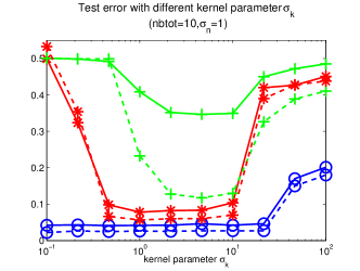
(b) varying sigma

Figure 4: Test error for different parameters on the toy example (plain lines : sample classification , dashed lines : Viterbi decoding)

We can see on the left of Figure 4 the performances of the different models for a varying $f$. Note that $f$ has a big impact on the performances when using Avg-SVM. On the contrary, KF-SVM shows good performances for a sufficiently long filter, due to the learning of the filtering. Our approach is then far less sensitive to the size of the filter than Avg-SVM. Finally we discuss the sensitivity to the kernel parameter $\sigma_{k}$. Test errors for different values of this parameters are shown on Figure 4 (right). It is interesting to note that KF-SVM is far less sensitive to this parameter than the other methods. Simply because the learning of the filtering corresponds to an automated scaling of the channels which means that if the $\sigma_{k}$ is small enough the scaling of the channels will be done automatically. In conclusion to these results, we can say that despite the fact that our method has more parameters to tune than a simple SVM approach, it is far less sensitive to two of these parameters than SVM.

4.2 BCI Dataset

We test our method on the BCI Dataset from BCI Competition III (Blankertz et al., , 2004). The problem is to obtain a sequence of labels out of brain activity signals for 3 human subjects. The data consists in 96 channels containing PSD features (3 training sessions, 1 test session, $n\approx{3000}$ per session) and the problem has 3 labels (left arm, right arm or a word).

For computational reasons, we decided to decimate the signal by 5, doing an averaging on the samples. We focus on online sample labeling ($n_{0}=0$) and we test KF-SVM for filter length $f$ corresponding to those used in (Flamary et al., , 2010). The regularization parameters are tuned using a grid search validation method on the third training set. Our method is compared to the best BCI competition results and to the SVM without filtering. Test error for different filter size $f$ can be seen on Table 1.

Method	Sub 1	Sub 2	Sub 3	Avg
BCI Comp.	0.2040	0.2969	0.4398	0.3135
SVM	0.2368	0.4207	0.5265	0.3947
KF-SVM
$f=2$	0.2140	0.3732	0.4978	0.3617
$f=5$	0.1840	0.3444	0.4677	0.3320
$f=10$	0.1598	0.2450	0.4562	0.2870

Table 1: Test Error for BCI Dataset

We can see that we improve the BCI Competition results by using longer filtering. We obtain similar results than those reported in Flamary et al., (2010) but slightly worst. This probably comes from the fact that the features used in this Dataset are PSD and are known to work well in the linear case. But we still obtain competitive results which is promising in the case of non-linear features.

5 Conclusions

We have proposed a framework for learning large-margin filtering for non-linear multi-channel sample labeling. Depending on the regularization term used, we can do either an adaptive scaling of the channels or a channels selection. We proposed a conjugate gradient algorithm to solve the minimization problem and empirical results showed that despite the non-convexity of the objective function our approach performs better than classical SVM methods. We tested our approach on a non-linear toy example and on a real life BCI dataset and we showed that sample classification rate and precision after Viterbi decoding can be drastically improved. Furthermore we studied the sensitivity of our method to the regularization parameters.

In future work, we will study the use of prior information on the classification task. For instance when we know that the noise is in high frequencies then we could force the filtering to be a low-pass filter. In addition, we will address the problem of computational learning complexity as our approach is not suitable to large-scale problems.