Euclidean Distances, soft and spectral Clustering
on Weighted Graphs

Abstract

We define a class of Euclidean distances on weighted graphs, enabling to perform thermodynamic soft graph clustering. The class can be constructed form the “raw coordinates” encountered in spectral clustering, and can be extended by means of higher-dimensional embeddings (Schoenberg transformations). Geographical flow data, properly conditioned, illustrate the procedure as well as visualization aspects.

KEYWORDS: average commute time distance, metastability, migratory flow, multidimensional scaling, Schoenberg transformations, shortest-path distance, spectral clustering, thermodynamic clustering, quasi-symmetry

1 Introduction

In a nutshell (see e.g. Shi and Malik (2000); Ng, Jordan and Weiss (2002); von Luxburg (2007) for a review), spectral graph clustering consists in

1. constructing a features-based similarity or affinity matrix between $n$ objects

2. performing the spectral decomposition of the normalized affinity matrix, and representing the objects by the corresponding eigenvectors or raw coordinates

3. applying a clustering algorithm on the raw coordinates.

The present contribution focuses on (C) thermodynamic clustering (Rose et al. 1990; Bavaud 2009), an aggregation-invariant soft $K$-means clustering based upon Euclidean distances between objects. The latter constitute distances on weighted graphs, and are constructed from the raw coordinates (B), whose form happens to be justified from presumably new considerations on equivalence between vertices (Section 3.3). Geographical flow data illustrate the theory (Section 4). Once properly symmetrized, endowed with a sensible diagonal and normalized, flows define an exchange matrix (Section 2), that is an affinity matrix (A) which might be positive definite or not.

A particular emphasis is devoted to the definition of Euclidean distances on weighted graphs and their properties (Section 3). For instance, diffusive and chi-square distances are focused, that is zero between equivalent vertices. Commute-time and absorption distances are not focused, but their values between equivalent vertices possess an universal character. All these distances, whose relationships to the shortest-path distance on weighted graphs is partly elucidated, differ in the way eigenvalues are used to scale the raw coordinates. Allowing further Schoenberg transformations (Definition 3) of the distances still extends the class of admissible distances on graphs, by means of a high-dimensional embedding familiar in the Machine Learning community.

2 Preliminaries and notations

Consider $n$ objects, together with an exchange matrix $E=(e_{ij})$, that is a $n\times n$ non-negative, symmetric matrix, whose components add up to unity (Berger and Snell 1957). $E$ can be obtained by normalizing an affinity of similarity matrix, and defines the normalized adjacency matrix of a weighted undirected graph (containing loops in general), where $e_{ij}$ is the weight of edge $(ij)$ and $f_{i}=\sum_{j=1}^{n}e_{ij}$ is the relative degree or weight of vertex $i$, assumed strictly positive.

2.1 Eigenstructure

$P=(p_{ij})$ with $p_{ij}=e_{ij}/f_{i}$ is the transition matrix of a reversible Markov chain, with stationary distribution $f$. The $t$-step exchange matrix is $E^{(t)}=\Pi P^{t}$, where $\Pi$ is the diagonal matrix containing the weights $f$. In particular, assuming the chain to be regular (see e.g. Kijima 1997)

$$E^{(0)}=\Pi\qquad\qquad E^{(2)}=E\Pi^{-1}E\enspace.\qquad\qquad E^{(\infty)}=ff^{\prime}$$

$P$ is similar to the symmetric, normalized exchange matrix $\Pi^{-\frac{1}{2}}E\Pi^{-\frac{1}{2}}$ (see e.g. Chung 1997), and share the same eigenvalues $1=\lambda_{0}\geq\lambda_{1}\geq\lambda_{2}\geq\ldots\lambda_{n-1}\geq-1$. It is well-known that the second eigenvalue $\lambda_{1}$ attains its maximum value 1 iff the graph contains disconnected components, and $\lambda_{n-1}=-1$ iff the graph is bipartite. We note $U^{\prime}\Lambda U$ the spectral decomposition of the normalized exchange matrix, where $\Lambda$ is diagonal and contains the eigenvalues, and $U=(u_{i\alpha})$ is orthonormal and contains the normalized eigenvectors. In particular, $u_{0}=\sqrt{f}$ is the eigenvector corresponding to the trivial eigenvalue $\lambda_{0}=1$. Also, the spectral decomposition of higher-order exchange matrices reads $\Pi^{-\frac{1}{2}}E^{(t)}\Pi^{-\frac{1}{2}}=U\Lambda^{t}U^{\prime}$.

2.2 Hard and soft partitioning

A soft partition of the $n$ objects into $m$ groups is specified by a $n\times m$ membership matrix $Z=(z_{ig})$, whose components (obeying $z_{ig}\geq 0$ and $\sum_{g=1}^{m}z_{ig}=1$) quantify the membership degree of object $i$ in group $g$. The relative volume of group $g$ is $\rho_{g}=\sum_{i}f_{i}z_{ig}$. The components $\theta_{gh}=\sum_{i}f_{i}z_{ig}z_{ih}$ of the $m\times m$ matrix $\Theta=Z^{\prime}\Pi Z$ measure the overlap between groups $g$ and $h$. In particular, $\theta_{gg}/\rho_{g}\leq~{}1$ measures the hardness of group $g$. The components $a_{gh}=\sum_{ij}e_{ij}z_{ig}z_{jh}$ of the $m\times m$ matrix $A=Z^{\prime}EZ$ measure the association between groups $g$ and $h$.

A group $g$ can also be specified by the objects it contains, namely by the distribution $\pi^{g}$ with components $\pi_{i}^{g}=f_{i}z_{ig}/\rho_{g}$, obeying $\sum_{i}\pi_{i}^{g}=1$ by construction. The object-group mutual information

$$I(O,Z)=H(O)+H(Z)-H(O,Z)=-\sum_{i}f_{i}\ln f_{i}-\sum_{g}\rho_{g}\ln\rho_{g}+\sum_{ig}f_{i}z_{ig}\ln(f_{i}z_{ig})$$

measures the object-group dependence or cohesiveness (Cover and Thomas 1991).

A partition is hard if each object belongs to an unique group, that is if the memberships are of the form $z_{ig}=I(i\in g)$, or equivalently if $z_{ig}^{2}=z_{ig}$ for all $i,g$, or equivalently if $\theta_{gg}=\rho_{g}$ for all $g$, or still equivalently if the overall softness $H(Z|O)=H(Z)-I(O,Z)$ takes on its minimum value of zero.

Also, $H(O)\leq\ln n$, with equality iff $f_{i}=1/n$, that is if the graph is regular.

2.3 Spectral versus soft membership relaxation

In their presentation of the Ncut-driven spectral clustering, Yu and Shi (2003) (see also Nock et al. 2009) determine the hard $n\times m$ membership $Z$ maximizing

$$\epsilon[Z]=\sum_{g=1}^{m}\frac{a_{gg}}{\rho_{g}}=\sum_{g}\frac{a_{gg}}{\theta_{gg}}=\mbox{tr}(X^{\prime}EX)\qquad\qquad\mbox{where}\quad X[Z]=Z\>\Theta^{-\frac{1}{2}}[Z]$$

under the constraint $X^{\prime}\Pi X=I$. Relaxing the hardness and non-negativity conditions, they show the solution to be $\epsilon[Z_{0}]=1+\sum_{\alpha=1}^{m-1}\lambda_{\alpha}$, attained with an optimal “membership” of the form $Z_{0}=X_{0}R\Theta^{\frac{1}{2}}$ where $R$ is any orthonormal $m\times m$ matrix and $X_{0}=({\bf 1},x_{1},\ldots,x_{\alpha},\ldots,x_{m-1})$ is the $n\times m$ matrix formed by the unit vector followed by of the first raw coordinates (Sec. 3.3). The above spectral relaxation of the memberships, involving the eigenstructure of the normalized exchange matrix, completely differs from the soft membership relaxation which will be used in Section 3.2, preserving positivity and normalization of $Z$.

3 Euclidean distances on weighted graphs

3.1 Squared Euclidean distances

Consider a collection of $n$ objects together with an associated pairwise distance. A successful clustering consists in partitioning the objects into $m$ groups, such that the average distances between objects belonging to the same (different) group are small (large). The most tractable pairwise distance is, by all means, the squared Euclidean distance $D_{ij}=\sum_{c=1}^{q}(x_{ic}-x_{jc})^{2}$, where $x_{ic}$ is the coordinate of object $i$ in dimension $c$. Its virtues follow from Huygens principles

$$\sum_{j}p_{j}D_{ij}=D_{ip}+\Delta_{p}\qquad\qquad\Delta_{p}=\sum_{j}p_{j}D_{jp}=\frac{1}{2}\sum_{ij}p_{i}p_{j}D_{ij}$$ (1)

where $p_{i}$ represents a (possibly non positive) signed distribution, i.e. obeying $\sum_{i}p_{i}=1$, $D_{ip}$ is the squared Euclidean distance between $i$ and the centroid of coordinates $\bar{x}_{pc}=\sum_{i}p_{i}x_{ic}$, and $\Delta_{p}$ the average pairwise distance or inertia. Equations (1) are easily checked using the coordinates, although the latter do not explicitly appear in the formulas. To that extent, squared Euclidean distances enable a feature-free formalism, a property shared with the kernels of Machine Learning, and to the “kernel trick” of Machine Learning amounts an equivalent “distance trick” (Schölkopf 2000; Williams 2002), as expressed by the well-known Classical Multidimensional Scaling (MDS) procedure. Theorem 3.1 below presents a weighted version (Bavaud 2006), generalizing the uniform MDS procedure (see e.g. Mardia et al. 1979). Historically, MDS has been developed from the independent contributions of Schoenberg (1938b) and Young and Householder (1938). The algorithm has been popularized by Torgeson (1958) in Data Analysis.

Theorem 3.1 (weighted classical MDS)

The dissimilarity square matrix $D$ between $n$ objects with weights $p$ is a squared Euclidean distance iff the scalar product matrix $B=-\frac{1}{2}HDH^{\prime}$ is (weakly) positive definite (p.d.), where $H$ is the $n\times n$ centering matrix with components $h_{ij}=\delta_{ij}-p_{j}$. By construction, $B_{ij}=-\frac{1}{2}(D_{ij}-D_{ip}-D_{jp})$ and $D_{ij}=B_{ii}+B_{jj}-2B_{ij}$. The object coordinates can be reconstructed as $x_{i\beta}=\mu_{\beta}^{\frac{1}{2}}p_{i}^{-\frac{1}{2}}v_{i\beta}$ for $\beta=1,2,\ldots$, where the $\mu_{\beta}$ are the decreasing eigenvalues and the $v_{i\beta}$ are the eigenvectors occurring in the spectral decomposition $K=VMV^{\prime}$ of the weighted scalar product or kernel $K$ with components $K_{ij}=\sqrt{p_{i}p_{j}}B_{ij}$. This reconstruction provides the optimal low-dimensional reconstruction of the inertia associated to $p$

$$\Delta=\frac{1}{2}\sum_{ij}p_{i}p_{j}D_{ij}=\mbox{tr}(K)=\sum_{\beta\geq 1}\mu_{\beta}\enspace.$$

Also, the Euclidean (or not) character of $D$ is independent of the choice of $p$.

3.2 Thermodynamic clustering

Consider the overall objects weight $f$, defining a centroid denoted by $0$, together with $m$ soft groups defined by their distributions $\pi^{g}$ for $g=1,\ldots,m$, with associated centroids denoted by $g$. By (1), the overall inertia decomposes as

$$\Delta=\sum_{i}f_{i}D_{i0}=\sum_{ig}f_{i}z_{ig}D_{i0}=\sum_{g}\rho_{g}\sum_{i}\pi^{g}_{i}D_{i0}=\sum_{g}\rho_{g}[D_{g0}+\Delta_{g}]=\Delta_{B}+\Delta_{W}$$

where $\Delta_{B}[Z]=\sum_{g}\rho_{g}D_{g0}$ is the between-groups inertia, and $\Delta_{W}[Z]=\sum_{g}\rho_{g}\Delta_{g}$ the within-groups inertia. The optimal clustering is then provided by the $n\times m$ membership matrix $Z$ minimizing $\Delta_{W}[Z]$, or equivalently maximizing $\Delta_{B}[Z]$. The former functional can be shown to be concave in $Z$ (Bavaud 2009), implying the minimum to be attained for hard clusterings.

Hard clustering is notoriously computationally intractable and some kind of regularization is required. Many authors (see e.g. Huang and Ng (1999) or Filippone et al. (2008)) advocate the use of the $c$-means clustering, involving a power transform of the memberships. Despite its efficiency and popularity, the $c$-means algorithm actually suffers from a serious formal defect, questioning its very logical foundations: its objective function is indeed not aggregation-invariant, that is generally changes when two groups $g$ and $h$ supposed equivalent in the sense $\pi^{g}=\pi^{h}$ are merged into a single group $[g\cup h]$ with membership $z_{i[h\cup g]}=z_{ih}+z_{jh}$ (Bavaud 2009).

An alternative, aggregation-invariant regularization is provided by the thermodynamic clustering, minimizing over $Z$ the free energy $F[Z]=\Delta_{W}[Z]+TI[Z]$, where $I[Z]\equiv I(O,Z)$ is the objects-groups mutual information and $T>0$ the temperature (Rose et al. 1990; Rose 1998; Bavaud 2009). The resulting membership is determined iteratively through

$$z_{ig}=\frac{\rho_{g}\>\exp(-D_{ig}/T)}{\sum_{h=1}^{m}\rho_{h}\>\exp(-D_{ih}/T)}$$ (2)

and converges towards a local minimum of the free energy. Equation (2) amounts to fitting Gaussian clusters in the framework of model-based clustering.

3.3 Three nested classes of squared Euclidean distances

Equation (2) solves the K-way soft graph clustering problem, given of course the availability of a sound class of squared Euclidean distances on weighted graphs. Definitions 2 and 3 below seem to solve the latter issue.

Consider a graph possessing two distinct but equivalent vertices in the sense their relative exchange is identical with the other vertices (including themselves). Those vertices somehow stand as duplicates of the same object, and one could as a first attempt require their distance to be zero.

Definition 1 (Equivalent vertices; focused distances)

Two distinct vertices $i$ and $j$ are equivalent, noted $i\sim j$, if $e_{ik}/f_{i}=e_{jk}/f_{j}$ for all $k$. A distance is focused if $D_{ij}=0$ for $i\sim j$.

Proposition 1

$i\sim j$ iff $x_{i\alpha}=x_{j\alpha}$ for all $\alpha\geq 1$ such that $\lambda_{\alpha}\neq 0$, where $x_{i\alpha}=u_{i\alpha}/\sqrt{f_{i}}$ is the raw coordinate of vertex $i$ in dimension $\alpha$.

The proof directly follows from the substitution $e_{ik}\to f_{i}e_{jk}/f_{j}$ in the identity $\sum_{k}f_{i}^{-\frac{1}{2}}e_{ik}f_{k}^{-\frac{1}{2}}u_{k\alpha}=\lambda_{\alpha}u_{i\alpha}$. Note that the condition trivially holds for the trivial eigenvector $\alpha=0$, in view of $f_{i}^{-\frac{1}{2}}u_{i0}\equiv 1$ for all $i$. It also holds trivially for the “completely connected” weighted graph $e_{ij}^{(\infty)}=f_{i}f_{j}$, where all vertices are equivalent, and all eigenvalues are zero, except the trivial one.

Hence, any expression of the form $D_{ij}=\sum_{\alpha\geq 1}g_{\alpha}(f_{i}^{-\frac{1}{2}}u_{i\alpha}-f_{j}^{-\frac{1}{2}}u_{j\alpha})^{2}$ with $g_{\alpha}\geq 0$ constitutes an admissible squared Euclidean distance, obeying $D_{ij}=0$ for $i\sim j$, provided $g_{\alpha}=0$ if $\lambda_{\alpha}=0$. The quantities $g_{\alpha}$ are non-negative, but otherwise arbitrary; however, it is natural to require the latter to depend upon the sole parameters at disposal, namely the eigenvalues, that is to set $g_{\alpha}=g(\lambda_{\alpha})$.

Definition 2 (Focused and Natural Distances on Weighted Graphs)

Let $E$ be the exchange matrix associated to a weighted graph, and define $E^{s}:=\Pi^{-\frac{1}{2}}(E-E^{(\infty)})\Pi^{-\frac{1}{2}}$, the standardized exchange matrix. The class of focused squared Euclidean distances on weighted graphs is

$$D_{ij}=B_{ii}+B_{jj}-2B_{ij},\quad\mbox{where}\quad B=\Pi^{-\frac{1}{2}}K\Pi^{-\frac{1}{2}}\quad\mbox{and}\quad K=g(E^{s})$$

where $g(\lambda)$ is any non-negative sufficiently regular real function with $g(0)=0$. Dropping the requirement $g(0)=0$ defines the more general class of natural squared Euclidean distances on weighted graphs.

If $g(1)$ is finite, $K$ can also be defined as $K=g(\Pi^{-\frac{1}{2}}E\Pi^{-\frac{1}{2}})=Ug(\Lambda)U^{\prime}$.

First, note the standardized exchange matrix to result from a “centering” (eliminating the trivial eigendimension) followed by a “normalization”:

$$e_{ij}^{s}=\frac{e_{ij}-f_{i}f_{j}}{\sqrt{f_{i}f_{j}}}=\sum_{\alpha\geq 1}\lambda_{\alpha}u_{i\alpha}u_{j\alpha}\enspace.$$ (3)

Secondly, $B$ is the matrix of scalar products appearing in Theorem 3.1. The resulting optimal reconstruction coordinates are $\sqrt{g(\lambda_{\alpha})}\>x_{i\alpha}$, where the quantities $x_{i\alpha}=f_{i}^{-\frac{1}{2}}u_{i\alpha}$ are the raw coordinates of vertex $i$ in dimension $\alpha=1,2,\ldots$ appearing in Proposition 1 - which yields a general rationale for their widespread use in clustering and low-dimensional visualization. Thirdly, the matrix $g(E^{s})$ can be defined, for $g(\lambda)$ regular enough, as the power expansion in $(E^{s})^{t}$ with coefficients given by the power expansion of $g(\lambda)$ in $\lambda^{t}$, for $t=0,1,2,\ldots$. Finally, the two variants of $B$ appearing in Definition 2 are identical up to a matrix $g(1){\bf 1}_{n}{\bf 1}_{n}^{\prime}$, leaving $D$ unchanged.

If $g(1)=\infty$, the distance between vertices belonging to distinct irreducible components becomes infinite: recall the graph to be disconnected iff $\lambda_{1}=1$. Such distances will be referred to as irreducible.

Natural distances are in general not focused. The distances between equivalent vertices are however universal, that is independent of the details of the graph or of the associated distance (Proposition 2). To demonstrate this property, consider first an equivalence class $J:=\{k\>|\>k\sim j\}$ containing at least two equivalent vertices. Aggregating the vertices in $J$ results in a new $\tilde{n}\times\tilde{n}$ exchange matrix $\tilde{E}$ with $\tilde{n}=(n-|J|-1)$, with components $\tilde{e}_{JJ}=\sum_{ij\in J}e_{ij}$, $\tilde{e}_{Jk}=\tilde{e}_{kJ}=\sum_{j\in J}e_{jk}$ for $k\notin J$ and $\tilde{f}_{J}=\sum_{j\in J}f_{j}$, the other components remaining unchanged.

Proposition 2

Let $D$ be a natural distance and consider a graph possessing an equivalence class $J$ of size $|J|\geq 2$. Consider two distinct elements $i\sim j$ of $J$ and let $k\notin J$. Then

$$D_{ij}=g(0)\>(\frac{1}{f_{i}}+\frac{1}{f_{j}})\qquad\qquad D_{jJ}=g(0)\>(\frac{1}{f_{i}}-\frac{1}{\tilde{f}_{J}})\qquad\qquad\Delta_{J}=g(0)\>\frac{|J|-1}{\tilde{f}_{J}}\enspace.$$

Moreover, the Pythagorean relation $D_{kj}=D_{kJ}+D_{jJ}$ holds.

Proof: consider the eigenvalues $\tilde{\lambda}_{\beta}$ and eigenvectors $\tilde{u}_{\beta}$, associated to the aggregated graph $\tilde{E}$, for $\beta=0,\ldots,\tilde{n}$. One can check that, due to the collinearity generated by the $|J|$ equivalent vertices,

1. $\tilde{n}$ among the original eigenvalues $\lambda_{\alpha}$ coincide with the set of aggregated eigenvalues $\tilde{\lambda}_{\beta}$ (non null in general), with corresponding eigenvectors $u_{j\beta}=f_{j}^{\frac{1}{2}}\tilde{f}_{J}^{-\frac{1}{2}}\tilde{u}_{J\beta}$ for $j\in J$ and $u_{k\beta}=\tilde{u}_{k\beta}$ for $k\notin J$

2. $|J-1|$ among the original eigenvalues $\lambda_{\alpha}$ are zero. Their corresponding eigenvectors are of the form $u_{j\gamma}=h_{j\gamma}$ for $j\in J$ and $u_{k\gamma}=0$ for $k\notin J$, where the $h_{\gamma}$ constitute the $|J|-1$ columns of an orthogonal $|J|\times|J|$ matrix, the remaining column being $(f_{j}^{\frac{1}{2}}\tilde{f}^{-^{\frac{1}{2}}}_{J})_{j\in J}$.

Identities in Proposition 2 follow by substitution. For instance,

$$D_{ij}=\sum_{\beta=1}^{\tilde{n}}g(\lambda_{\beta})(\frac{u_{i\beta}}{\sqrt{f_{i}}}-\frac{u_{j\beta}}{\sqrt{f_{j}}})^{2}+g(0)\sum_{\gamma=1}^{|J|-1}(\frac{h_{i\gamma}}{\sqrt{f_{i}}}-\frac{h_{j\gamma}}{\sqrt{f_{j}}})^{2}=g(0)\>(\frac{1}{f_{i}}+\frac{1}{f_{j}})\enspace.$$

General at it is, the class of squared Euclidean distances on weighted graphs of Definition 2 can still be extended: a wonderful result of Schoenberg (1938a), still apparently little known in the Statistical and Machine Learning community (see however the references in Kondor and Lafferty (2002); Hein et al. (2005)) asserts that the componentwise correspondence $\tilde{D}_{ij}=\phi(D_{ij})$ transforms any squared Euclidean distance $D$ into another squared Euclidean distance $\tilde{D}$, provided that

1. $\phi(D)$ is positive with $\phi(0)=0$

2. odd derivatives $\phi^{\prime}(D)$, $\phi^{\prime\prime\prime}(D)$,… are positive

3. even derivatives $\phi^{\prime\prime}(D)$, $\phi^{\prime\prime\prime\prime}(D)$,… are negative.

For example, $\phi(D)=D^{a}$ (for $0<a\leq 1$) and $\phi(D)=1-\exp(-bD)$ (for $b>0$) are instances of such Schoenberg transformations (Bavaud 2010).

Definition 3 (Extended Distances on Weighted Graphs)

The class of extended squared Euclidean distances on weighted graphs is

$$\tilde{D}_{ij}=\phi(D_{ij})$$

where $\phi(D)$ is a Schoenberg transformation (as specified above), and $D_{ij}$ is a natural squared Euclidean distance associated to the weighted graph $E$, in the sense of Definition 2.

3.4 Examples of distances on weighted graphs

3.4.1 The chi-square distance

The choice $g(\lambda)=\lambda^{2}$ entails, together with (3)

$$\Delta=\mbox{tr}(K)=\mbox{tr}((E^{s})^{2})=\sum_{ij}\frac{(e_{ij}-f_{i}f_{j})^{2}}{f_{i}f_{j}}=\chi^{2}$$

which is the familiar chi-square measure of the overall rows-columns dependency in a (square) contingency table, with distance $D^{\chi}_{ij}=\sum_{k}f_{k}^{-1}(f_{i}^{-1}e_{ik}-f_{j}^{-1}e_{jk})^{2}$, well-known in the Correspondence Analysis community (Lafon and Lee 2006; Greenacre 2007 and references therein). Note that $D^{\chi}_{ij}=0$ for $i\sim j$, as it must.

3.4.2 The diffusive distance

The choice $g(\lambda)=\lambda$ is legitimate, provided the exchange matrix is purely diffusive, that is p.d. Such are typically the graphs resulting from inter-regional migrations (Sec. 4) or social mobility tables (Bavaud 2008). As most people do not change place or status during the observation time, the exchange matrix is strongly dominated by its diagonal, and hence p.d.

Positive definiteness also occurs for graphs defined from the affinity matrix $\exp(-\beta D_{ij})$ (Gaussian kernel), as in Belkin and Niyogi (2003), among many others. Indeed, distances derived from the Gaussian kernel provide a prototypical example of Schoenberg transformation (see Definition 3). By contrast, the affinity $I(D_{ij}\leq~{}\epsilon^{2})$ used by Tenenbaum et al. (2000) is not p.d.

The corresponding distance, together with the inertia, plainly read

$$D^{\mbox{\small\it dif}}_{ij}=\frac{e_{ii}}{f_{i}^{2}}+\frac{e_{jj}}{f_{j}^{2}}-2\frac{e_{ij}}{f_{i}f_{j}}\qquad\qquad\Delta^{\mbox{\small\it dif}}=\sum_{i}\frac{e_{ii}}{f_{i}}-1\enspace.$$

3.4.3 The “frozen” distance

The choice $g(\lambda)\equiv 1$ produces, for any graph, a result identical to the application of any function $g(\lambda)$ (with $g(1)=1$) to the purely diagonal “frozen” graph $E^{(0)}=\Pi$, namely (compare with Proposition 2):

$$D_{ij}^{\mbox{\small\it fro}}=\frac{1}{f_{i}}+\frac{1}{f_{j}}\quad\mbox{for $i\neq j$}\qquad\qquad D_{i0}^{\mbox{\small\it fro}}=\frac{1}{f_{i}}-1\qquad\qquad\Delta^{\mbox{\small\it fro}}=n-1\enspace.$$

This “star-like” distance (Critchley and Fichet 1994) is embeddable in a tree.

3.4.4 The average commute time distance

The choice $g(\lambda)=(1-\lambda)^{-1}$ corresponds to the average commute time distance; see Fouss et al. (2007) for a review and recent results. The amazing fact that the latter constitutes a squared Euclidean distance has only be recently explicitly recognized as such, although the key ingredients were at disposal ever since the seventies.

Let us sketch a derivation of this result: on one hand, consider a random walk on the graph with probability transition matrix $P=\Pi^{-1}E$, and let $T_{j}$ denotes the first time the chain hits state $j$. The average time to go from $i$ to $j$ is $m_{ij}=E_{i}(T_{j})$, with $m_{ii}=0$, where $E_{i}(.)$ denotes the expectation for a random walk started in $i$. Considering the state following $i$ yields for $i\neq j$ the relation $m_{ij}=1+\sum_{k}p_{ik}m_{kj}$, with solution (Kemeny and Snell (1976); Aldous and Fill, draft chapters) $m_{ij}=(y_{jj}-y_{ij})/f_{j}$, where $Y=\Pi^{-1}\sum_{t\geq 0}(E^{(t)}-E^{(\infty)})=(E^{(0)}-E+E^{(\infty)})^{-1}\Pi$ is the so-called fundamental matrix of the Markov chain. On the other hand, Definition 2 yields $K=(I-E^{s})^{-1}=\Pi^{\frac{1}{2}}(E^{(0)}-E+E^{(\infty)})^{-1}\Pi^{\frac{1}{2}}=\Pi^{\frac{1}{2}}Y\Pi^{-\frac{1}{2}}$, and thus $B=Y\Pi^{-1}=\Pi^{-1}Y$. Hence

$$D^{\mbox{\small\it com}}_{ij}=B_{ii}+B_{jj}-2B_{ij}=\frac{y_{ii}}{f_{i}}+\frac{y_{jj}}{f_{j}}-\frac{y_{ij}}{f_{j}}-\frac{y_{ij}}{f_{j}}=m_{ij}+m_{ji}$$

which is the average time to go from $i$ to $j$ and back to $i$, as announced.

Consider, for future use, the Dirichlet form ${\cal E}(y)=\frac{1}{2}\sum_{ij}e_{ij}(y_{i}-y_{j})^{2}$, and denote by $y^{0}$ the solution of the “electrical” problem $\min_{y\in C_{ij}}{\cal E}(y)$, where $C_{ij}$ denotes the set of vectors $y$ such that $y_{i}=1$ and $y_{j}=0$. Then $y_{k}^{0}=P_{k}(T_{i}<T_{j})$, where $P_{k}(.)$ denotes the probability for a random walk started at $k$. Then $D^{\mbox{\small\it com}}_{ij}=1/{\cal E}(y^{0})$ (Aldous and Fill, chapter 3).

3.4.5 The shortest-path distance

Let $\Gamma_{ij}$ be the set of paths with extremities $i$ and $j$, where a path $\gamma\in\Gamma_{ij}$ consists of a succession of consecutive unrepeated edges denoted by $\alpha=(k,l)\in\gamma$, whose weights $e_{\alpha}$ represent conductances. Their inverses are resistances, whose sum is to be minimized by the shortest path $\gamma^{0}\in\Gamma_{ij}$ (not necessarily unique) on the weighted graph $E$. This setup generalizes the unweighted graphs framework, and defines the shortest path distance

$$D^{\mbox{\small\it sp}}_{ij}=\min_{\gamma\in\Gamma_{ij}}\sum_{\alpha\in\gamma}\frac{1}{e_{\alpha}}\enspace.$$

We believe the following result to be new - although its proof simply combines a classical result published in the fifties (Beurling and Deny 1958) with the above “electrical” characterization of the average commute time distance.

Proposition 3

$D^{\mbox{\small\it sp}}_{ij}\geq D^{\mbox{\small com}}_{ij}$ with equality for all $i,j$ iff $E$ is a weighted tree.

Proof: let $\gamma^{0}\in\Gamma_{ij}$ be the shortest-path between $i$ and $j$. Consider a vector $y$ and define $dy_{\alpha}=y_{l}-y_{k}$ for an edge $\alpha=(k,l)$. Then

$$|y_{i}-y_{j}|\stackrel{{\scriptstyle(a)}}{{\leq}}\sum_{\alpha\in\gamma^{0}}|dy_{\alpha}|=\sum_{\alpha\in\gamma^{0}}\sqrt{e_{\alpha}}\frac{|dy_{\alpha}|}{\sqrt{e_{\alpha}}}\stackrel{{\scriptstyle(b)}}{{\leq}}(\sum_{\alpha\in\gamma^{0}}e_{\alpha}(dy_{\alpha})^{2})^{\frac{1}{2}}(\sum_{\alpha\in\gamma^{0}}\frac{1}{{e_{\alpha}}})^{\frac{1}{2}}\stackrel{{\scriptstyle(c)}}{{\leq}}\sqrt{{\cal E}(y)}\sqrt{D^{\mbox{\small\it sp}}_{ij}}$$

Hence $D^{\mbox{\small\it sp}}_{ij}\geq(y_{i}-y_{j})^{2}/{\cal E}(y)$ for all $y$, in particular for $y^{0}$ defined above, showing $D^{\mbox{\small\it sp}}_{ij}\geq D^{\mbox{\small\it com}}_{ij}$. Equality holds iff (a) $y^{0}$ is monotonously decreasing along the path $\gamma^{0}$, (b) for all $\alpha\in\gamma^{0}$, $dy^{0}_{\alpha}=c/e_{\alpha}$ for some constant $c$, and (c) $dy^{0}_{\alpha}e_{\alpha}=0$ for all $\alpha\notin\gamma^{0}$. (b), expressing Ohm’s law $U=RI$ in the electrical analogy, holds for $y^{0}$, and (a) and (c) hold for a tree, that is a graph possessing no closed path.

The shortest-path distance is unfocused and irreducible. Seeking to determine the corresponding function $g(\lambda)$ involved in Definition 2, and/or the Schoenberg transformation $\phi(D)$ involved in Definition 3, is however hopeless:

Proposition 4

$D^{\mbox{\small\it sp}}$ is not a squared Euclidean distance.

Proof: a counter-example is provided (Deza and Laurent (1997) p. 83) by the complete bipartite graph $K_{2,3}$ of Figure 1:

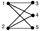
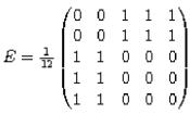
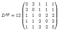
Figure 1: Bipartite graph $K_{2,3}$, associated exchange matrix and shortest-path distance

The eigenvalues occurring in Theorem 3.1 are $\mu_{1}=3$, $\mu_{2}=2.32$, $\mu_{3}=2$, $\mu_{4}=0$ and ${\mathbf{\mu_{5}=-0.49}}$, thus ruling out the possible squared Euclidean nature of $D^{\mbox{\small\it sp}}$.

3.4.6 The absorption distance

The choice $g(\lambda)=(1-\rho)/(1-\rho\lambda)$ where $0<\rho<1$ yields the absorption distance: consider a modified random walk, where, at each discrete step, a particle at $i$ either undergoes with probability $\rho$ a transition $i\to j$ (with probability $p_{ij}$) or is forever absorbed with probability $1-\rho$ into some additional “cemetery” state. The quantities $v_{ij}(\rho)$ = “ average number of visits from $i$ to $j$ before absorption” obtain as the components of the matrix (see e.g. Kemeny and Snell (1976) or Kijima (1997))

$$V(\rho)=(I-\rho P)^{-1}=(\Pi-\rho E)^{-1}\Pi\>\>\mbox{with}\>\>f_{i}v_{ij}=f_{j}v_{ji}\>\>\mbox{and}\>\>\sum_{i}f_{i}v_{ij}=\frac{f_{j}}{1-\rho}\enspace.$$

Hence $K=g(\Pi^{-\frac{1}{2}}E\Pi^{-\frac{1}{2}})=(1-\rho)\Pi^{\frac{1}{2}}V\Pi^{-\frac{1}{2}}$ and $B_{ij}=(1-\rho)v_{ij}/f_{j}$, measuring the ratio of the average number of visits from $i$ to $j$ over its expected value over the initial state $i$. Finally,

$$D_{ij}^{\mbox{\small\it abs}}(\rho)=\frac{v_{ii}(\rho)}{f_{i}}+\frac{v_{jj}(\rho)}{f_{j}}-2\frac{v_{ij}(\rho)}{f_{j}}\enspace.$$

By construction, $\lim_{\rho\to 0}D^{\mbox{\small\it abs}}(\rho)=D^{\mbox{\small\it fro}}$ and $\lim_{\rho\to 1}(1-\rho)^{-1}D^{\mbox{\small\it abs}}(\rho)=D^{\mbox{\small\it com}}$. Also, $\lim_{\rho\to 1}D^{\mbox{\small\it abs}}(\rho)\equiv 0$ for a connected graph.

3.4.7 The “sif” distance

The choice $g(\lambda)=\lambda^{2}/(1-\lambda)$ is the simplest one insuring an irreducible and focused squared Euclidean distance. Identity $\lambda^{2}/(1-\lambda)=1/(1-\lambda)-\lambda-1$ readily yields (wether $D^{\mbox{\small\it dif}}$ is Euclidean or not)

$$D^{\mbox{\small\it sif}}_{ij}=D^{\mbox{\small\it com}}_{ij}-D^{\mbox{\small\it dif}}_{ij}-D^{\mbox{\small\it fro}}_{ij}\enspace.$$

4 Numerical experiments

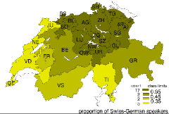
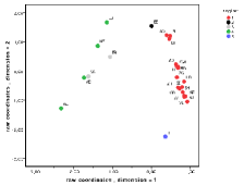
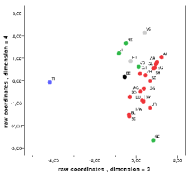
Figure 2: Proportion of Swiss-German speakers in the 26 Swiss cantons (left), and raw coordinates $x_{i\alpha}$ associated to the inter-cantonal migrations, in dimensions $\alpha=1,2$ (center) and $\alpha=3,4$ (right). Colours code the linguistic regions, namely: 1 = German, 2 = mainly German, 3 = mainly French, 4 = French and 5 = Italian. The central factorial map reconstructs fairly precisely the geographical map, and emphasizes the linguistic German-French barrier, known as “Röstigraben”. The linguistic isolation of the sole Italian-speaking canton, intensified by the Alpine barrier, is patent.

4.1 Inter-cantonal migration data

The first data set consists of the numbers $N=(n_{ij})$ of people inhabiting the Swiss canton $i$ in 1980 and the canton $j$ in 1985 ($i,j=1,\ldots,n=26$), with a total count of $6^{\prime}039^{\prime}313$ inhabitants, $93\%$ of which are distributed over the diagonal. $N$ can be made brutally symmetric as $\frac{1}{2}(n_{ij}+n_{ji})$ or $\sqrt{n_{ij}n_{ji}}$, or, more gently, by fitting a quasi-symmetric model (Bavaud 2002), as done here. Normalizing the maximum likelihood estimate yields the exchange matrix $E$. Raw coordinates $x_{i\alpha}=u_{i\alpha}/\sqrt{f_{i}}$ are depicted in Figure 2. By construction, they do not depend of the form of the function $g(\lambda)$ involved in Definition 2, but they do depend on the form of the Schoenberg transformation $\tilde{D}=\phi(D)$ involved in Definition 3, where they obtain as solutions of the weighted MDS algorithm (Theorem 3.1) on $\tilde{D}$, with unchanged weights $f$ (Figure 3 (a) and (b)).

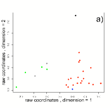
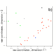
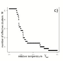
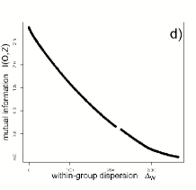
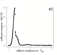
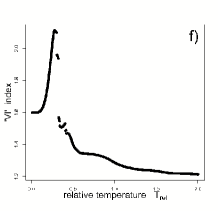
Figure 3: Raw coordinates extracted from weighted MDS after applying Schoenberg transformations $\tilde{D}=\phi(D^{\mbox{\tiny\it com}})$ with $\phi(D)=D^{0.7}$ (a), and $\phi(D)=1-\exp(-bD)$ with $b=1/(4\Delta^{\mbox{\tiny\it com}})$ (b). Decrease of the number of effective groups with the temperature (c); beside the main component, two microscopic groups of size $\rho_{2}=6\cdot 10^{-4}$ and $\rho_{3}=2\cdot 10^{-45}$ survive at $T_{\mbox{\tiny rel}}=2$. (d) is the so-called rate-distortion function of Information Theory; its discontinuity at $T_{\mbox{\tiny crit}}=0.406$ betrays a phase transition between a cold regime with numerous clusters and a hot regime with few clusters (Rose et al. 1990; Bavaud 2009). Behaviour of the overall softness $H(Z|O)$ (e) (Section 2.2) and of the clusters-regions variation of information (f) (see text).

Iterating (2) from an initial $n\times m$ membership matrix $Z_{\mbox{\tiny init}}$ (with $m\leq n$) at fixed $T$ yields a membership $Z_{0}(T)$, which is by construction a local minimizer of the free energy $F[Z,T]$. The number $M(Z_{0})\leq m$ of independent columns of $Z_{0}$ measures the number of effective groups: equivalent groups, that is groups whose columns are proportional, could and should be aggregated, thus resulting in $M$ distinct groups, without changing the free energy, since both the intra-group dispersion and the mutual information are aggregation-invariant (Bavaud 2009). In practice, groups $g$ and $h$ are judged as equivalent if their relative overlap (Section 2.2) obeys $\theta_{gh}/\sqrt{\theta_{gg}\theta_{hh}}\geq 1-10^{-10}$.

Define the relative temperature as $T_{\mbox{\tiny rel}}=T/\Delta$. One expects $M=1$ for $T_{\mbox{\tiny rel}}\gg 1$, and $M=n$ for $T_{\mbox{\tiny rel}}\ll 1$, provided of course that the initial membership matrix contains at least $n$ columns. We operate a soft hierarchical descendant clustering scheme, consisting in starting with the identity membership $Z_{\mbox{\tiny init}}=I$ for some $T_{\mbox{\tiny rel}}\ll 1$, iterating (2) until convergence, and then aggregating the equivalent columns in $Z_{0}(T)$ into $M$ effective groups. The temperature is then slightly increased, and, choosing the resulting optimum $Z_{0}(T)$ as the new initial membership, (2) is iterated again, and so forth until the emergence of a single effective group ($M=1$) in the high temperature phase $T_{\mbox{\tiny rel}}\geq 1$.

Numerical experiments (Figure 3) actually conform to the above expectations, yet with an amazing propensity for tiny groups $\rho_{g}\ll 1$ to survive at high temperature, that is before to be aggregated in the main component. This metastable behaviour is related to the locally optimal nature of the algorithm; presumably unwanted in practical applications, it can be eliminated by forcing group coalescence if, for instance, $H(Z)$ or $F[Z]-\Delta$ become small enough.

The softness measure of the clustering $H(Z|O)$ is expected to be zero in both temperature limits, since both the identity matrix and the single-group membership matrix are hard. We have attempted to measure the quality of the clustering $Z$ with respect to the regional classification $R$ of Figure 2 by the “variation of information” index $H(Z)+H(R)-2I(Z,R)$ proposed by Meila (2005). Further investigations, beyond the scope of this paper, are obviously still to be conducted in this direction.

The stability of the effective number of clusters around $T_{\mbox{\tiny rel}}=1$ might encourage the choice of the solution with $M=7$ clusters. Rather disappointingly, the latter turns out (at $T_{\mbox{\tiny rel}}=0.8$, things becoming even worse at higher temperature) to consist of one giant main component of $\rho_{1}>0.97$, together with 6 other practically single-object groups (UR, OW, NW, GL, AI, JU), totalizing less than three percent of the total mass (see also Section 5).

4.2 Commuters data

The second data set counts the number of commuters $N=n_{ij}$ between the $n=892$ French speaking Swiss communes, living in commune $i$ and working in commune $j$ in 2000. A total of $733^{\prime}037$ people are involved, $49\%$ of which are distributed over the diagonal. As before, the exchange matrix $E$ is obtained after fitting a quasi-symmetric model to $N$.

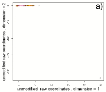
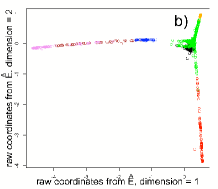
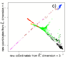
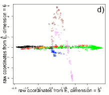
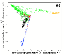
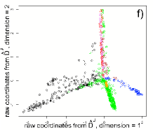
Figure 4: Raw coordinates associated to the unmodified exchange matrix $E$ are unable to approximate the geographical map (a), in contrast to (b), (c) and (d), based upon the diagonal-free exchange matrix $\hat{E}$. Colours code the cantons, namely BE=brown, FR=black, GE=orange, JU=violet, NE=blue, VD=green, VS=red. In particular, the central position of VD (compare with Figure 2) is confirmed. (e) and (f) represent the low-dimensional coordinates obtained by MDS from $\hat{D}^{\mbox{\tiny\it jump}}$ (4).

The first two dimensions $\alpha=1,2$ of the raw coordinates $x_{i\alpha}=u_{i\alpha}/\sqrt{f_{i}}$ are depicted in Figure 4 a). The objects cloud consists of all the communes (up, left) except a single one (down, right), namely “Roche d’Or” (JU), containing 15 active inhabitants, 13 of which work in Roche d’Or. Both the very high value of the proportion of stayers $e_{ii}/f_{i}$ and the low value of the weight $f_{i}$ make Roche d’Or (together with other communes, to a lesser extent) quasi-disconnected from the rest of the system, hence producing, in accordance to the theory, eigenvalues as high as $\lambda_{1}=.989$, $\lambda_{2}=.986$, … , $\lambda_{30}>.900$…

Theoretically flawless as is might be, this behavior stands as a complete geographical failure. As a matter of fact, commuters (and migration)-based graphs are young, that is $E$ is much closer to its short-time limit $E^{(0)}$ than to its equilibrium value $E^{(\infty)}$. Consequently, diagonal components are huge and equivalent vertices in the sense of Definition 1 cannot exist: for $k=i\neq j$, the proportion of stayers $e_{ii}/f_{i}$ is large, while $e_{ij}/f_{j}$ is not.

Attempting to consider the Laplacian $E-E^{(0)}$ instead of $E$ does not improve the situation: both matrices indeed generate the same eigenstructure, keeping the order of eigenvalues unchanged. A brutal, albeit more effective strategy consists in plainly destroying the diagonal exchanges, that is by replacing $E$ by the diagonal-free exchange matrix $\hat{E}$, with components and associated weights

$$\hat{e}_{ij}=\frac{e_{ij}-\delta_{ij}e_{ii}}{1-\sum_{k}e_{kk}}\qquad\qquad\qquad\hat{f}_{i}=\frac{f_{i}-e_{ii}}{1-\sum_{k}e_{kk}}\enspace.$$

Defining $\hat{E}$ as the new exchange matrix yields (Sections 2 and 3) new weights $\hat{f}$, eigenvectors $\hat{U}$, eigenvalues $\hat{\Lambda}$ (with $\hat{\lambda}_{n}=0$), raw coordinates $\hat{X}$ and distances $\hat{D}$, as illustrated in Figure 4 b), c) and d).

However, an example of equivalent nodes in the sense of Definition 1 is still unlikely to be found, since $0=\hat{e}_{ii}/\hat{f}_{i}\neq\hat{e}_{ij}/\hat{f}_{j}$ in general. A weaker concept of equivalence consists in comparing $i\neq j$ by means of their transition probabilities towards the other vertices $k\neq i,j$, that is by means of the Markov chain conditioned to the event that the next state is different. Such Markov transitions approximate the so-called jump process, if existing (see e.g. Kijima (1997) or Bavaud (2008)). Their associated exchange matrix is precisely given by $\hat{E}$.

Definition 4 (Weakly equivalent vertices; weakly focused distances)

Two distinct vertices $i$ and $j$ are weakly equivalent, noted $i\stackrel{{\scriptstyle w}}{{\sim}}j$, if $\hat{e}_{ik}/\hat{f}_{i}=\hat{e}_{jk}/\hat{f}_{j}$ for all $k\neq i,j,$. A distance is weakly focused if $D_{ij}=0$ whenever $i\stackrel{{\scriptstyle w}}{{\sim}}j$.

By construction, the following “jump” distance is squared Euclidean and weakly focused:

$$\hat{D}^{\mbox{\small\it jump}}_{ij}=\sum_{k\>|\>k\neq i,j}\hat{f}_{k}(\frac{\hat{e}_{ik}}{\hat{f}_{i}\hat{f}_{k}}-\frac{\hat{e}_{jk}}{\hat{f}_{j}\hat{f}_{k}})^{2}=\sum_{k}\frac{1}{\hat{f}_{k}}(\frac{\hat{e}_{ik}}{\hat{f}_{i}}-\frac{\hat{e}_{jk}}{\hat{f}_{j}})^{2}-\frac{\hat{e}_{ij}^{2}}{\hat{f}_{i}\hat{f}_{j}}(\frac{1}{\hat{f}_{i}}+\frac{1}{\hat{f}_{j}})\enspace.$$ (4)

The restriction $k\neq i,j$ in (4) complicates the expression of $D^{\mbox{\small\it jump}}$ in terms of the eigenstructure $(\hat{U},\hat{\Lambda})$, and the existence of raw coordinates $\hat{x}_{i\alpha}$, adapted to the diagonal-free case, and justified by an analog of Proposition 1, remains open. In any case, jump distances (4) are well defined, and yield low-dimensional coordinates of the 892 communes by weighted MDS (Theorem 3.1) with weights $\hat{f}$, as illustrated in Figure 4 e) and f).

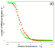
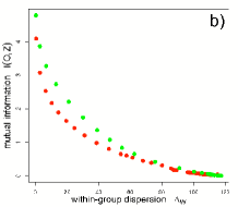
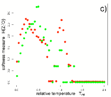
Figure 5: Comparison between the clustering obtained from $\hat{D}^{\mbox{\tiny\it sif}}$ (in red) and $\hat{D}^{\mbox{\tiny\it jump}}$ (in green): evolution of the number of effective clusters with the temperature (a), rate-distortion function (b) and overall softness measure (c). In (b), $\hat{\Delta}^{\mbox{\tiny\it jump}}$ has been multiplied by a factor five to fit to the scale.

5 Conclusion

Our first numerical results confirm the theoretical coherence and the tractability of the clustering procedure presented in this paper. Yet, further investigations are certainly required: in particular, the precise role that the diagonal components of the exchange matrix should play into the construction of distances on graphs deserves to be thoroughly elucidated. Also, the presence of fairly small clusters in the clustering solutions of Section 4, from which the normalized cut algorithm Ncut was supposed to prevent, should be fully understood. Our present guess is that small clusters are inherent to the spatial nature of the data under consideration: elongated and connected clouds as those of Figure 4 cannot miraculously split into well-distinct groups, irrespectively of the details of the clustering algorithm (classical chaining problem). This being said, squared Euclidean are closed under addition and convex mixtures. Hence, an elementary yet principled remedy could simply consist in adding spatial squared Euclidean distances to the flow-induced distances investigated in the present contribution.

References

- [1]
- [2] Aldous, D. and Fill, J. Reversible Markov Chains and Random Walks on Graphs. Draft chapters, online version available at http://www.stat.berkeley.edu/users/aldous/RWG/book.html
- [3] Bavaud, F.: The quasi-symmetric side of gravity modelling. Environment and Planning A 34, 61–79 (2002)
- [4] Bavaud, F.: Spectral clustering and multidimensional scaling: a unified view. In: Data science and classification (Batagelj, V., Bock, H.-H., Ferligoj, A., and Ziberna, A. editors), 131–139 Springer (2006)
- [5] Bavaud, F.: The Endogenous analysis of flows, with applications to migrations, social mobility and opinion shifts. Journal of Mathematical Sociology 32, 239–266 (2008)
- [6] Bavaud, F.: Aggregation invariance in general clustering approaches. Advances in Data Analysis and Classification 3, 205–225 (2009)
- [7] Bavaud, F.: On the Schoenberg Transformations in Data Analysis: Theory and Illustrations. Submitted (2010)
- [8] Belkin, M., Niyogi, P.: Laplacian Eigenmaps for Dimensionality Reduction and Data Representation. Neural Computation 15, 1373–1396 (2003)
- [9] Berger, J., Snell, J.L.: On the concept of equal exchange. Behavioral Science 2, 111–118 (1957)
- [10] Beurling, A., Deny, J.: Espaces de Dirichlet. I. Le cas élémentaire. Acta Mathematica 99, 203–224 (1958)
- [11] Chung, F.R.K.: Spectral graph theory. CBMS Regional Conference Series in Mathematics 92. American Mathematical Society, Washington (1997)
- [12] Cover, T. M., Thomas, J. A. Elements of Information Theory. Wiley (1991)
- [13] Critchley, F., Fichet, B. The partial order by inclusion of the principal classes of dissimilarity on a finite set, and some of their basic properties. In: Classification and dissimilarity analysis (van Cutsem, B., ed.). Lecture Notes in Statistics. Springer. 5–65 (1994)
- [14] Deza, M., Laurent, M.: Geometry of cuts and metrics. Springer (1997)
- [15] Dunn, G., Everitt, B.: An Introduction to Mathematical Taxonomy. Cambridge University Press (1982)
- [16] Filippone, M., Camastra, F., Masulli, F., Rovetta, S.: A survey of kernel and spectral methods for clustering. Pattern Recognition 41, 176–190 (2008)
- [17] Fouss, F., Pirotte, A., Renders, J.-M., Saerens, M.: Random-walk computation of similarities between nodes of a graph with application to collaborative recommendation. IEEE Transactions on Knowledge and Data Engineering 19, 355–369 (2007)
- [18] Greenacre, M., J.: Correspondence analysis in practice. Chapman & Hall (2007)
- [19] Hein, M., Bousquet, O., Schölkopf, B.: Maximal margin classification for metric spaces. Journal of Computer and System Sciences 71, 333–359 (2005)
- [20] Huang, Z., Ng, M.K.: A fuzzy k-modes algorithm for clustering categorical data. IEEE Transactions on Fuzzy Systems 7, 446–452 (1999)
- [21] Kemeny, J.G., Snell, J.L.: Finite Markov Chains. Springer (1976)
- [22] Kijima, M.: Markov processes for stochastic modeling. Chapman & Hall (1997)
- [23] Kondor, R.I., Lafferty, J.D.: Diffusion kernels on graphs and other discrete input spaces. In: Proceedings of the Nineteenth International Conference on Machine Learning (Sammut, C., Hoffmann, A.G., editors) 315–322 (2002)
- [24] Lafon, S., Lee, A.B. : Diffusion Maps and Coarse-Graining: A Unified Framework for Dimensionality Reduction, Graph Partitioning, and Data Set Parameterization. IEEE Trans. on Pattern Analysis and Machine Intelligence 28, 1393–1403 (2006)
- [25] von Luxburg, U.,: A tutorial on spectral clustering. Statistics and Computing 17, 395–416 (2007)
- [26] Mardia, K.V., Kent, J.T., Bibby, J. M.: Multivariate analysis. Academic Press (1979)
- [27] Meila, M.: Comparing clusterings: an axiomatic view. ACM International Conference Proceeding Series 119, 577–584 (2005)
- [28] Ng, A., Jordan, M., Weiss, Y.: On spectral clustering: analysis and an algorithm. In: Advances in Neural Information Processing Systems 14, 849–856. MIT Press (2002)
- [29] Nock, R., Vaillant, P., Henry, C., Nielsen, F.: Soft memberships for spectral clustering, with application to permeable language distinction. Pattern Recognition 42, 43–53 (2009)
- [30] Rose, K., Gurewitz, E., Fox, G. C.,: Statistical mechanics and phase transitions in clustering. Phys. Rev. Lett. 65, 945–948 (1990)
- [31] Rose, K.: Deterministic Annealing for clustering, compression, classification, regression, and related optimization problems. Proceedings of the IEEE 86, 2210–2239 (1998)
- [32] Schoenberg, I. J.: Metric Spaces and Completely Monotone Functions. The Annals of Mathematics 39, 811–841 (1938a)
- [33] Schoenberg, I. J.: Metric Spaces and Positive Definite Functions. Transactions of the American Mathematical Society 44, 522–536 (1938b)
- [34] Schölkopf, B.: The Kernel Trick for Distances. In: Advances in Neural Information Processing Systems 13, 301–307 (2000)
- [35] Shi, J., Malik, J. Normalized cuts and image segmentation. IEEE Transactions on Pattern Analysis and Machine Intelligence 22, 888–905 (2000)
- [36] Tenenbaum, J.B., de Silva, V., Langford, J.C.: A Global Geometric Framework for Nonlinear Dimensionality Reduction. Science 22, 2319–2323 (2000)
- [37] Torgerson, W.S. Theory and Methods of Scaling, Wiley (1958)
- [38] Williams, C.K.I., On a Connection between Kernel PCA and Metric Multidimensional Scaling. Machine Learning 46, 11–19 (2002)
- [39] Young, G., Householder, A. S.: Discussion of a set of points in terms of their mutual distances. Psychometrika 3, 19–22 (1938)
- [40] Yu, S.X., Shi., Multiclass Spectral Clustering. Proceedings of the Ninth IEEE International Conference on Computer Vision, 313–319 (2003)