Colours of Bulges and Discs within Galaxy Clusters and the Signature of Disc Fading on Infall

Abstract

The origins of the bulge and disc components of galaxies are of primary importance to understanding galaxy formation. Here bulge-disc decomposition is performed simultaneously in $B$- and $R$-bands for 922 bright galaxies in 8 nearby $(z<0.06$) clusters with deep redshift coverage using photometry from the NOAO Fundamental Plane Survey. The total galaxy colours follow a universal colour-magnitude relation (CMR).

The discs of $L_{*}$ galaxies are $0.24$ magnitudes bluer in $B-R$ than bulges. Bulges have a significant CMR slope while the CMR slope of discs is flat.

Thus the slope of the CMR of the total light is driven primarily (60%) by the bulge-CMR, and to a lesser extent (40%) by the change in the bulge-to-total ratio as a function of magnitude. The colours of the bulge and disc components do not depend on the bulge-to-total ratio, for galaxies with bulge-to-total ratios greater than 0.2. While the colours of the bulge components do not depend significantly on environment, the median colours of discs vary significantly, with discs in the cluster centre redder by 0.10 magnitudes than those at the virial radius. Thus while star formation in bulges appears to be regulated primarily by mass-dependent, and hence presumably internal, processes, that of discs is affected by the cluster environment.

1 Introduction

It is well-known that, at low redshifts, the centres of galaxy clusters are dominated by red, early-type galaxies. The morphology-density relation dates back to Hubble & Humason (1931), and was more accurately quantified by Dressler (1980) and Postman & Geller (1984). The early-type galaxies (ellipticals and S0s) follow tight scaling relations, such as the Fundamental Plane (Dressler et al., 1987; Djorgovski & Davis, 1987) and the colour-magnitude relation (hereafter CMR, Sandage & Visvanathan, 1978; Bower et al., 1992). Indeed it is the existence of a tight CMR for red galaxies that allows one to isolate a “red-sequence” population.

The dependence of the red-sequence CMR on environment is weak (Sandage & Visvanathan, 1978), but real (Abraham et al., 1996; van Dokkum et al., 1998; Balogh et al., 2000; Carter et al., 2002; López-Cruz et al., 2004; Balogh et al., 2004; Hogg et al., 2004; Barazza et al., 2009) although in detail the strength of the effect depends on the morphological selection and on the magnitude range of the sample. These studies are based on global galaxy colours, from which it is impossible to disentangle whether such trends might be due to, for example, the colour of the bulge, the colour of the disc, or the varying relative importance of bulge and disc components.

Recent spectroscopic studies of the centres of red-sequence giant galaxies have shown that, at a given mass, those in the cores of rich clusters are slightly older (by a few Gyr at most) than their counterparts in lower-density environments, such as the outskirts of clusters (Smith et al., 2006), groups (Proctor et al., 2004) or the field (Thomas et al., 2005; Bernardi et al., 2006). There is little evidence of an environmental dependence of metallicity (at fixed mass), although the results of Smith et al. (2006) suggest that giant ($\sim L_{*}$) red galaxies on the outskirts of clusters are $\sim 15\%$ younger and less enhanced in $\alpha$-elements than those in the cluster cores. For fainter dwarf galaxies ($M_{r}\mathrel{\hbox{\hbox to0.0pt{\hbox{\lower 4.0pt\hbox{$\sim$}}\hss}\hbox{$>$}}}-17.5$), the environmental dependence is stronger: Smith et al. (2008b, 2009b) have shown that the stellar ages of dwarf red-sequence galaxies in Coma vary by a factor $\sim 3$ from the core to the virial radius.

Spiral galaxies in clusters, when compared to their counterparts in the field, are redder (Holmberg, 1958; Kennicutt, 1983; Bamford et al., 2009) and “anaemic” in appearance (van den Bergh, 1976; McIntosh et al., 2004), and poorer in neutral hydrogen (Davies & Lewis, 1973; Sullivan et al., 1981; Haynes et al., 1984; Giovanelli & Haynes, 1985; Cayatte et al., 1990).Several mechanisms have been proposed for the dependence of spiral galaxy properties on environment: ram-pressure stripping of the cold gas (Gunn & Gott, 1972), the removal of the hot gas halo (Larson et al., 1980), sometimes known as “strangulation” (Balogh & Morris, 2000) and tidal stripping by the cluster potential (Merritt, 1984; Mamon, 1987) or by encounters with other galaxies (Gallagher & Ostriker, 1972; Moore et al., 1998). The former mechanisms remove the gas that is the fuel for star formation, and so the stellar disc will dim and redden as its stars age. This will obviously affect the colour of the disc as well as the $B/T$ ratio. In the tidal stripping scenario, outer parts of the stellar and gaseous discs are removed. A recent review of the effects of such processes on late-type galaxies in clusters is given by Boselli & Gavazzi (2006).

From observations at higher redshifts, it is known that, in the past, clusters contained a higher proportion of spirals compared to S0s (Dressler et al., 1997; Fasano et al., 2000) than present-day clusters. van Dokkum et al. (1998) have shown that S0s are bluer and have a larger scatter in colour than ellipticals in a $z\sim 0.3$ cluster, suggesting that some of them may have recently arrived on the red sequence.

Clearly it is of interest to study the colours of bulge and disc components separately, since the separate components likely have different stellar ages and metallicities, and will be affected differently by environmental processes. Most previous studies have focused on the global colours of galaxies (sometimes subdivided by morphological class). Since most galaxies have both a bulge and a disc component, this global approach makes it difficult to disentangle the effects of the two components. There have been few previous studies in which the separate colours of bulge and disc components have been analyzed. In the field, Balcells & Peletier (1994); Terndrup et al. (1994); Peletier & Balcells (1996); MacArthur et al. (2004), among others, have studied colours of disc and bulge components in spirals and S0s. In clusters, two-dimensional decompositions have been performed (Caon et al., 1990; D’Onofrio, 2001; Gutiérrez et al., 2004; Christlein & Zabludoff, 2004; de Jong et al., 2004), but the only paper to perform this decomposition in multiple bands simultaneously is Koo et al. (2005), who studied the $z\sim 0.83$ cluster MS 1054-03.

The goals of this paper are twofold. The first goal is to determine the origin of the slope of the red-sequence CMR by decomposing cluster galaxies into their constituent bulge and disc components, and studying the colours of each component separately. The second goal is to determine how environment affects each of these components separately, as well as how it affects the global morphology, quantified by the bulge-to-total ratio (hereafter $B/T$). Other structural parameters (bulge effective radii and surface brightnesses, Sérsic indices and disc central surface brightness and scale lengths) will be examined in future work.

The outline of the paper is as follows. Section 2 describes the sample of cluster galaxies, and details of the photometric and redshift data. Section 3 describes the morphologies and bulge-to-total ratios. In Section 4, the total-light CMR, as well as the CMRs for bulge and disc components is measured and its physical interpretation is discussed in Section 5. Section 6 quantifies the environmental dependence of the CMRs and the astrophysical implications are discussed in Section 7 . Throughout we adopt a Hubble parameter, $h=H_{0}/(100\>\mbox{\rm km~{}s\mbox{${}^{-1}$}}\>\mbox{\rm Mpc}^{-1})=1$ and a $\Omega_{\rm m}=0.3$, $\Omega_{\Lambda}=0.7$ cosmology.

2 Data

2.1 Cluster Sample

As noted above, the goals of this paper are to determine the physical origin of the colour-magnitude relation and its environmental dependence within clusters. In particular, we are interested not only in the dominant red-sequence galaxies but also the contribution of blue galaxies. Photometry for the $\sim 90$ most luminous nearby clusters has been obtained as part of the NOAO Fundamental Plane Survey (hereafter NFPS). The spectroscopic component of the NFPS (Smith et al., 2004) was, however, designed to follow-up only the red galaxies. In this paper, therefore, we focus on NFPS clusters with complete photometry for which nearly complete deep redshift samples are available from the literature. Eight NFPS clusters previously studied by ENACS (Katgert et al., 1998), by Christlein & Zabludoff (2003), by the CAIRNS project (Rines et al., 2003) and in the SDSS DR2 (Abazajian et al., 2004) were selected, and are listed in Table 1. The typical cluster in our sample has a redshift of 14 800 km s^-1, a velocity dispersion, $\sigma_{\rm cl}$ of 860 km s^-1, and a virial ($r_{200}$) radius of 1.46 $h\mbox{${}^{-1}$}$Mpc, where $r_{200}=\sqrt{3}\,(\sigma_{\rm cl}/1000\>\mbox{\rm km~{}s\mbox{${}^{-1}$}})\,\mbox{$h\mbox{${}^{-1}$}$}\>\mbox{\rm Mpc}$ (Carlberg et al., 1997). The data extend to the virial radius, $r_{200}$, and are complete within $r_{200}/2$. Galaxies are assumed to be cluster members if their velocities lie within $\pm 3\sigma_{\rm cl}$ of the cluster mean. Details of the galaxy completeness as a function of magnitude and colour will be discussed in Section 2.4.

2.2 Field Sample

In Section 6, we will also compare properties of cluster galaxies to those in the field. In the foreground and background of the eight clusters, there are 35 field galaxies (after exclusion of two background clusters behind A0085 and A0151). The median $R-$band magnitude of the field sample is $-20.3$, very similar to that of the cluster sample. These field data are analyzed in exactly the same way as the cluster sample described above.

Table 1: Cluster Sample. $N_{z}$ is the number of galaxies with $M_{R}<-19.5$. Phot is the source of photometry: K=KPNO; C=CTIO.

Cluster	R.A.	Decl.	$<cz>$	$N_{z}$	$M_{\rm lim}$	$\sigma_{\rm cl}$	$r_{200}$	Phot
	(J2000)	(J2000)	km s-1			km s-1	$h\mbox{${}^{-1}$}$Mpc
A0085	00 41 50.4	–09 18 11	16392	144	–18.0	905	1.57	K
A0119	00 56 16.1	–01 15 18	12958	80	–19.5	747	1.29	K
A0151	01 08 51.8	–15 25 12	15769	51	–19.5	838	1.45	K,C
A3128	03 30 23.5	–52 32 24	17934	107	–19.5	849	1.47	C
A3158	03 42 56.6	–53 38 02	17542	88	–19.5	954	1.65	C
A0496	04 33 37.7	–13 15 43	9717	127	–18.0	722	1.25	K
A0576	07 21 24.2	+55 47 02	11527	60	–19.5	871	1.51	K
A3667	20 13 33.4	–56 50 35	16585	93	–19.5	1000	1.73	C

2.3 Photometric Data

The photometric data used were obtained as part of the NFPS (Smith et al., 2004), from the Kitt Peak National Observatory (KPNO) 0.9 meter and the Cerro Tololo Inter-American Observatory (CTIO) 4.0 meter telescopes. The fields of view were $59^{\prime}$ x $59^{\prime}$ and $37^{\prime}$ x $37^{\prime}$ for KPNO and CTIO, respectively, and were centreed on the nominal X-ray centroid of the cluster. Exposure times were typically 400 ($R$) and 600 ($B$) seconds at KPNO, and 60 ($R$) and 150 ($B$) seconds at CTIO. The seeing point spread function (PSF) full-width at half maximum typically was $\sim 1.5$ arcseconds for KPNO and $\sim 1.1$ arcseconds for CTIO.

Data were reduced with the IRAF mscred package, and were calibrated to the Johnson-Cousins $BR$ system using Landolt (1992) standard stars. Objects and masks were generated with SExtractor (Bertin & Arnouts, 1996).

2.4 Corrections and Completeness

Redshifts of galaxies within our images were gathered from the NFPS spectroscopic survey (Smith et al., 2004) and from the NASA Extragalactic Database (NED). Galaxies were assigned cluster membership using an iterative $3\sigma$-clipping technique. Apparent magnitudes were converted into absolute magnitudes using cluster redshift in the Cosmic Microwave Background (CMB) frame.

Galactic extinction corrections were applied using the $E(B-V)$ map of Schlegel et al. (1998, hereafter SFD), and converted to extinction using $4.325\,\mbox{$E(B-V)$}$ for the B band and $2.634\,\mbox{$E(B-V)$}$ for the $R$-band (SFD). K-corrections were applied to the bulge and disc components separately, by interpolating as a function of morphological type from the tables in Frei & Gunn (1994).

Fig. 1 shows that in general, the redshift data are complete at the bright end ($M_{R}\mathrel{\hbox{\hbox to0.0pt{\hbox{\lower 4.0pt\hbox{$\sim$}}\hss}\hbox{$<$}}}-20$), but that, as expected, the completeness decreases at fainter magnitudes. To measure the completeness, a Schechter luminosity function was fit to each cluster with galaxies with $M_{R}<-21$ fixing $M^{*}_{R}=-21.14$ and $\alpha=-1.21$ (Christlein & Zabludoff, 2003), but leaving the normalization, $\phi_{*}$, free. The fit is shown by the dotted line in Fig. 1.

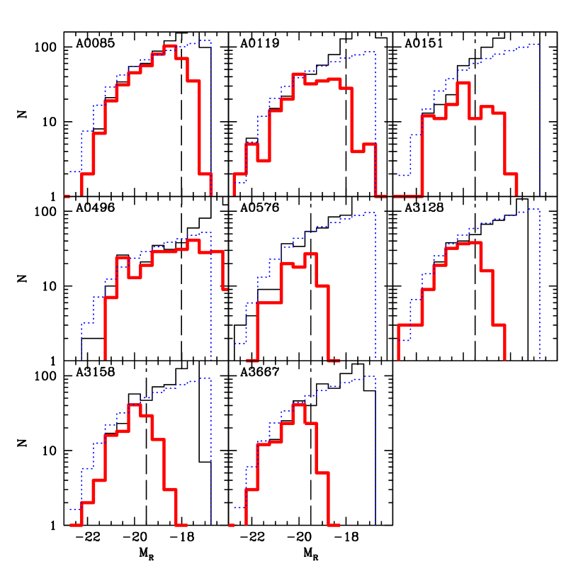
Figure 1: $R$-band magnitude histograms for individual clusters. The thin black histogram is all galaxies with photometry, whereas the thick red histogram shows those with published redshifts. The luminosity functions (normalized at the bright end by assuming a Schechter function) are shown by the blue dotted line. In each panel, the vertical dashed line indicates the absolute magnitude limit adopted for that cluster.

Based on Fig. 1, we adopt a Galactic-extinction-corrected absolute magnitude limit of $M_{R}<-19.5$ for our primary sample. For the sample as a whole, the average completeness brighter this limiting magnitude is 87%, and the completeness in the faintest 0.5 mag bin is 66%. To correct for incompleteness, galaxies with redshifts are assigned a weight that is the inverse of the probability that a cluster member of that magnitude has a measured redshift. Note that the clusters A0085, A0119 and A0496 have redshift data that are considerably deeper. These three clusters are used to define a deeper $M_{R}<-18$ sample, which will be used later to assess correlations at fainter magnitudes.

2.5 GIM2D Morphological Parameters

Bulge and disc decomposition is based on the GIM2D morphology package (Simard et al., 2002) which analyses postage-stamp images along with bad-pixel masks, PSF images, and error maps and fits a PSF-convolved model galaxy to the two-dimensional images. The GIM2D model consists of a infinitesimally-thin exponential disc and an axisymmetric Sérsic bulge. The fit yields bulge and disc magnitudes, radii, position angles, and inclinations (for discs), or ellipticities and Sérsic index $n$ (for the bulge components).

Note that we could have chosen to fit the $B$ and $R$-band images independently, but in that case, it would have been possible to obtain different values in the two bands for parameters such as the radii and position angles of given component. In particular, because of, for example, systematic errors in the PSF, there can be a trade-off between the flux in the bulge and the flux in the disc components. If such systematic errors were different in the two bands, the colours of the bulge and disc components would not be robust. Instead, we used GIM2D in the two-band mode, in which simultaneous fits to the two images are made for the radii, position angles, bulge Sérsic index $n$, bulge ellipticity and disc inclination, while bulge and disc fluxes are free in each filter over all pixels in the SExtractor (Bertin & Arnouts, 1996) segmentation mask. While errors of the type described above can still affect these fits, in general, one would expect them to be yield more robust colours for the individual components.

A limitation of two-band mode is that the bulge effective radii are assumed to be the same in both $B$ and $R$ bands, and likewise for the disc scale lengths. In reality, disc scale lengths are likely to differ, although for the S0s and early-type spirals studied here the difference is quite small: Noordermeer & van der Hulst (2007) find that the disc scale lengths in a sample of S0-Sab galaxies are larger by $3.2\pm 2.5$% in the $B$-band than in the $R$-band. We have simulated the impact that this GIM2D fitting constraint may have on disc colours by fitting model galaxies with disc scale length assumed to be different from the true one. We find that for a 3% error in scale length, the colour is biased at a level of 0.01 mags. Thus this is a small effect.

2.6 Data Comparison

Before proceeding with the analysis of the data, a check was performed to ensure internal consistency of the photometric data and GIM2D decompositions. Of the clusters in the sample, only A0151 was observed both at KPNO and at CTIO. Figures 2 shows the comparison of the A0151 data obtained from the different observatories, in the sense $\Delta\equiv$ KPNO - CTIO. In the magnitude comparisons (top panels of Figure 2), the median offset is $0.007$ magnitudes in the $R$-band and $0.025$ magnitudes in the $B$-band.

The scatter is larger than the individual measurement errors quoted by GIM2D. This suggests that GIM2D errors are underestimated, which is expected since these reflect only the error due to photon noise, and not e.g. seeing mismatches, sky subtraction etc. Therefore, to the quoted GIM2D magnitude errors, we add in quadrature a magnitude-independent extra “systematic” error. Based on the scatter in the top panel of Fig. 2, we find that this extra error is 0.05 magnitudes.

The $B-R$ colour comparison is shown in the second panel of Figure 2. The median offset between KPNO and CTIO is $0.02$ magnitudes, which is acceptable for the purposes of this study. The measured scatter suggests that individual colour measurements are accurate to 0.03 magnitudes. This is smaller than the magnitude error in either band separately, and is due to the fact that the fit is made simultaneously in both bands. From similar comparisons (see bottom panels of Fig. 2), errors in a single measurement of the bulge and disc colours are estimated to be 0.07 and 0.11, respectively.

Figure 2: Comparison of the total magnitudes and colours as measured by GIM2D from independent runs. $\Delta$ is in the sense KPNO $-$ CTIO. The upper panel compare the $R$-band magnitudes, the second panel shows the global $B-R$ colour comparison, and the bottom two panels compare bulge and disc colours. The median offsets are small.

Figure 3 shows the differences in the bulge-to-total light ratios. The observed scatter in the R-band $B/T$ values is larger than the GIM2D errors. Therefore, we add in quadrature a systematic error of $0.07$ per individual $B/T$ measurement. Given the random (noise) errors, the total measurement error in $B/T$ is then typically $\sim 0.08$.

Figure 3: Difference between the $R$-band $B/T$ measured from CTIO and from KPNO as a function of average $R$-band $B/T$. The plotted GIM2D errors underestimate the differences, which presumably arise from other systematic sources of error such as modelling the PSF.

3 Morphologies and Bulge-to-Total Ratios

3.1 Visual Morphological Classification

For a subset of the sample described above, postage stamp images, pixel masks and GIM2D residual images for all galaxies were inspected visually by one of us (GAW) and a visual morphological classification was assigned to each galaxy. Furthermore, cases where the automated pixel masking had failed (e.g. close galaxy pairs or missed bad columns, etc) were flagged and rejected from the sample.

Fig. 4 compares the R-band bulge-to-total ($B/T$) ratios from GIM2D with the visual classification. The visual classifications were labeled according to the corresponding T-type and plotted against $B/T$. The trend of decreasing $B/T$ with increasing T-type, and the dispersion in $B/T$ ($\sim 0.17$) at a given type, are in generally in good agreement with previous studies (Kent, 1985; Simien & de Vaucouleurs, 1986), although the median $\mbox{$B/T$}\ \sim 0.3$ for Sc galaxies is somewhat higher than expected. Since the measurement error in $B/T$ is typically $0.08$ (Section 2.6), the intrinsic scatter in $B/T$ of a given T-type is $\sim 0.15$.

Figure 4: Visual morphological classifications encoded by $T$-type (de Vaucouleurs et al., 1991) versus R-band $B/T$. The filled circles show the mean $B/T$ at each $T$-type, and the long errorbars indicate the dispersion in $B/T$ at each type. The short errorbars are the error in the mean. Small dots are individual data points, with the $T$ slightly randomized for graphical purposes. The number of galaxies in each bin is also indicated.

3.2 Tests of the GIM2D decomposition

GIM2D fits a Sérsic bulge plus disc model to the $B-$ and $R-$band data simultaneously. While we argue above that the constraints of these fits lead to more robust colours of the bulge and disc components, it’s not necessarily true that these components — needed to reproduce the 2-D light distribution — correspond to real bulge and disc components. For example, a pure bulge component with an isophote twist might be fitted with a (untwisted) bulge and a “disc” which accommodates the twist.

One way to check the reality of the bulge and disc components is by plotting their ellipticity distributions. If the “discs” are really related to the bulge components, they would be expected to follow the ellipticity distribution of bulges, i.e. there should be few with $\epsilon=1-b/a>0.5$. Fig. 5 shows the ellipticity distribution for bulges and disc components. If the discs are infinitely thin, transparent and seen at random inclinations, then they would have a uniform distribution in $\epsilon$. The discs in Fig. 5 are very close to this scenario, although there is a deficit of very high $\epsilon>0.9$ discs. We attribute this to the finite vertical scale-height of discs: even seen edge-on, such discs will have $b/a>0$. Note that this result is different from that found by Driver et al. (2007) for discs in the field. In addition to the deficit of very high $\epsilon$ discs, they also find a deficit of moderately-inclined discs: for example, in the range $0.5\mathrel{\hbox{\hbox to0.0pt{\hbox{\lower 4.0pt\hbox{$\sim$}}\hss}\hbox{$<$}}}\epsilon\mathrel{\hbox{\hbox to0.0pt{\hbox{\lower 4.0pt\hbox{$\sim$}}\hss}\hbox{$<$}}}0.7$ (corresponding to $60\degr\mathrel{\hbox{\hbox to0.0pt{\hbox{\lower 4.0pt\hbox{$\sim$}}\hss}\hbox{$<$}}}i\mathrel{\hbox{\hbox to0.0pt{\hbox{\lower 4.0pt\hbox{$\sim$}}\hss}\hbox{$<$}}}73$) their counts are reduced by $\sim 40\%$ (cf. their Figure 5), whereas ours are consistent with being constant. They conclude that dust obscuration dims these moderately-inclined galaxies resulting in their under-representation in a magnitude-limited survey. In contrast, our uncorrected disc $\epsilon$ distribution looks very similar to their distribution after correction for dust extinction. The difference between the field and cluster disc ellipticities suggests that cluster discs may be depleted in dust, and hence considerably more transparent. In contrast to the flat distribution of disc ellipticities, the bulge components are clustered between $0.1<\epsilon<0.5$, as expected based on the distribution of E+S0 ellipticities in clusters (e.g. Jorgensen & Franx, 1994).

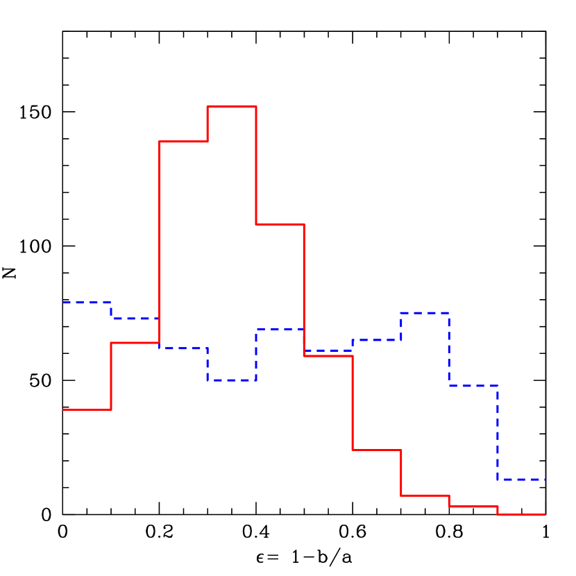
Figure 5: Distribution of ellipticity for disc (dashed blue) and bulge (solid red) components. Note that there is not an excess of disc components with ellipticities typical of bulges. The two distributions are very close to what one expects a priori on physical grounds indicating that the disc and bulge components are not artifacts of the fitting procedure.

3.3 Dependence of $B/T$ on Magnitude and Environment

Before discussing the colours of bulge and disc components, it is interesting to study the dependence of $B/T$ on magnitude and environment. Throughout this paper, unless explicitly stated otherwise,$B/T$ refers to the $R$-band value. Fig. 6 shows the weak, but statistically significant, dependence of the bulge-to-total ratio on magnitude, with more luminous galaxies being more bulge-dominated, mirroring the trend of morphological type with luminosity.

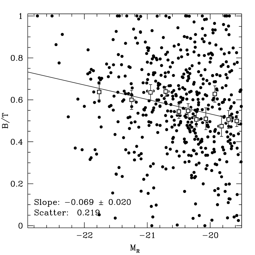
Figure 6: $B/T$ in the $R$-band as a function of magnitude for the $M_{R}<-19.5$ sample. The square symbols with error bars show the median $B/T$ in a bins of magnitude. The solid line is a fit to the medians.

The morphology-radius relation, where morphology is quantified by $B/T$ and the projected radius, $r_{p}$ is scaled by the virial radius, $r_{200}$, is shown in Fig. 7. The variation in $B/T$ is rather weak: only in the very innermost regions ($\mbox{$r_{\rm p}$}\mathrel{\hbox{\hbox to0.0pt{\hbox{\lower 4.0pt\hbox{$\sim$}}\hss}\hbox{$<$}}}0.2\,r_{200}$) is there evidence for a difference in the median $B/T$. However, a Spearmank rank correlation test does suggest a correlation at the 98.7% confidence level. Moreover, fitting $B/T$ as a function of $\log(\mbox{$r_{\rm p}$}/r_{200})$ yields a significant slope: $-0.108\pm 0.033$. Thus while there is a clear difference between morphologies in clusters and in the field, the morphological segregation as defined by $B/T$ within clusters appears to be limited to the innermost regions.

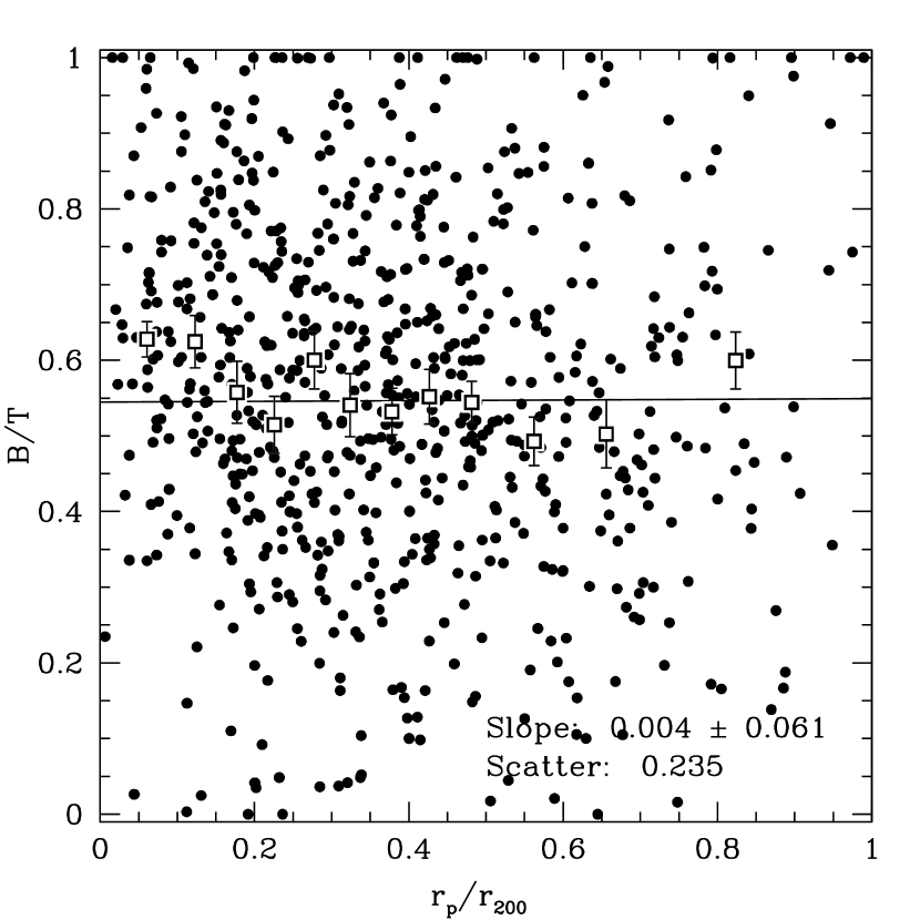
Figure 7: $B/T$ in the $R$-band as a function of scaled projected radius for the $M_{R}<-19.5$ sample. The square symbols with error bars show the median $B/T$ in a bin of $\mbox{$r_{\rm p}$}/r_{200}$. The line is a fit to the medians.

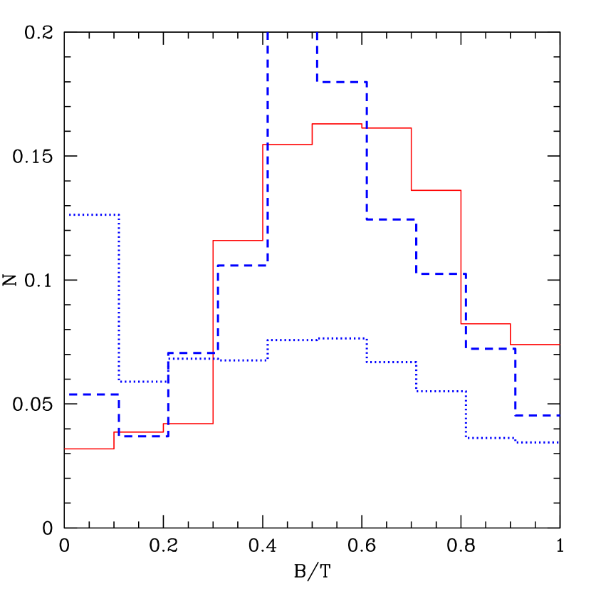
Figure 8: The solid red histogram shows the distribution of $R-$band $B/T$ for $M_{R}<-19.5$ galaxies in the NFPS clusters, the dashed blue line is the same but for the $B-$band $B/T$, and, for comparison, the dotted blue line shows the $B-$band $B/T$ for the field sample (Allen et al., 2006), selected to the same magnitude limit as the cluster sample ($M_{R}<-19.5$). The most striking differences are the excess of late-type spiral ($\mbox{$B/T$}<0.1$) systems in the field, and the excess of S0-like ($0.4<\mbox{$B/T$}\ <0.6$) morphologies in the cluster.

Finally, it is interesting to compare the cluster results with those in the field. The distribution of $B/T$ (for $\mbox{$r_{\rm p}$}<0.5\,r_{200}$) is shown in Fig. 8. For comparison, we also show the $B-$ band $B/T$ distribution in the field (Allen et al., 2006) for the same absolute magnitude limit as applied to the NFPS clusters. Compared to the field, clusters contain an excess of galaxies with S0 morphology ($0.4<\mbox{$B/T$}<0.6$), and a clear deficit of spirals, particularly those of the latest types, or lowest bulge fractions $(\mbox{$B/T$}<0.1)$. The distribution of $B/T$ in the group environment (McGee et al., 2008) is intermediate between that in the field and in clusters.

4 The Red-Sequence Colour-Magnitude Relation Revisited

In this section we examine the global-colour vs. magnitude relation for individual clusters as well as the universal relation for all clusters. We then decompose the global-CMR into the CMRs for bulges and discs separately.

4.1 Robust Fits to Galaxies within $r_{200}/2$

We will show below (Section 6) that the colours of some components depend on cluster-centric radius. Consequently, in this section, we restrict fits to galaxies with projected cluster-centric radii $\mbox{$r_{\rm p}$}<r_{200}/2$. Furthermore for fits to the red-sequence, we do not wish to be biased by very blue galaxies, nor by outliers with anomalous colours. Therefore, in order to fit the CMR in a robust way, the data were first binned by magnitude, with an equal number of data points in each bin. For each bin the median was calculated, and a linear least squares trend was fit to these medians.

To estimate the scatter of the data, the semi-interquartile range (SIQR) of the data is calculated, which is then converted into a the equivalent dispersion ($\sigma=1.5\mathrm{SIQR}$) of a Gaussian with the same SIQR. In order to compare the colour-magnitude relations with different slopes, a normalized colour is defined, $(B-R)_{*}$ the value of the fit at $M^{*}_{R}=-21.14$. The errors on the normalized colour were calculated using 1000 bootstraps.

4.2 Global Colour-Magnitude Relation

The global colour-magnitude relation is shown in Figure 9. For galaxies with $M_{R}<-19.5$ the normalized colour at $M^{*}_{R}$ is $(B-R)_{*}=1.485\pm 0.009$ magnitudes, with a CMR slope of $-0.031\pm 0.006$. For the fainter subsample of A0085, A0119 and A0496 combined, which extends to $R<-18.0$, the slope steepens slightly to $-0.042\pm 0.007$ with the normalized colour being $1.463\pm 0.012$. Note that López-Cruz et al. (2004) find a CMR slope of $-0.052\pm 0.008$ for $M_{R}\leq-18.6$, which is consistent with our result within the uncertainties.

The “1-sigma” scatter in the colour-relation is $0.07$ magnitudes, as estimated via the SIQR. Note that the measurement error in $B-R$ is estimated to be $0.03$, so this yields a intrinsic scatter of $0.06$. This is consistent with the value ($0.074$) found by López-Cruz et al. (2004), although their limiting magnitude ($M_{R}=-18.6$) is somewhat fainter whereas their radial limit ($0.2\,r_{200}$) is smaller than ours ($0.5\,r_{200}$).

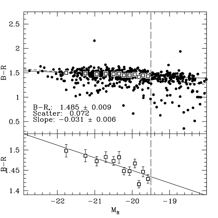
Figure 9: The colour-magnitude diagram for all 8 clusters combined. Upper panel: Filled circles indicate total-light colours of individual cluster galaxies with $\mbox{$r_{\rm p}$}<0.5r_{200}$. Median colours in bins of magnitude are shown by the open squares. The robust fit to the median colours is shown by the solid line is to galaxies with $M_{R}<-19.5$ and $\mbox{$r_{\rm p}$}<r_{200}/2$. Lower panel: Same median data as in the upper panel, but shown at a different scale to better see the slope.

4.3 Fraction of Blue Galaxies

The blue fraction was defined by Butcher & Oemler (1984, hereafter BO) to be the fraction of galaxies brighter than $M_{V}=-20$, lying within a third of the cluster radius and bluer than the red sequence by 0.2 mags in $B-V$. After correcting for cosmology, we find that their magnitude corresponds to $M_{R}=-19.1$, which is only $0.4$ mags fainter than our completeness limit. To match the BO definition as closely as possible, here we define a blue galaxy is as one with $(B-R)<1.25$ after having normalized to $M_{*}$ by correcting for the CMR slope, i.e. 0.24 magnitudes bluer than the red sequence. Within $0.5\,r_{200}$ there are only 35 blue galaxies of 595 in total in the 8 clusters, yielding a blue fraction of $5.9\pm 1.0$%. For A0085, A0119 and A046, the clusters complete to $M_{R}<-18$, within $0.5\,r_{200}$, the blue fraction climbs from $12/183$ ($6.5\pm 1.9\%$) at $M_{R}<-19.5$ to $27/259=10.4\pm 2.0$% at $M_{R}<-19$. This suggests that the blue fraction for the whole sample to $M_{R}<-19$ is $10\pm 2\%$. This blue fraction is considerably less than the blue fractions ($\sim$25%) at the same radius quoted in Andreon et al. (2006) for clusters at $z\sim 0.35$.

4.4 Colour-Magnitude Relations for Individual Clusters

The individual cluster colour-magnitude relations are shown in Figure 10. The normalized colours $(B-R)_{*}$ for each cluster are consistent with the global value. Only the slope in A0085 deviates by more than $2\sigma$ from the global slope. Thus there is no evidence for deviation from the universal CMR in our sample.

Figure 10: The colour-magnitude diagrams for each of the clusters. The solid line indicates the least-squares fit for the data in the cluster, and the dashed line shows global colour-magnitude relation. The fits are to the $M_{R}<-19.5$ sample.

4.5 Bulge and Disc Colour-Magnitude Relations

Having established that the total colours are uniform and consistent with previous results, we now turn to the main goal of this paper.

Our two-band GIM2D fits yield the colours and CMRs of the bulge and disc components separately. However, galaxies with very low $B/T$ do not have reliable bulge colours, so, in measuring the bulge colour-magnitude relation, we have omitted galaxies with $\mbox{$B/T$}<0.2$. This culled bulge colour-magnitude diagram is shown in the left panel of Figure 11. Note that the horizontal axis is the total $R-$band magnitude. The slope of the bulge CMR, $-0.037\pm 0.014$, is very similar to the slope of total-light CMR, however the normalized colour, $1.581\pm 0.091$, is 0.1 magnitudes redder than the total colour. Using the population synthesis models of Maraston, for an assumed metallicity $[Z/Z_{\hbox{$\odot$}}]=0.3$ dex, this colour corresponds to an SSP age of 12 Gyr. At fainter mags $M_{R}<-18$ the bulge CMR steepens to $-0.067\pm 0.017$.

The measured scatter in the bulge CMR ($0.093$) is actually somewhat larger than the total CMR scatter ($0.07$). This can be understood if one allows for additional error in the bulge-disc decomposition itself: some disc light is incorrectly assigned to the bulge and vice versa. In Section 2, we estimated from repeat measurements that the measurement error on the bulge colour is $\sim 0.07$, and so the intrinsic scatter is likely to be much lower.

If we fit bulge colour as a function of bulge magnitude, we obtain a flatter slope $-0.025\pm 0.013$, and larger scatter (0.098).However, in Section 5 we will show that bulge colour is most closely linked not to total magnitude but rather to central velocity dispersion.

Figure 11: (Left Panel) Bulge colour vs. total $R$-band magnitude. All galaxies which are disc-dominated $(\mbox{$B/T$}<0.2)$ have been removed. Symbols are as in Fig. 10. The solid line is the robust fit to bulge colours with $\mbox{$r_{\rm p}$}<r_{200}/2$ and $M_{R}<-19.5$. The dashed line is the total-colour-magnitude relation for comparison. (Right) Disc colour vs. total $R$-band magnitude. All galaxies which are bulge dominated $(\mbox{$B/T$}>0.8)$ have been removed for this comparison. Symbols and curves are as in the left panel.

The disc colour-magnitude relation for galaxies with $\mbox{$B/T$}<0.8$ is shown in the left panel of Figure 11. We find that discs have a flat CMR: the measured slope is $0.000\pm 0.010$. The disc colour for an $L_{*}$ galaxy ($1.353\pm 0.016$) is significantly bluer than that of the bulge component at the same total magnitude. Thus, in clusters, discs are bluer than bulges by $0.228\pm 0.024$ mags at $L_{*}$. The bulge-disc colour difference is larger than, but marginally consistent with, that found by Peletier & Balcells (1996) for S0-Sbc galaxies in the field ($0.045\pm 0.097$). On the other hand, the colour difference in clusters is smaller than the value $0.301\pm 0.014$ for a S0/a-Sdm field sample (MacArthur et al., 2004). At fainter magnitudes, the difference in colour is much less: at $M_{R}=-18$, $\sim 0.09\pm 0.06$ mags. The colour-magnitude relations are summarized in Table LABEL:tab:colmag. When disc colours are regressed against disc magnitude the slope is slightly negative, although the difference from zero is not statistically significant: $-0.006\pm 0.015$, and the scatter is similar ($0.120$) to the scatter versus total magnitude..

It is important to investigate whether bulge and disc colours depend on morphology. For example, in the field, MacArthur et al. (2004) found that the colours of both bulges and discs are correlated with morphology in the sense that later morphological types host both blue bulges and blue discs. Figure 12 shows a histogram of the bulge and disc colours for different bins of bulge-to-total ratio. The bulge and disc colours show no significant dependence on morphology for $\mbox{$B/T$}>0.2$. Discs in $\mbox{$B/T$}<0.2$ galaxies are significantly bluer than the discs in higher $B/T$ galaxies. However, there are few ($9\%$) such low $B/T$ galaxies in our sample.

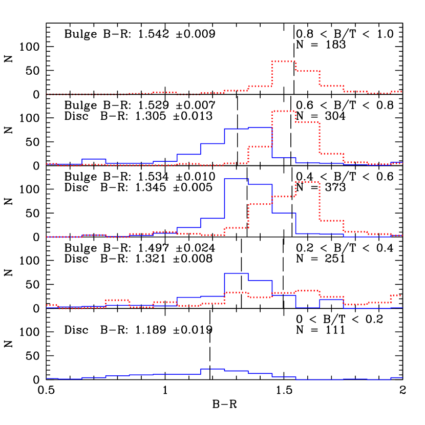
Figure 12: Histograms of the colours of disc (solid lines, for galaxies with $\mbox{$B/T$}<0.8$) and bulge (dotted lines, for galaxies with $\mbox{$B/T$}>0.2$) colours, for subsamples with different $B/T$. Note there is little dependence of disc or bulge colour on $B/T$, except for discs in very late types ($\mbox{$B/T$}<0.2$).

Table 2: Galaxy colours and properties as a function of magnitude.

Property	Mag Limit.	slope		value at $L_{*}$
Total Colour	$M<-19.5$	$-0.031$$\pm$	$0.006$	$1.485$$\pm$	$0.009$
Bulge Colour	$M<-19.5$	$-0.037$$\pm$	$0.014$	$1.581$$\pm$	$0.009$
Disc Colour	$M<-19.5$	$0.000$$\pm$	$0.010$	$1.353$$\pm$	$0.016$
$B/T$	$M<-19.5$	$-0.069$$\pm$	$0.020$	$0.614$$\pm$	$0.020$
Total Colour	$M<-18$	$-0.042$$\pm$	$0.007$	$1.463$$\pm$	$0.010$
Bulge Colour	$M<-18$	$-0.067$$\pm$	$0.017$	$1.596$$\pm$	$0.016$
Disc Colour	$M<-18$	$0.000$$\pm$	$0.014$	$1.307$$\pm$	$0.029$
$B/T$	$M<-18$	$-0.069$$\pm$	$0.019$	$0.643$$\pm$	$0.026$

4.6 Deconstructing the Colour-Magnitude Relation: Contributions from Bulge and Disc colours and from the Bulge-to-Total ratio

From the bulge and disc colour magnitude diagrams, it appears that the global CMR slope is due primarily to the colour of the bulge component. A quantitative check of this conclusion can be performed by reconstructing the global slope using the bulge and disc CMRs and the dependence of $B/T$-ratio on magnitude. Specifically, the global colour-magnitude relation can be decomposed as

$$\begin{split}\frac{\mbox{d}(B-R)}{\mbox{d}M_{R}}&=\frac{\partial\mbox{$B/T$}}{\partial M_{R}}[\mbox{$\left\langle B-R\right\rangle$}_{B}-\mbox{$\left\langle B-R\right\rangle$}_{D}]\\ &+\frac{\partial(B-R)_{B}}{\partial M_{R}}\mbox{$\left\langle\mbox{$B/T$}\right\rangle$}\\ &+\frac{\partial(B-R)_{D}}{\partial M_{R}}(1-\mbox{$\left\langle\mbox{$B/T$}\right\rangle$})\end{split}$$

For our $M_{R}<-19.5$ sample we measure an average $\mbox{$\left\langle B/T\right\rangle$}=0.566\pm 0.04$ and an average difference in bulge and disc colour is $\mbox{$\left\langle B-R\right\rangle$}_{B}-\mbox{$\left\langle B-R\right\rangle$}_{D}=0.237\pm 0.013$. Inserting the measured slopes from Table LABEL:tab:colmag and evaluating each term yields $-0.014\pm 0.004$ for the first ($B/T$) term, $-0.021\pm 0.008$ for the second (bulge CMR) term and zero from the third (disc CMR) term.

Thus the origin of the “tilt” or slope of the total-light-CMR is due mostly (60%) to the slope of bulge CMR, with the remainder of the total-light-CMR slope arising from the change in $B/T$ as a function of magnitude, which mixes in increasing more bluer disc light at fainter magnitudes. These trends, however, do not give insight into the ages or metallicities of the stellar populations of our sample. We address this topic in Section 5 below.

5 Discussion: The Origin of the CMR

We have shown that the tilt of the CMR is due primarily to the bulge CMR, and to a lesser extent, to the change in morphology along the red-sequence. The bulge-CMR itself has been thought to be due to an age-luminosity relation, a metallicity-luminosity relation, or both. While optical colours alone cannot break the “age-metallicity” degeneracy, in principle it is possible to do so by studying spectroscopic absorption linestrengths. Smith et al. (2009a) and Graves et al. (2009) have shown that the dominant “driver” of stellar populations is the central velocity dispersion, $\sigma$, and that any dependence on, for example, stellar mass is secondary.

It is therefore interesting to examine the colours as a function of velocity dispersion, and to model these colours as a function of stellar population parameters. Using the NFPS velocity dispersions (Smith et al., 2004) for a subsample of emission-free, red galaxies with $M_{R}<-19.5$, we obtain the colour-$\sigma$ relation (CSR) shown in Fig. 13; the slope is $0.27\pm 0.04$, consistent with previous determinations (Matković & Guzmán, 2005). The bulge-CSR has a statistically-significant slope of $0.21\pm 0.08$, whereas that of the disc is statistically insignificant ($0.09\pm 0.09$). We note in passing that the scatter in colour, for bulges and for discs, at fixed $\sigma$ is lower than the scatter at fixed magnitude (for the same red-selected subsample), suggesting that velocity dispersion and not, for example, stellar mass determines the colour of the disc as well as the bulge.

The flatness of the disc-CMR and the disc-CSR suggests that there is no significant variation in the stellar populations of the disc component along the sequence. As shown in the Appendix, the disc colour is consistent with an SSP age of 4.5 Gyr and solar metallicity.

It is possible to combine the disc colours, the GIM2D fits and nuclear linestrength data to derive ages and metallicities of the bulge component. These fits are described in detail in the Appendix, we summarize the results here: the fits require a variation in bulge age, in the sense that bulges in lower velocity dispersion galaxies are younger, and a weaker variation in bulge metallicity.

An age variation along the bulge sequence is consistent with the results of Smith et al. (2006) from the NFPS. They included $B/T$ as an additional parameter in their fits of age, metallicity and $\alpha$-enhancement, and found that bulges are somewhat older than discs, by, on average, a factor 1.5, but that the effect of $B/T$ was weaker than the dependence on velocity dispersion. Thus, if discs are 4.5 Gyr old, one would expect bulges to have an age of $\sim 7$ Gyr. This is reasonably consistent with the fits described in the Appendix for which bulge ages ranging from 5 Gyr to 12 Gyr, as a function of velocity dispersion. The data are certainly consistent with scenario in which the bulge CSR (and CMR) “tilt” is largely due to age, with metallicity being a secondary effect.

Figure 13: Colour versus $\log(\sigma)$ for galaxies in the NFPS-II sample (red and emission free), with otherwise the same selection criteria as in Figures 9 and 11. The three panels show the total colour, bulge colour and disc colour, from left to right.

6 Environmental Trends within Clusters

It has long been known that galaxy properties are correlated with environment, the most well-established trend being the morphology-density relation (Dressler, 1980). While the dependence of total colours on environment has been established by a number of authors (Balogh et al., 2004; López-Cruz et al., 2004; Hogg et al., 2004), there has been little attention paid to the colours of bulges and discs seperately. In this section, we consider two indicators of environment: the projected cluster-centric radius, and the local density. The former is connected to the properties of the cluster as a whole, whereas the latter is more sensitive to local structure.

6.1 Dependence on Cluster-centric Radius

Figure 14: $R-$band absolute magnitude as a function of projected cluster-centric radius.

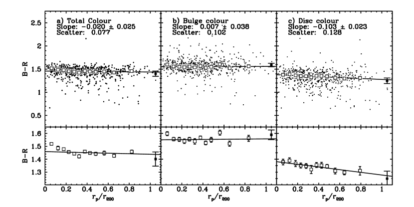
Figure 15: Total colour, bulge colour, and disc colour versus projected radius in units of $r_{200}$ for the $M_{R}<-19.5$ sample. The upper panels show individual points and medians (open squares). The filled square denotes the median for the field sample, and is placed arbitrarily at 1.05 $r/r_{200}$.

Before turning to the dependence of colours on measures of environment, we must first examine the possibility of luminosity segregation, because, if there were significant luminosity segregation in clusters, one might expect to see a colour-radius effect arising from the combination of luminosity segregation and the CMR. Fig. 14 shows magnitude as a function of radius. The brightest galaxies, with $M_{R}<-22$ appear to prefer $r_{\rm p}/r_{200}<0.6$. For the remainder of the galaxies, no evidence for luminosity segregation in our sample. This result is in agreement with the recent studies (Adami et al., 1998; Biviano et al., 2002; Pracy et al., 2005; Mercurio et al., 2006; von der Linden et al., 2010). Furthermore, when if we subtract the CMR from the observed colours and look for the dependence of the colour residuals on radius, we find trends of similar significance to those found below. Hence for simplicity, we simply fit colour as a function of cluster-centric radius.

Figure 15 shows total, bulge and disc colours versus projected cluster-centric radius in units of the virial radius: $\mbox{$r_{\rm p}$}/r_{200}$, Here, only the data with $M_{R}<-19.5$ are used. The left panel shows the total colour as a function of radius. The slope of the fit to median colours is $-0.020\pm 0.025$. The bulge colours are shown in the middle panel. The slope of the bulge-colour-radius relation is not statistically significant. Finally, the disc colours are shown in the right-hand panel, where the radial slope is statistically significant at the 4.5$\sigma$ level: $-0.103\pm 0.023$. These fits, as well as those described below, are summarized in Table 3.

Visual examination of Fig. 15 may hint that much of the change in disc colours is due to a tail of blue discs in the outskirts of clusters. However, recall that we are fitting the median colour (not the mean) and this is much less sensitive to outliers. The disc colours for “core” ($\mbox{$r_{\rm p}$}<0.3r_{200}$) and “outskirt” ($0.3<r_{p}/r_{200}<1$) samples are shown in Fig. 16. This confirms that, while such a blue tail does exist, the peak of the distribution is also shifted to the blue in the “outskirts” bin. Moreover, this trend continues to the field: the peak of the colour distribution shifts blueward, and the fraction of very blue discs ($\mbox{$B-R$}<1$) increases. A Kolmogorov-Smirnov (K-S) test shows that the “core” bin is significantly different from both the “outskirts” bin and from the field, at 99.92% and 99.5% confidence levels respectively. Thus there is a clear difference between the cores of rich clusters and the field.

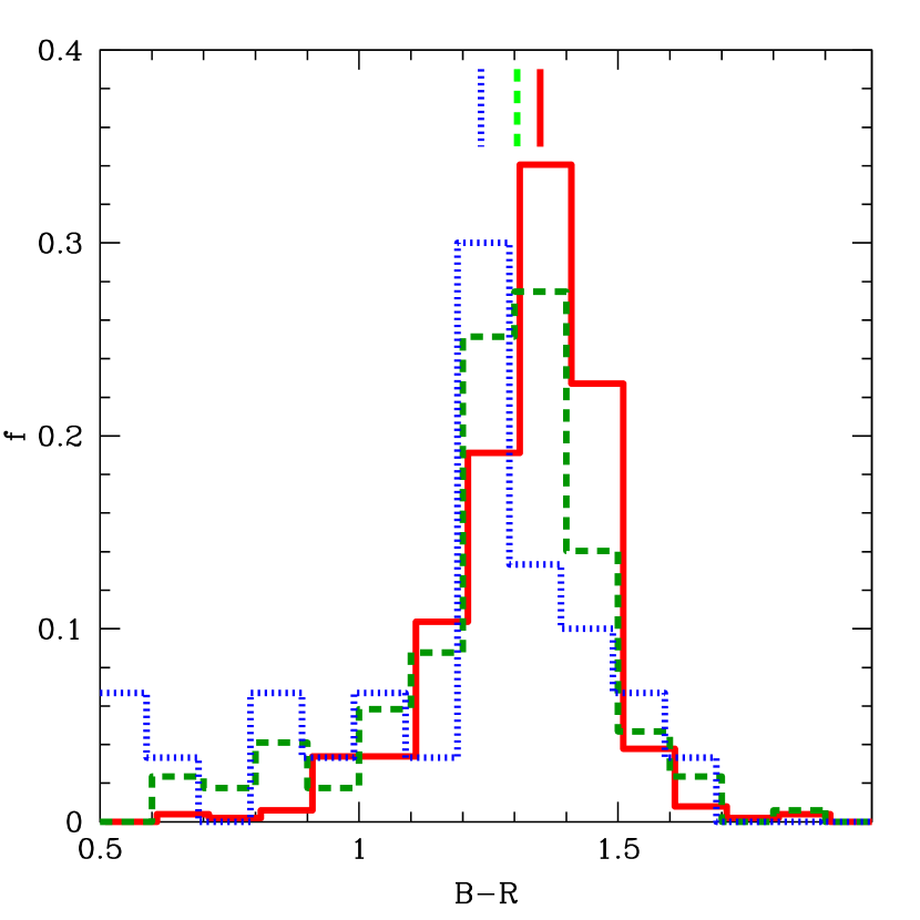
Figure 16: Histograms of disc colour for two radial ranges $\mbox{$r_{\rm p}$}<0.3r_{200}$ (red solid) for $\mbox{$r_{\rm p}$}>0.3r_{200}$ (green dashed) and in the field (blue dotted). The vertical marks indicate the median colours of each sample.

We have also performed the same bulge and disc fits as a function of $\log(\mbox{$r_{\rm p}$}/r_{200})$ (see Table 3). This functional form gives greater leverage to the innermost regions. For this parametrization, the radial dependence of the total colour is highly significant: the slope is $-0.092\pm 0.013$ per decade in radius. Furthermore, with this parametrization, the bulge colour dependence is also statistically significant ($-0.046\pm 0.018$), while the disc dependence ($-0.065\pm 0.015$) remains significant. The difference between the results from the linear fit and the logarithmic fit arise from the “core” regions $\mbox{$r_{\rm p}$}\mathrel{\hbox{\hbox to0.0pt{\hbox{\lower 4.0pt\hbox{$\sim$}}\hss}\hbox{$<$}}}0.2\,r_{200}$, where bulge colours (and consequently the total colours) appear to be somewhat redder than at larger annuli.

Table 3: Galaxy colours and properties as a function of environment. Slopes that differ from zero at greater than $3\sigma$ significance level are shown in bold type.

$y$	$x$	slope
$M_{R}$	$r_{p}/r_{200}$	$0.063$$\pm$	$0.194$
$B/T$	$r_{p}/r_{200}$	$0.004$$\pm$	$0.061$
Total Colour	$r_{p}/r_{200}$	$-0.020$$\pm$	$0.025$
Bulge Colour	$r_{p}/r_{200}$	$0.007$$\pm$	$0.038$
Disc Colour	$r_{p}/r_{200}$	$\mathbf{-0.103}$$\pm$	$\mathbf{0.023}$
$M_{R}$	$\log(r_{p}/r_{200})$	$-0.182$$\pm$	$0.113$
$B/T$	$\log(r_{p}/r_{200})$	$\mathbf{-0.108}$$\pm$	$\mathbf{0.033}$
Total Colour	$\log(r_{p}/r_{200})$	$\mathbf{-0.092}$$\pm$	$\mathbf{0.013}$
Bulge Colour	$\log(r_{p}/r_{200})$	$-0.046$$\pm$	$0.018$
Disc Colour	$\log(r_{p}/r_{200})$	$\mathbf{-0.065}$$\pm$	$\mathbf{0.015}$
$M_{R}$	$\log(\Sigma_{5})$	$0.054$$\pm$	$0.064$
$B/T$	$\log(\Sigma_{5})$	$0.048$$\pm$	$0.019$
Total Colour	$\log(\Sigma_{5})$	$\mathbf{0.032}$$\pm$	$\mathbf{0.008}$
Bulge Colour	$\log(\Sigma_{5})$	$0.006$$\pm$	$0.014$
Disc Colour	$\log(\Sigma_{5})$	$\mathbf{0.050}$$\pm$	$\mathbf{0.013}$

We have also attempted to extend this analysis to fainter magnitudes but found that, when the sample is restricted to only the three clusters complete to $M_{R}<-18$, the error bars on the slopes are considerably (a factor 2-3 times) larger and so no firm conclusions can be drawn.

6.2 Density as an Environment Indicator

The cluster-centric radius is a reasonable proxy on average for the depth of the cluster potential well, but in reality clusters are built from groups and singles (see McGee et al., 2009, for a detailed discussion.). If the environmental influences are attributable to a given galaxy’s previous (“group-like”) environment (“pre-processing”) then an environmental indicator based on the local density might be more sensitive to such effects.

To test this we define the local density $\Sigma_{5}$ as follows. Using galaxies brighter than our absolute magnitude limit of $-19.5$, we find the distance to the fifth nearest neighbor in the cluster and compute the density using this radius. It turns out that this definition is almost identical (within a few hundredths of a magnitude) to the limit used by Balogh et al. (2004), who used SDSS $r$ mags. However, rather than defining the density within a $\pm 1000\>\mbox{\rm km~{}s\mbox{${}^{-1}$}}$ redshift slice, we simply consider only galaxies that are clusters members.

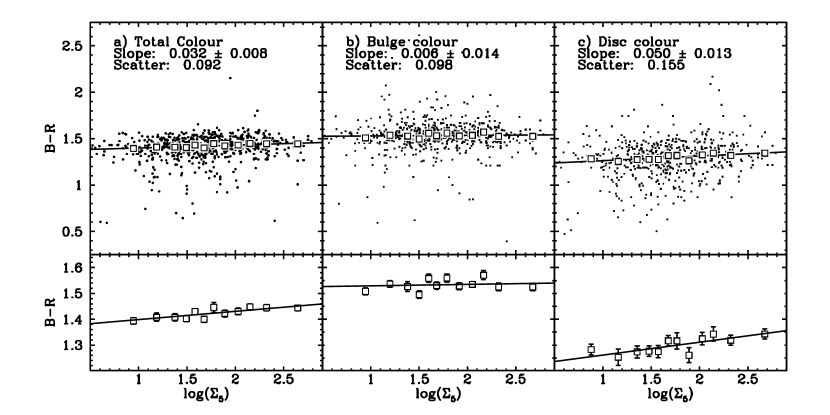
Figure 17: Total colour, bulge colour, and disc colour versus projected density.

As seen in Figure 17, the total colour varies as $0.032\pm 0.008$ per dex in density, in the expected sense that galaxies in higher density environments are redder. The bulge colour slope is not statistically significant ($0.006\pm 0.019$) but the disc colour slope is $0.050\pm 0.013$, significant at the 3.9 $\sigma$ level. The significance of the trends with density are similar to, or slightly lower in significance than the radial trends as a function of $\log(\mbox{$r_{\rm p}$}/r_{200})$, suggesting that these two measures of environment are largely degenerate when applied to rich clusters.

7 Discussion

7.1 Bulges

The bulge colours have show no dependence on environment from the cores of rich clusters to the field. At face value, this is compatible with the results from morphologically-selected samples. For example, van Dokkum et al. (1998) found no clustercentric variation in their E sample (although they did find a trend for their S0 sample). Hogg et al. (2004) found a very weak dependence of the peak of the colour distribution of Sérsic $n>2$ galaxies with density. Finally, in a cluster at $z=0.83$, Koo et al. (2005) also found that bulge colours were insensitive to cluster-centric radius.

However, we note that it is possible for the stellar populations of bulges to change in such a way as to preserve $B-R$ colour. For this to occur, changes in metallicity and age would have to be coordinated such that $(\Delta Z)/Z=-0.7(\Delta\mathrm{Age})/\mathrm{Age}$ (Worthey, 1994). In fact, an anti-correlation with exactly such a slope is indeed observed from spectroscopic analyses which break the age-metallicity degeneracy (Trager et al., 2000; Smith et al., 2008a). So it is possible that there is greater variation in the stellar populations of bulges than their colours suggest.

7.2 Disc fading

The dependence of disc colour on radius strongly suggests a scenario in which their star formation has been shut off by the cluster environment, after which the discs fade and redden. It is interesting to determine whether this process is abrupt, as one might expect if the cold gas is stripped by ram pressure, or slower, as might be expected in the “strangulation” scenario (Larson et al., 1980), in which the hot gas halo is stripped, but the cold gas remains to fuel star formation. The former scenario certainly exists: Smith et al. (2010) found that at least 1/3 of blue galaxies in the 1 $h\mbox{${}^{-1}$}$Mpc-radius core of Coma show UV tails extending from the disk suggestive of star formation during ram pressure stripping, and the direction of the tails suggests that the stripping is occurring on infall. It is not clear, however, how efficient and how rapid this process is. Evidence for a slower “strangulation” mechanism is favoured by a comparison of models with red and blue fractions (Font et al., 2008; van den Bosch et al., 2008; Weinmann et al., 2009; McGee et al., 2009).

We have found that the difference in median colour between discs at the centre of the cluster and those at the virial radius is $0.103\pm 0.023$ magnitudes in $B-R$. It is interesting to see if this colour difference can be reproduced with simple infall models in which star formation is truncated as the disc falls into the cluster. We use the simulations of Gao et al. (2004) to associate a given cluster-centric radius with a median infall time. Their Figure 15 suggests that while objects in the centre of the cluster were accreted at $z=1$ (a lookback time of 7.7 Gyr), those at the virial radius typically were accreted at $z\sim 0.4$ (4.3 Gyr ago).

If we assume that solar metallicity discs began forming stars at 10 Gyr ago at a continuous rate until crossing the cluster virial radius, followed by abrupt quenching, we obtain a colour of $1.43$ for the disc in the centre of the cluster, in reasonable agreement with the median observed value of $1.38$. However, at the virial radius, the predicted colour is $1.40$, which is quite red compared to the observed colour of $1.28$. Put another way, the predicted colour difference (a more robust quantity than the absolute colour) is $0.03$ whereas the observed value is $0.10\pm 0.02$. If we instead adopt a “strangulation” scenario for the disc in which star formation is not cut off abruptly, but instead declines with an exponential decay rate of 1 Gyr after infall, the predicted colour difference between a disc at the centre and one at the virial radius is $0.07$. This is in better agreement with the observed radial gradient in disc colour.

However, the above naive interpretation is significantly complicated by projection effects. There are two factors at play: first, an intrinsic three-dimensional colour gradient will be flattened when viewed in projection; second, there will be contamination by infalling field galaxies that are outside the virial radius but which appear within the virial radius in projection (and which have sufficiently low velocities to pass the $\pm 3\sigma_{\rm cl}$ clipping). These field interlopers are found in the outer regions and so will steepen the observed colour gradient. The fraction of such interlopers is difficult to determine. Mamon et al. (2010) estimate that the fraction of such interlopers is a strong function of projected radius. More specifically, for the subsample with $r_{p}>0.3r_{200}$, one might expect $\sim 33\%$ of objects to lie beyond the virial radius in three dimensions (G. Mamon, private communication). As a further complication, most of these “interlopers” will be infalling blue galaxies, but some may be “backsplash” galaxies which have passed through the centre of the cluster and have exited the virial radius.

We can test the null hypothesis that there is no intrinsic variation within the cluster virial radius. Specifically, we simulate the colour distribution of the outer radial bin with a mixture of the disc colours from the “core” bin (67%) with 33% contamination from the field discs. While the median colour of this simulated population is slightly redder than the observations, a K-S test shows that there is no significant difference between it and the observed distribution of disc colours in the outer radial bin. Thus we cannot rule out the hypothesis that the reddening begins beyond the virial radius. Nevertheless, the data do not exclude some reddening within the cluster itself: indeed a better fit is obtained if we assume that, intrinsically, the core galaxies are redder than the outskirt galaxies by 0.03 mag (in rough agreement with the “abrupt quenching” model discussed above). In summary, given the uncertainties associated with the interloper contamination fractions, and with the small size of the comparison field sample, it is difficult to decontaminate the cluster samples with sufficient accuracy in order to determine which scenario (abrupt quenching or strangulation) is at play. Nevertheless, we emphasize that there is indeed a difference between the disc colours of cluster-core galaxies and those at larger radii.

7.3 Implications for the Morphology-Density Relation

In the previous section, we showed that the data are consistent with a scenario in which the disc component fades within the cluster environment. Is this disc fading consistent with the buildup of the morphology-density relation? More specifically, are S0s formed by spirals after their discs fade and their spiral density waves are damped?

To address this question, we first need to estimate the amount of fading. Comparing a hypothetical field spiral where the disc continues forming stars at a constant rate to one which was truncated 6 Gyr ago, the models of Maraston (2005) predict a difference of a factor of $\sim 2.5$ in the $R$-band stellar mass-to-light ratio and a factor $\sim 4$ in the $B$-band. Thus, assuming the bulge is unaffected by environment, as a galaxy’s disc fades, the total $R$ luminosity will drop by a factor less than 2.5, and $B/T$ will increase by a factor up to 2.5. General support for this picture comes from studies (Neistein et al., 1999; Bedregal et al., 2006) which have shown that the S0 Tully & Fisher (1977, hereafter TF) relation is approximately consistent with being a faded version of the spiral TF relation.

However, there are problems with applying this simple fading scenario to map the field population into the cluster population as a whole. One problem arises when comparing the cluster $B/T$ distribution to that in the field. In Fig. 8, we showed the field $B$-band $B/T$ distribution from Allen et al. (2006), which has a large excess of late types with $\mbox{$B/T$}<0.1$ (and many with no bulge at all). As noted above, in the $B$-band, the fading might be as much as a factor of 4 between the field and the cluster. Thus field late-type spirals which would have had $\mbox{$B/T$}<0.1$ had their star formation continued, might appear as $\mbox{$B/T$}\sim 0.2$ if their star formation was truncated at cluster infall. However, Fig. 8 does not show an excess of objects with $\mbox{$B/T$}\sim 0.2$, but rather a broad distribution peaking at $\mbox{$B/T$}\sim 0.5$ in the $B$-band. Thus in order to create the cluster $B/T$ histogram from that in the field, one needs to either transform the discs of late-type spirals into bulges, perhaps by “harassment” (Moore et al., 1998), or to remove the very low $B/T$ objects from the distribution entirely, either by fading them below the magnitude limit or by destroying these galaxies.

A further problem with the scenario in which all S0s are formed from present-day spirals is the observation that the bulges of S0s are larger and brighter than those of spirals (Dressler, 1980; Burstein et al., 2005; Christlein & Zabludoff, 2004). Therefore it seems that while the brighter S0s in present day clusters are unlikely to be the faded remnants of today’s disc galaxies, this does not exclude fading as possible mechanism for creating lower-luminosity S0s. Whether the brighter cluster S0s are consistent with being the faded versions of higher-redshift spirals remains to be seen.

8 Conclusions

We have shown that the “tilt” of the total-light CMR is driven primarily by the tilt of CMR of the bulges (but not by the discs), and to a lesser extent, by a change in the $B/T$ ratio as a function of magnitude along the red-sequence. The tilt of the CMR is therefore due primarily to stellar population changes in the bulge as a function of magnitude or $\sigma$.

In clusters, we find that discs in $L_{*}$ galaxies are $\sim 0.25$ magnitudes bluer than bulges. If we assume that discs have solar metallicity, their colours are consistent with an SSP age of 4.5 Gyr.

Although bulge colours are insensitive to environment, the disc colours show a statistically significant dependence on cluster-centric radius in the sense that discs are bluer at the virial radius by $\sim 0.103\pm 0.023$ magnitudes in $B-R$ compared to their counterparts of the same total magnitude in the cluster centre. This effect drives the total-colour–radius relation noted by previous authors. A straightforward interpretation of this result is that it is due to the quenching of star formation in the disc upon cluster infall.

In summary, the physical processes that affect star formation in bulges are mass-dependent, and presumably primarily internal, whereas star formation in the disc shows little dependence on mass, but a strong dependence on environment as parametrized by cluster-centric radius.

Appendix A Ages and Metallicities of Bulges and Discs from Colours and Spectra

Bulges and discs have different colours, presumably due to differing stellar populations. Due to degeneracies, it is difficult to measure both ages and metallicities from optical colours alone. Spectra allow one to break this degeneracy, and ideally, one would use IFU spectra to obtain spatially resolved ages and metallicties, but, at present, such IFU samples remain small and somewhat heterogeneous (e.g. Rawle et al., 2008; Kuntschner et al., 2010). However, the NFPS contains spectra and stellar absorption linestrengths for 4097 red galaxies obtained from 2 arcsecond diameter fibres. From the linestrengths, a strong “downsizing” trend – younger ages in less massive galaxies – was found (Nelan et al., 2005). However, if the disc is younger than the bulge, and if $B/T$ varies along the red-sequence, some of this trend may be due to variations in the fraction of central spectra arising from discs.

It is possible to use these spectra to infer bulge ages if we make some assumptions about the disc properties. Since the disc colour is independent of magnitude and $\sigma$, we will assume that discs have an SSP age of 4.5 Gyr, solar metallicty and solar ratios of $\alpha$-elements to iron. These parameters are chosen because they yield Maraston (1998) model colours (assuming a (Kroupa, 2001) initial mass function), for the disc consistent with their median observed colour of 1.353. We will then model the contributions to the spectra from the bulge and disc components, and fit the stellar population parameters of the bulge using the central spectra. We will do this for subsamples binned by velocity dispersion, rather than magnitude because it has been shown that velocity dispersion, $\sigma$, is the driving parameter of the stellar populations (Smith et al., 2009a; Graves et al., 2009).

The central 2 arcsecond aperture contains a mixture of bulge and disc light, and so careful modelling is needed. In order to assess the contribution from bulge and disc to the central spectra, we use the GIM2D parameters to first calculate the bulge and disc light within a 2 arcsecond diameter aperture (matching the NFPS spectra), assuming that the exponential disc light can be extrapolated to the center. We have found that, not only is $\sigma$ strongly correlated with stellar populations, it is also strongly correlated with morphology: Fig. 18 shows $B/T$ and the aperture $B/T$_ap, as a function of $\sigma$. Note the strong correlation and relatively low scatter (compare with the weak trend and high scatter in $B/T$ versus magnitude in Fig. 6). Nevertheless, at all $\log(\sigma)>1.8$, the central light is always dominated by the bulge. Thus for each $\sigma$ bin, we know $B/T$_ap from Fig. 18.

We proceed to model the ages and metallicities as follows. Given the disc age and metallicities, we vary the bulge age, metallicity and $\alpha$-enhancement. For each choice of bulge parameters, we calculate the stellar mass-to-light ratios of the bulge and disc components and, given the fraction of light in the bulge from $\mbox{$B/T$}_{ap}$, we solve for the stellar mass fraction in the bulge and in the disc components. We use the composite stellar population models of Allanson et al. (2009), which in turn are based on Thomas et al. (2003, 2004), to calculate spectral linestrength indices for the two-component model and compare these to the mean NFPS linestrengths for the same $\sigma$ bin, and then minimize to find the best-fit bulge age and metallicity.

The resulting bulge ages and metallicities as a function of $\sigma$ are shown in Fig. 19. We show results for two data samples: the NFPS (Nelan et al., 2005); and 3 clusters in the Shapley concentration (Smith et al., 2007), which are also observed through a 2 arcsecond fibre, and are at a similar distance to the NFPS clusters studied in this paper. In both cases, the effect of including a 4.5 Gyr disc component is to shift the bulges to older ages, typically by $1-2$ Gyr, compared to simple single-component SSP fits. There is some disagreement between the two samples for the lowest $\log\sigma\sim 1.8$ bin, for which the NFPS requires bulge ages $\sim 4.5$ Gyr, whereas the Shapley sample prefers ages $\sim 6.5$ Gyr. For both samples, the “downsizing trend”, in which bulges with larger velocity dispersions are older, is present in bulge components.

Of course, this result is based on the assumption that disc surface brightness profile continues to be an exponential right to the centre of the galaxy. If the surface brightness profile flattens towards the centre, as is common in S0’s (Freeman, 1970), then the disc contribution is reduced compared to the bulge, and our conclusion regarding bulge downsizing is strengthened. It is, of course, in principle also possible that disc age does vary along the sequence, and that metallicity and/or dust conspire to achieve a disc colour which is independent of magnitude or $\sigma$, but such scenarios would require fine-tuning and so seem rather contrived. Thus we conclude that the variation in bulge metallicity along the red-sequence appears to be relatively less important than bulge age in driving the bulge CSR (and hence CMR).

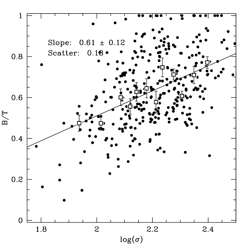
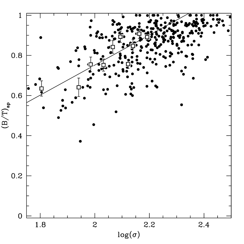
Figure 18: $R-$band $B/T$ as a function of velocity dispersion, $\sigma$. The left panel shows $B/T$, whereas the right panel shows the $B/T$_ap, the $B/T$obtained from the light within a 2 arcsecond diameter aperture, chosen to match fibre spectroscopy. As in other plots, the solid squares show medians fo bins of $\sigma$. Note the tight correlation between $\log\sigma$ and $B/T$.

Figure 19: Bulge age as a function of bulge metallicity. The left panel shows fits to the NFPS central linestrength data, assuming a 4.5 Gyr solar metallicity disc (indicated by the solid circle). Contours indicate 1 and 2 $\sigma$ confidence levels on two parameters jointly for bins with $\langle\log\sigma\rangle=1.94,2.09,2.17,2.26,2.39$ from bottom left to top right. The base of each arrow shows the SSP parameters if we assume only a single component SSP as in Nelan et al. (2005), whereas the tip of the arrow shows the best fit bulge parameters of the bulge+disc model. The right panel is the same except for the data from 3 clusters in the Shapley Concentration from Smith et al. (2007), in comparison to single-component SSPs from Allanson et al. (2009) for bins $\langle\log\sigma\rangle=1.71,1.84,2.02,2.16,2.31$, from leftmost to upper right. Note that the central spectra require that the bulge component of lower $\sigma$ galaxies is younger than that found in larger $\sigma$ galaxies (bulge “downsizing”).

References

- Abazajian et al. (2004) Abazajian K., et al., 2004, AJ, 128, 502
- Abraham et al. (1996) Abraham R. G., Smecker-Hane T. A., Hutchings J. B., Carlberg R. G., Yee H. K. C., Ellingson E., Morris S., Oke J. B., Rigler M., 1996, ApJ, 471, 694
- Adami et al. (1998) Adami C., Biviano A., Mazure A., 1998, A&A, 331, 439
- Allanson et al. (2009) Allanson S. P., Hudson M. J., Smith R. J., Lucey J. R., 2009, ApJ, 702, 1275
- Allen et al. (2006) Allen P. D., Driver S. P., Graham A. W., Cameron E., Liske J., de Propris R., 2006, MNRAS, 371, 2
- Andreon et al. (2006) Andreon S., Quintana H., Tajer M., Galaz G., Surdej J., 2006, MNRAS, 365, 915
- Balcells & Peletier (1994) Balcells M., Peletier R. F., 1994, AJ, 107, 135
- Balogh et al. (2004) Balogh M. L., Baldry I. K., Nichol R., Miller C., Bower R., Glazebrook K., 2004, ApJL, 615, L101
- Balogh & Morris (2000) Balogh M. L., Morris S. L., 2000, MNRAS, 318, 703
- Balogh et al. (2000) Balogh M. L., Navarro J. F., Morris S. L., 2000, ApJ, 540, 113
- Bamford et al. (2009) Bamford S. P., Nichol R. C., Baldry I. K., Land K., Lintott C. J., Schawinski K., Slosar A., Szalay A. S., Thomas D., Torki M., Andreescu D., Edmondson E. M., Miller C. J., Murray P., Raddick M. J., Vandenberg J., 2009, MNRAS, 393, 1324
- Barazza et al. (2009) Barazza F. D., Wolf C., Gray M. E., Jogee S., Balogh M., McIntosh D. H., Bacon D., Barden M., Bell E. F., Böhm A., Caldwell J. A. R., Häussler B., Heiderman A., Heymans C., Jahnke K., van Kampen E., Lane K., Marinova I., Meisenheimer K., Peng C. Y., Sanchez S. F., Taylor A., Wisotzki L., Zheng X., 2009, A&A, 508, 665
- Bedregal et al. (2006) Bedregal A. G., Aragón-Salamanca A., Merrifield M. R., 2006, MNRAS, 373, 1125
- Bernardi et al. (2006) Bernardi M., Nichol R. C., Sheth R. K., Miller C. J., Brinkmann J., 2006, AJ, 131, 1288
- Bertin & Arnouts (1996) Bertin E., Arnouts S., 1996, A&AS, 117, 393
- Biviano et al. (2002) Biviano A., Katgert P., Thomas T., Adami C., 2002, A&A, 387, 8
- Boselli & Gavazzi (2006) Boselli A., Gavazzi G., 2006, PASP, 118, 517
- Bower et al. (1992) Bower R. G., Lucey J. R., Ellis R. S., 1992, MNRAS, 254, 601
- Burstein et al. (2005) Burstein D., Ho L. C., Huchra J. P., Macri L. M., 2005, ApJ, 621, 246
- Butcher & Oemler (1984) Butcher H., Oemler A., 1984, ApJ, 285, 426
- Caon et al. (1990) Caon N., Capaccioli M., Rampazzo R., 1990, A&AS, 86, 429
- Carlberg et al. (1997) Carlberg R. G., Yee H. K. C., Ellingson E., 1997, ApJ, 478, 462
- Carter et al. (2002) Carter D., Mobasher B., Bridges T. J., Poggianti B. M., Komiyama Y., Kashikawa N., Doi M., Iye M., Okamura S., Sekiguchi M., Shimasaku K., Yagi M., Yasuda N., 2002, ApJ, 567, 772
- Cayatte et al. (1990) Cayatte V., van Gorkom J. H., Balkowski C., Kotanyi C., 1990, AJ, 100, 604
- Christlein & Zabludoff (2003) Christlein D., Zabludoff A. I., 2003, ApJ, 591, 764
- Christlein & Zabludoff (2004) —, 2004, ApJ, 616, 192
- Davies & Lewis (1973) Davies R. D., Lewis B. M., 1973, MNRAS, 165, 231
- de Jong et al. (2004) de Jong R. S., Simard L., Davies R. L., Saglia R. P., Burstein D., Colless M., McMahan R., Wegner G., 2004, MNRAS, 355, 1155
- de Vaucouleurs et al. (1991) de Vaucouleurs G., de Vaucouleurs A., Corwin H. G., Buta R. J., Paturel G., Fouqué P., 1991, Third Reference Catalogue of Bright Galaxies. Springer-Verlag
- Djorgovski & Davis (1987) Djorgovski S., Davis M., 1987, ApJ, 313, 59
- D’Onofrio (2001) D’Onofrio M., 2001, MNRAS, 326, 1517
- Dressler (1980) Dressler A., 1980, ApJ, 236, 351
- Dressler et al. (1987) Dressler A., Lynden-Bell D., Burstein D., Davies R. L., Faber S. M., Terlevich R., Wegner G., 1987, ApJ, 313, 42
- Dressler et al. (1997) Dressler A., Oemler A. J., Couch W. J., Smail I., Ellis R. S., Barger A., Butcher H., Poggianti B. M., Sharples R. M., 1997, ApJ, 490, 577
- Driver et al. (2007) Driver S. P., Popescu C. C., Tuffs R. J., Liske J., Graham A. W., Allen P. D., de Propris R., 2007, MNRAS, 563
- Fasano et al. (2000) Fasano G., Poggianti B. M., Couch W. J., Bettoni D., Kjærgaard P., Moles M., 2000, ApJ, 542, 673
- Font et al. (2008) Font A. S., Bower R. G., McCarthy I. G., Benson A. J., Frenk C. S., Helly J. C., Lacey C. G., Baugh C. M., Cole S., 2008, MNRAS, 389, 1619
- Freeman (1970) Freeman K. C., 1970, ApJ, 160, 811
- Frei & Gunn (1994) Frei Z., Gunn J. E., 1994, AJ, 108, 1476
- Gallagher & Ostriker (1972) Gallagher III J. S., Ostriker J. P., 1972, AJ, 77, 288
- Gao et al. (2004) Gao L., White S. D. M., Jenkins A., Stoehr F., Springel V., 2004, MNRAS, 355, 819
- Giovanelli & Haynes (1985) Giovanelli R., Haynes M. P., 1985, ApJ, 292, 404
- Graves et al. (2009) Graves G. J., Faber S. M., Schiavon R. P., 2009, ApJ, 693, 486
- Gunn & Gott (1972) Gunn J. E., Gott J. R. I., 1972, ApJ, 176, 1
- Gutiérrez et al. (2004) Gutiérrez C. M., Trujillo I., Aguerri J. A. L., Graham A. W., Caon N., 2004, ApJ, 602, 664
- Haynes et al. (1984) Haynes M. P., Giovanelli R., Chincarini G. L., 1984, ARA&A, 22, 445
- Hogg et al. (2004) Hogg D. W., Blanton M. R., Brinchmann J., Eisenstein D. J., Schlegel D. J., Gunn J. E., McKay T. A., Rix H.-W., Bahcall N. A., Brinkmann J., Meiksin A., 2004, ApJL, 601, L29
- Holmberg (1958) Holmberg E., 1958, Meddelanden fran Lunds Astronomiska Observatorium Serie II, 136, 1
- Hubble & Humason (1931) Hubble E., Humason M. L., 1931, ApJ, 74, 43
- Jorgensen & Franx (1994) Jorgensen I., Franx M., 1994, ApJ, 433, 553
- Katgert et al. (1998) Katgert P., Mazure A., den Hartog R., Adami C., Biviano A., Perea J., 1998, A&AS, 129, 399
- Kennicutt (1983) Kennicutt Jr. R. C., 1983, AJ, 88, 483
- Kent (1985) Kent S. M., 1985, ApJS, 59, 115
- Koo et al. (2005) Koo D. C., Datta S., Willmer C. N. A., Simard L., Tran K.-V., Im M., 2005, ApJL, 634, L5
- Kroupa (2001) Kroupa P., 2001, MNRAS, 322, 231
- Kuntschner et al. (2010) Kuntschner H., Emsellem E., Bacon R., Cappellari M., Davies R. L., de Zeeuw P. T., Falcón-Barroso J., Krajnović D., McDermid R. M., Peletier R. F., Sarzi M., Shapiro K. L., van den Bosch R. C. E., van de Ven G., 2010, ArXiv e-prints
- Landolt (1992) Landolt A. U., 1992, AJ, 104, 340
- Larson et al. (1980) Larson R. B., Tinsley B. M., Caldwell C. N., 1980, ApJ, 237, 692
- López-Cruz et al. (2004) López-Cruz O., Barkhouse W. A., Yee H. K. C., 2004, ApJ, 614, 679
- MacArthur et al. (2004) MacArthur L. A., Courteau S., Bell E., Holtzman J. A., 2004, ApJS, 152, 175
- Mamon (1987) Mamon G. A., 1987, ApJ, 321, 622
- Mamon et al. (2010) Mamon G. A., Biviano A., Murante G., 2010, A&A, submitted
- Maraston (1998) Maraston C., 1998, MNRAS, 300, 872
- Maraston (2005) —, 2005, MNRAS, 362, 799
- Matković & Guzmán (2005) Matković A., Guzmán R., 2005, MNRAS, 362, 289
- McGee et al. (2009) McGee S. L., Balogh M. L., Bower R. G., Font A. S., McCarthy I. G., 2009, MNRAS, 400, 937
- McGee et al. (2008) McGee S. L., Balogh M. L., Henderson R. D. E., Wilman D. J., Bower R. G., Mulchaey J. S., Oemler Jr. A., 2008, MNRAS, 387, 1605
- McIntosh et al. (2004) McIntosh D. H., Rix H., Caldwell N., 2004, ApJ, 610, 161
- Mercurio et al. (2006) Mercurio A., Merluzzi P., Haines C. P., Gargiulo A., Krusanova N., Busarello G., Barbera F. L., Capaccioli M., Covone G., 2006, MNRAS, 368, 109
- Merritt (1984) Merritt D., 1984, ApJ, 276, 26
- Moore et al. (1998) Moore B., Lake G., Katz N., 1998, ApJ, 495, 139
- Neistein et al. (1999) Neistein E., Maoz D., Rix H., Tonry J. L., 1999, AJ, 117, 2666
- Nelan et al. (2005) Nelan J. E., Smith R. J., Hudson M. J., Wegner G. A., Lucey J. R., Moore S. A. W., Quinney S. J., Suntzeff N. B., 2005, ApJ, 632, 137
- Noordermeer & van der Hulst (2007) Noordermeer E., van der Hulst J. M., 2007, MNRAS, 376, 1480
- Peletier & Balcells (1996) Peletier R. F., Balcells M., 1996, AJ, 111, 2238
- Postman & Geller (1984) Postman M., Geller M. J., 1984, ApJ, 281, 95
- Pracy et al. (2005) Pracy M. B., Driver S. P., De Propris R., Couch W. J., Nulsen P. E. J., 2005, MNRAS, 364, 1147
- Proctor et al. (2004) Proctor R. N., Forbes D. A., Hau G. K. T., Beasley M. A., De Silva G. M., Contreras R., Terlevich A. I., 2004, MNRAS, 349, 1381
- Rawle et al. (2008) Rawle T. D., Smith R. J., Lucey J. R., Swinbank A. M., 2008, MNRAS, 389, 1891
- Rines et al. (2003) Rines K., Geller M. J., Kurtz M. J., Diaferio A., 2003, AJ, 126, 2152
- Sandage & Visvanathan (1978) Sandage A., Visvanathan N., 1978, ApJ, 223, 707
- Schlegel et al. (1998) Schlegel D. J., Finkbeiner D. P., Davis M., 1998, ApJ, 500, 525
- Simard et al. (2002) Simard L., Willmer C. N. A., Vogt N. P., Sarajedini V. L., Phillips A. C., Weiner B. J., Koo D. C., Im M., Illingworth G. D., Faber S. M., 2002, ApJS, 142, 1
- Simien & de Vaucouleurs (1986) Simien F., de Vaucouleurs G., 1986, ApJ, 302, 564
- Smith et al. (2006) Smith R. J., Hudson M. J., Lucey J. R., Nelan J. E., Wegner G. A., 2006, MNRAS, 369, 1419
- Smith et al. (2004) Smith R. J., Hudson M. J., Nelan J. E., Moore S. A. W., Quinney S. J., Wegner G. A., Lucey J. R., Davies R. L., Malecki J. J., Schade D., Suntzeff N. B., 2004, AJ, 128, 1558
- Smith et al. (2010) Smith R. J., Lucey J. R., Hammer D., 2010, MNRAS, submitted
- Smith et al. (2007) Smith R. J., Lucey J. R., Hudson M. J., 2007, MNRAS, 381, 1035
- Smith et al. (2008a) —, 2008a, in IAU Symposium, Vol. 245, Formation and Evolution of Galaxy Bulges, pp. 411–414
- Smith et al. (2009a) —, 2009a, MNRAS, 400, 1690
- Smith et al. (2009b) Smith R. J., Lucey J. R., Hudson M. J., Allanson S. P., Bridges T. J., Hornschemeier A. E., Marzke R. O., Miller N. A., 2009b, MNRAS, 392, 1265
- Smith et al. (2008b) Smith R. J., Marzke R. O., Hornschemeier A. E., Bridges T. J., Hudson M. J., Miller N. A., Lucey J. R., Vázquez G. A., Carter D., 2008b, MNRAS, 386, L96
- Sullivan et al. (1981) Sullivan III W. T., Bates B., Bothun G. D., Schommer R. A., 1981, AJ, 86, 919
- Terndrup et al. (1994) Terndrup D. M., Davies R. L., Frogel J. A., Depoy D. L., Wells L. A., 1994, ApJ, 432, 518
- Thomas et al. (2003) Thomas D., Maraston C., Bender R., 2003, MNRAS, 339, 897
- Thomas et al. (2005) Thomas D., Maraston C., Bender R., de Oliveira C. M., 2005, ApJ, 621, 673
- Thomas et al. (2004) Thomas D., Maraston C., Korn A., 2004, MNRAS, 351, L19
- Trager et al. (2000) Trager S. C., Faber S. M., Worthey G., González J. J., 2000, AJ, 120, 165
- Tully & Fisher (1977) Tully R. B., Fisher J. R., 1977, A&A, 54, 661
- van den Bergh (1976) van den Bergh S., 1976, ApJ, 206, 883
- van den Bosch et al. (2008) van den Bosch F. C., Aquino D., Yang X., Mo H. J., Pasquali A., McIntosh D. H., Weinmann S. M., Kang X., 2008, MNRAS, 387, 79
- van Dokkum et al. (1998) van Dokkum P. G., Franx M., Kelson D. D., Illingworth G. D., Fisher D., Fabricant D., 1998, ApJ, 500, 714
- von der Linden et al. (2010) von der Linden A., Wild V., Kauffmann G., White S. D. M., Weinmann S., 2010, MNRAS, 404, 1231
- Weinmann et al. (2009) Weinmann S. M., Kauffmann G., van den Bosch F. C., Pasquali A., McIntosh D. H., Mo H., Yang X., Guo Y., 2009, MNRAS, 394, 1213
- Worthey (1994) Worthey G., 1994, ApJS, 95, 107