Hole spin relaxation in intrinsic and $p$-type bulk GaAs

Abstract

We investigate hole spin relaxation in intrinsic and $p$-type bulk GaAs from a fully microscopic kinetic spin Bloch equation approach. In contrast to the previous study on hole spin dynamics, we explicitly include the intraband coherence and the nonpolar hole-optical-phonon interaction, both of which are demonstrated to be of great importance to the hole spin relaxation. The relative contributions of the D’yakonov-Perel’ and Elliott-Yafet mechanisms on hole spin relaxation are also analyzed. In our calculation, the screening constant, playing an important role in the hole spin relaxation, is treated with the random phase approximation. In intrinsic GaAs, our result shows good agreement with the experiment data at room temperature, where the hole spin relaxation is demonstrated to be dominated by the Elliott-Yafet mechanism. We also find that the hole spin relaxation strongly depends on the temperature and predict a valley in the density dependence of the hole spin relaxation time at low temperature due to the hole-electron scattering. In $p$-type GaAs, we predict a peak in the spin relaxation time against the hole density at low temperature, which originates from the distinct behaviors of the screening in the degenerate and nondegenerate regimes. The competition between the screening and the momentum exchange during scattering events can also lead to a valley in the density dependence of the hole spin relaxation time in the low density regime. At high temperature, the effect of the screening is suppressed due to the small screening constant. Moreover, we predict a nonmonotonic dependence of the hole spin relaxation time on temperature associated with the screening together with the hole-phonon scattering. Finally, we find that the D’yakonov-Perel’ mechanism can markedly contribute to the hole spin relaxation in the low density case at moderate temperature and in the high density case at low temperature, where the Elliott-Yafet mechanism is suppressed due to the relatively weak scattering.

I Introduction

In the past decade, semiconductor spintronics, with the aim of realizing favourable devices for future application based on the spin degree of freedom, has attracted much attention.meier ; wolf ; spintronics ; korn ; wu One of the most critical challenges for such devices lies in the control of the spin lifetime, which is limited by the unavoidable spin relaxation and/or dephasing process in semiconductors. In this sense, understanding of the carrier spin relaxations and/or dephasings is a critical issue.spintronics ; korn ; wu ; chen ; sherman In bulk materials, the spin relaxation and/or dephasing properties of the electrons and the underlying physics have been well understood after a long-time research.seymour ; zerro ; kikkawa ; song ; teng ; oertel ; wu6 ; romer ; krauss2 ; shen However, the study on hole spin dynamics, which occurs on the time scale of the momentum scattering time (usually $<1$ ps), is fairly rare, partly because of the limited resolution on the detection of such an ultrafast process. To our best knowledge, the hole spin lifetime in bulk semiconductors was only measured in intrinsic GaAs at room temperature, which evaluated the spin relaxation time of the heavy hole ($\sim 110$ fs).hilton

One picture to explain the picosecond hole spin relaxation (HSR) time is the D’yakonov-Perel’-like description associated with the momentum scattering and the spin precession between the light-hole (LH) and heavy-hole (HH).culcer However, this picture works only if the broadening of the energy spectrum due to scattering is larger than the interband splitting, corresponding to the vicinity of the zone center. Otherwise, holes are driven to large momentum states where the degeneracy between the LH and HH bands is significantly lifted, hence it is more appropriate to treat the LH and HH bands separately. The HSR of the individual LH and HH bands was studied by Yu et al.,yu who obtained the accurate band structure from the tight-binding Hamiltonian with the spin-orbit coupling (SOC) and calculated the spin relaxation time of the LH (HH) as the inversion of the decay rate of the quasi-spin polarization, that is, the population difference of the LH (HH) between the two quasi-spin bands. The Elliott-Yafet (EY) mechanism,EY there described as the direct quasi-spin-flip scattering, was claimed to be the solo mechanism for the HH and the dominant one for the LH, while the D’yakonov-Perel’ (DP) mechanismDP treated as the intraband precession together with the quasi-spin-conserving scattering from the motional narrowing relation was found to be unimportant. Since the calculation was based on the single particle theory, the Coulomb interaction which has been demonstrated to result in intriguing many-body effects during electron spin dynamicswu ; wu1 ; wu2 ; glazov was missed in that work. Moreover, the HSR time was extracted from the quasi-spin polarization instead of the exact spin signal. The feasibility of this approach needs to be verified. In other words, the results obtained there is not exactly the HSR time, but the quasi-spin relaxation time. Recently, the hole spin dynamics in intrinsic bulk GaAs with the Coulomb interaction was microscopically investigated from an eight-band Kane Hamiltonian by Krauß et al.,krauss where the HSR time, directly from the decay of the hole spin expectation, was shown to be quite close to the experimental result. It was also shown that the HSR time can be slightly different from the quasi-spin relaxation time. Thus, it seems that ultrafast HSR in bulk zinc-blende semiconductors has been successfully interpreted theoretically. However, one may notice that the intraband coherence, i.e., the non-diagonal components of the density matrices was missing in that work, which actually will lead to two consequences: the exaggeration of the EY mechanism and the exclusion of the DP mechanism. Moreover, the nonpolar interaction of holes with transverse- and longitudinal-optical-phonons due to the deformation potential coupling, which was shown to produce a significant contribution on the charge dynamics of holes,langot ; scholz ; brudevoll was not included. In this sense, the results in Ref. krauss, should be reexamined.

In the present work, we employ the fully microscopic kinetic spin Bloch equations (KSBEs)wu ; wu1 ; wu6 ; wu9 ; wu10 to investigate the HSR due to the EY and DP mechanisms in intrinsic and $p$-type bulk GaAs. The EY mechanism here corresponds to the decay of the spin polarization solely due to the scattering associated with the interband mixing, between not only the HH and LH bands but also the conduction and valence bands; whereas the DP mechanism stands for the additional contribution by including the intraband spin precessions. We first analytically derive the valence band structure from the four-band Luttinger Hamiltonianluttinger together with the Dresselhaus SOC (Ref. dressel, ) due to the bulk inversion asymmetry in zinc-blende semiconductors. We demonstrate that the Dresselhaus SOC induces an intraband splitting between the two HH bands as well as the two LH bands with cubic wave-vector dependence, which supplies an additional HSR channel due to the DP mechanism. We find that the intraband splitting of the HH bands vanishes under the spherical approximation of the Luttinger Hamiltonian, and then the DP mechanism becomes irrelevant to the HH spin relaxation.yu This implies the limitation of such an approximation in calculating the HSR time. Therefore, we later obtain the intraband splitting and wave functions by diagonalizing the full eight-band ${\bf k}\cdot{\bf p}$ Hamiltonian beyond the spherical approximation. Then we calculate the HSR time from the KSBEs with the intraband coherence and all the relevant scatterings, such as the hole-impurity, hole-hole, hole-electron, hole-acoustic-phonon, polar and nonpolar hole-optical-phonon scatterings, explicitly included. In the intrinsic case at room temperature, the HSR is dominated by the EY mechanism and the HSR time shows good agreement with the experiment. We find that the HSR time can be significantly manipulated by changing the temperature and excitation density. In the $p$-type materials, we predict intriguing nonmonotonic behaviors of the HSR time in both the density and temperature dependences. We show that the nonmonotonic features reflect the role of the screening. Moreover, we find that the EY mechanism is usually the major mechanism of the HSR, but the DP mechanism can still be comparable with the EY mechanism in some special cases, such as the high density regime at low temperature and the low density regime at moderate temperature.

This paper is organized as follows. In Sec. II, we set up our model and derive the effective Dresselhaus field from the Luttinger Hamiltonian. The KSBEs are also constructed in this section. In Sec. III, we investigate the HSR in both intrinsic and $p$-type GaAs. The comparison of the calculations with and without the intraband coherence is given in this section to illustrate the role of the intraband coherence. The relative contributions of the DP and EY mechanisms are also discussed. Finally, we summarize in Sec. IV.

II Model and KSBE

To qualitatively analyze the band structure and the intraband splitting of the HH and LH bands, we start from the perturbation method with the $4\times 4$ Hamiltonian (in the basis of the eigenstates of $J_{z}$ with eigenvalues $\tfrac{3}{2}$, $\tfrac{1}{2}$, $-\tfrac{1}{2}$, and $-\tfrac{3}{2}$, in sequence) near the center of the Brillouin-zone

$${\mathcal{H}}_{8v8v}=\left(\begin{array}[]{cccc}F&H&I&0\\ H^{\ast}&G&0&I\\ I^{\ast}&0&G&-H\\ 0&I^{\ast}&-H^{\ast}&F\end{array}\right)+H_{8v8v}^{b}.$$ (5)

The first term on the right-hand side of the equation is the Luttinger Hamiltonian,luttinger where $F=-\frac{\hbar^{2}}{2m_{0}}[(\gamma_{1}+\gamma_{2})(k_{x}^{2}+k_{y}^{2})+(\gamma_{1}-2\gamma_{2})k_{z}^{2}]$, $G=-\frac{\hbar^{2}}{2m_{0}}[(\gamma_{1}-\gamma_{2})(k_{x}^{2}+k_{y}^{2})+(\gamma_{1}+2\gamma_{2})k_{z}^{2}]$, $H=2\sqrt{3}\frac{\hbar^{2}}{2m_{0}}\gamma_{3}(k_{x}-ik_{y})k_{z}$, and $I=\frac{\hbar^{2}}{2m_{0}}[\sqrt{3}\gamma_{2}(k_{x}^{2}-k_{y}^{2})-i2\sqrt{3}\gamma_{3}k_{x}k_{y}]$. $\gamma_{i}$ are Kohn-Luttinger parameters. We denote this term as $H_{0}$ in the following. The second term is the Dresselhaus SOC of the valence band, $H_{8v8v}^{b}={\bf h}_{\bf k}\cdot{\bf J}$, with the effective magnetic fielddressel ; winkler

$${\bf h}_{\bf k}=b_{41}^{8v8v}[k_{x}(k_{y}^{2}-k_{z}^{2}),k_{y}(k_{z}^{2}-k_{x}^{2}),k_{z}(k_{x}^{2}-k_{y}^{2})].$$ (6)

$J_{i}$ represent the spin-3/2 angular-momentum matrices. It is obvious that the band structure is mainly determined by $H_{0}$ in the vicinity of the zone-center. The energy spectrum from $H_{0}$ readsdressel2 ; chao

$$E_{h/l,\bf k} = -\tfrac{\hbar^{2}}{2m_{0}}\big{\{}\gamma_{1}k^{2}\mp[4\gamma^{2}_{2}k^{4}+12(\gamma_{3}^{2}-\gamma_{2}^{2})$$ (7)

$$\mbox{}\times(k_{x}^{2}k_{y}^{2}+k_{y}^{2}k_{z}^{2}+k_{z}^{2}k_{x}^{2})]^{\tfrac{1}{2}}\big{\}},$$

and the wave functions can be expressed by

$$\psi^{h/l}_{1}=(a_{1}^{h/l},b_{1}^{h/l},c_{1}^{h/l},0)^{T},$$ (8)

$$\psi^{h/l}_{2}=(0,c_{2}^{h/l},b_{2}^{h/l},a_{2}^{h/l})^{T}.$$ (9)

By identifying $\psi_{1}^{h/l}$ and $\psi_{2}^{h/l}$ as pseudo-spin-up and -down states separately, one obtains the effective magnetic field of the Dresselhaus SOC (${\mbox{\boldmath$\Omega$\unboldmath}}^{e}_{h/l}$) between them. Specifically, one rewrites $H_{8v8v}$ in the representation of $\{\psi_{i}^{h/l}\}$, and derives individual HH and LH blocks from the Löwdin partitioning methodlowdin upto the cubic power of the wave vector,

$$H_{h/l}({\bf k})=E_{h/l,{\bf k}}I_{2\times 2}+{\mbox{\boldmath$\Omega$\unboldmath}}^{e}_{h/l}({\bf k})\cdot{\mbox{\boldmath$\sigma$\unboldmath}},$$ (10)

where $\sigma$ are the Pauli matrices. The expressions of the effective magnetic field together with the coefficients $a_{i}^{h/l}$, $b_{i}^{h/l}$ and $c_{i}^{h/l}$ are given in Appendix A. The presence of the intraband splitting $\Delta E_{h/l,\bf k}=E^{2}_{h/l,\bf k}-E^{1}_{h/l,\bf k}=2|{\mbox{\boldmath$\Omega$\unboldmath}}^{e}_{h/l}({\bf k})|$ obviously indicates that the DP mechanism can contribute to the HSR in the presence of the scatterings.wu ; DP Interestingly, one finds ${\mbox{\boldmath$\Omega$\unboldmath}}^{e}_{h}$ vanishes once the spherical approximation (corresponding to $\gamma_{2}=\gamma_{3}$)balde ; schliemann is applied, which means that the contribution of the DP mechanism to the HH spin relaxation is lost within the spherical approximation scheme. In other words, the difference between $\gamma_{2}$ and $\gamma_{3}$, arising from the remote bands,winkler is important in counting the HH spin relaxation.

We should point out that the above perturbation approach gives the precise value of the intraband splitting only in the vicinity of the zone-center. For the regime far away from the center, the modification from the split-off and conduction bands should be considered. Therefore, the intraband splittings $\Delta E_{h/l,\bf k}$ are obtained from the diagonalization of the $8\times 8$ Kane Hamiltonian $H_{K}$ (Ref. kane, ) in our numerical calculation, that is, by solving the Schrödinger equation

$$H_{K}({\bf k})|\xi_{h/l,\bf k}^{i}\rangle=E^{i}_{h/l,{\bf k}}|\xi_{h/l,\bf k}^{i}\rangle,$$ (11)

with $i=1,2$. We define the single particle density matrices $\rho_{\bf k}^{h}$ as $4\times 4$ matrices in the helix representation,wu4 i.e., under the basis of the eigenstates $\{|\xi_{h,\bf k}^{1}\rangle,|\xi_{h,\bf k}^{2}\rangle,|\xi_{l,\bf k}^{1}\rangle,|\xi_{l,\bf k}^{2}\rangle\}$. The unitary transformation from the helix representation to the collinear representation, the basis of which is defined as the eigenstates of the angular momentum operator $J_{z}$, is given by

$$\rho_{\bf k}^{c}=U_{\bf k}\rho_{\bf k}^{h}U_{\bf k}^{\dagger},$$ (12)

with $U_{\bf k}=(\xi_{h,\bf k}^{1},\xi_{h,\bf k}^{2},\xi_{l,\bf k}^{1},\xi_{l,\bf k}^{2})$. The KSBEs in the helix representation from the nonequilibrium Green-function method readswu ; wu1

$$\partial_{t}\rho^{h}_{\bf k}=\partial_{t}\rho^{h}_{\bf k}\big{|}_{\rm coh}+\partial_{t}\rho^{h}_{\bf k}\big{|}_{\rm scat}.$$ (13)

The coherent term can be written as

$$\partial_{t}\rho^{h}_{{\bf k}}\big{|}_{\rm coh} = -i\big{[}\sum_{{\bf q}}V_{\bf q}S_{\bf k,k-q}\rho^{h}_{\bf k-q}S_{\bf k-q,k},\rho^{h}_{\bf k}\big{]}$$ (14)

$$\mbox{}-i\big{[}H^{h}({\bf k}),\rho^{h}_{\bf k}\big{]},$$

with $[,]$ representing the commutator. $S_{\bf k^{\prime},k}=U_{\bf k^{\prime}}^{\dagger}U_{\bf k}$. The first term on the right-hand side of the equation comes from the Coulomb Hartree-Fock contribution, which can be neglected for small spin polarization.wu In the helix frame, $H^{h}({\bf k})={\rm diag}(E_{h,\bf k}^{1},E_{h,\bf k}^{2},E_{l,\bf k}^{1},E_{l,\bf k}^{2})$, and Eq. (14) then can be rewritten as $\partial_{t}\rho_{\bf k}^{h}(m,n)\big{|}_{\rm coh}=-i\rho_{\bf k}^{h}(m,n)(E_{m,{\bf k}}-E_{n,{\bf k}})$. The scattering term is given bywu4

$$\partial_{t}\rho_{\bf k}^{h}\big{|}_{\rm scat}=-\pi n_{i}\sum_{{\bf q}\eta\eta^{\prime}}|U^{i}_{\bf q}|^{2}\delta(E_{\eta^{\prime}{\bf k-q}}-E_{\eta{\bf k}})S_{\bf k,k-q}$$

$$\mbox{}\times\big{[}\rho_{\bf k-q}^{h,>}T_{\bf k-q}^{\eta^{\prime}}S_{\bf k-q,k}T_{\bf k}^{\eta}\rho_{\bf k}^{h,<}-\rho_{\bf k-q}^{h,<}T_{\bf k-q}^{\eta^{\prime}}S_{\bf k-q,k}T_{\bf k}^{\eta}\rho_{\bf k}^{h,>}\big{]}$$

$$\mbox{}-\pi\sum_{{\bf q}\eta\eta^{\prime}\lambda}|M_{{\bf q},\lambda}|^{2}\delta(E_{\eta^{\prime}{\bf k-q}}-E_{\eta{\bf k}}\pm\omega_{{\bf q}\lambda})S_{\bf k,k-q}$$

$$\mbox{}\times\big{[}N_{{\bf q},\lambda}^{\pm}\rho_{\bf k-q}^{h,>}T_{\bf k-q}^{\eta^{\prime}}S_{\bf k-q,k}T_{\bf k}^{\eta}\rho_{\eta\bf k}^{h,<}$$

$$\mbox{}-N_{{\bf q},\lambda}^{\mp}\rho_{\bf k-q}^{h,<}T_{\bf k-q}^{\eta^{\prime}}S_{\bf k-q,k}T_{\bf k}^{\eta}\rho_{\bf k}^{h,>}\big{]}-\pi\sum_{{\bf q}\eta^{\prime}}V^{2}_{\bf q}$$

$$\mbox{}\times\big{[}Q({\bf q},E_{\eta{\bf k}}-E_{\eta^{\prime}{\bf k-q}})S_{\bf k,k-q}\rho^{h,>}_{\bf k-q}T_{\bf k-q}^{\eta^{\prime}}S_{\bf k-q,k}T_{\bf k}^{\eta}\rho^{h,<}_{\bf k}$$

$$\mbox{}-Q({\bf-q},E_{\eta^{\prime}{\bf k-q}}-E_{\eta\bf k})S_{\bf k,k-q}\rho^{h,<}_{\bf k-q}T_{\bf k-q}^{\eta^{\prime}}S_{\bf k-q,k}T_{\bf k}^{\eta}\rho^{h,>}_{\bf k}\big{]}$$

$$\mbox{}+{\rm H.c.},$$ (15)

where, $\rho^{h,<}_{\bf k}=\rho^{h}_{\bf k}$ and $\rho^{h,>}_{\bf k}=1-\rho^{h}_{\bf k}$. $T_{\bf k}^{\eta}(m,n)=\delta_{m,\eta}\delta_{n,\eta}$ The hole-impurity scattering matrix element $|U_{\bf q}^{i}|^{2}=Z^{2}V_{\bf q}^{2}$ with $Z$ taken to be 1 in the calculation. $V_{\bf q}=e^{2}/[\kappa_{0}(q^{2}+\kappa^{2})]$. $\kappa_{0}$ denotes the static dielectric constant. Here, the screening constant $\kappa$ is calculated from the random phase approximation (RPA).schliemann The detail of the polar carrier-longitudinal-optical(LO)-phonon and carrier-acoustic(AC)-phonon scattering elements $|M_{{\bf q},\lambda}|^{2}$ can be found in Refs. wu2, and wu3, . Besides, the longitudinal and transverse optical modes can also contribute to the nonpolar hole-optical-phonon scattering. The matrix elements of these scatterings are givenscholz by $M_{{\bf q},\lambda}^{\rm nonp}=(\tfrac{\hbar}{2D\omega_{{\bf q},\lambda}})^{1/2}{\bar{D}}_{{\bf q},\lambda}$, where $D$ in the square root represents the crystal density. The potential matrix ${\bar{D}}_{{\bf q},\lambda}$ is given in Appendix B. $N_{{\bf q},\lambda}^{\pm}=[{\rm exp}(\omega_{{\bf q},\lambda}/k_{B}T)-1]^{-1}+\tfrac{1}{2}\pm\tfrac{1}{2}$. The function $Q$ in the Coulomb scattering term reads

$$Q({\bf q},w)=\sum_{\eta\eta^{\prime}\bf k^{\prime\prime}}\delta(E_{\eta\bf k^{\prime\prime}}-E_{\eta^{\prime}\bf k^{\prime\prime}-q}-w)$$

$$\mbox{}\times{\rm Tr}[S_{\bf k^{\prime\prime}-q,k^{\prime\prime}}\rho^{h,>}_{\bf k^{\prime\prime}}T_{\bf k^{\prime\prime}}^{\eta}S_{\bf k^{\prime\prime},k^{\prime\prime}-q}T_{\bf k^{\prime\prime}-q}^{\eta^{\prime}}\rho^{h,<}_{\bf k^{\prime\prime}-q}]$$

$$\mbox{}+\sum_{\bf k^{\prime\prime}}\delta(E_{e\bf k^{\prime\prime}}-E_{e\bf k^{\prime\prime}-q}-w){\rm Tr}[\rho^{>}_{e,\bf k^{\prime\prime}}\rho^{<}_{e,\bf k^{\prime\prime}-q}].$$ (16)

The second term on the right-hand side of the above equation describes the contribution of the hole-electron scattering with $\rho_{e,\bf k}$ representing the electron density matrices.

III Numerical Results

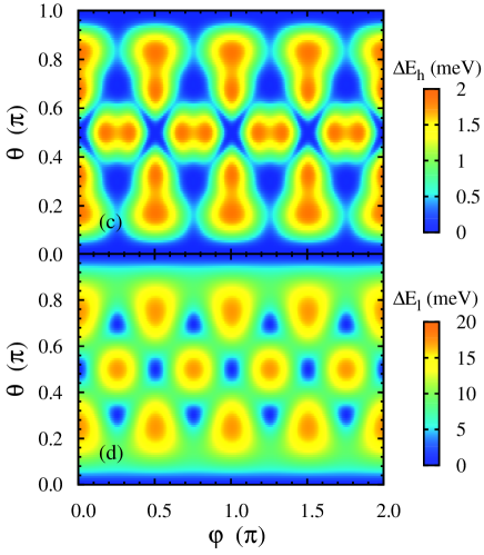
Figure 1: (Color online) (a) Energy spectra and (b) intraband splittings of the valence bands (solid curves) along the $[110]$-direction from the diagonalization of the $8\times 8$ Kane Hamiltonian. The dashed curves in (b) show the results from the $4\times 4$ Luttinger Hamiltonian. $a$ is the lattice constant. (c) and (d) show the intraband splittings of the HH and LH bands at $|{\bf k}|=0.1\pi/a$ as function of the wave direction $(\theta,\psi)$.

In this section, we present our results in bulk GaAs with the measured value of the optical deformation potential $d_{0}=48$ eV.grim ; langot The other parameterswu6 in our computation are all taken from Ref. madelung, . By numerically diagonalizing the $8\times 8$ Kane Hamiltonian, one obtains the energy spectra of the valence bands. The results along the $[110]$-direction are plotted in Fig. 1(a), where the HH, LH and split-off bands all present intraband splittings. One notices that both the HH and LH bands are approximately parabolic within $0.15$ eV from the valence-band top, which indicates the feasibility of the effective-mass approximation. Moreover, the splitting between the HH and LH bands are tens of meV even for the Fermi energy smaller than $10$ meV, corresponding to $n_{h}\approx 3\times 10^{16}$ cm^-3 at 0 K. Therefore, we neglect the interband coherence between the HH and LH bands and reduce the $4\times 4$ hole density matrices into the LH and HH blocks, both are $2\times 2$ matrices, in our computation.com_spliting In Fig. 1(b), we illustrate the intraband splittings of the three valence bands, i.e., $\Delta E_{\eta,\bf k}=E_{\eta,\bf k}^{2}-E_{\eta,\bf k}^{1}$, from the $8\times 8$ Kane Hamiltonian along the $[110]$-direction as solid curves. Here, $E_{\eta}^{2}$ ($E_{\eta}^{1}$) is the larger (smaller) eigenvalue of the $\eta$-band with $\eta$ corresponding to the HH, LH and split-off bands. One can see that the splitting of the HH band is much smaller than that of the LH band. This can be understood as follows: Within the spherical approximation, the LH band itself presents an intraband splitting due to the Dresselhaus SOC, while the HH band is still doubly degenerate as mentioned in Sec. II. However, the anisotropy property of the valence band makes the HH states contain some LH components so as to lift the degeneracy of the HH band. In other words, the SOC induces the splitting of the HH band indirectly, hence the magnitude is smaller than the direct splitting of the LH band. For comparison, we also plot the intraband splittings from the perturbation approach up to the order of $k^{3}$ based on the $4\times 4$ Luttinger Hamiltonian in Fig. 1(b) as dashed curves. One can see that the perturbation approach only performs well for $k<0.16\pi/a$. For larger wave vectors, the cubic wave-vector dependence of the intraband splitting is violated due to the interband coupling. The intraband splittings of the HH and LH bands are plotted as function of the direction of the wave vector in Fig. 1(c) and (d), respectively, from which the anisotropy properties can be clearly seen.

Since the intraband splitting is much smaller in the density and temperature regimes studied in the present work compared to the Fermi energy, one can neglect the intraband splitting in the $\delta$-function in Eqs. (15) and (16).wu4 For the numerical treatment of the scattering term, we take the isotropic energy spectrum from the effective-mass approximation, $E^{1}_{h/l,{\bf k}}\approx E^{2}_{h/l,{\bf k}}\approx E_{h/l,{\bf k}}=-\tfrac{\hbar^{2}}{2m_{0}}(\gamma_{1}\mp\bar{\gamma})k^{2}$ with $\bar{\gamma}=(\gamma_{2}+\gamma_{3})/2$.schliemann ; wu6 The feasibility of this widely adopted approximation has been shown in the literature.sliwa ; sham ; csontos Moreover, we find that the density of states from this approximation is almost the same as that obtained from the anisotropic spectrum. The average momentum scattering time in this scheme is also comparable to that from the real band structure.

III.1 HSR in intrinsic GaAs

In this part, we investigate the HSR in intrinsic case. Our discussion is based on two physical quantities, i.e., the quasi-spin polarization and the spin polarization. The former describes the population difference between the two HH and LH quasi-spin bands, defined as

$$P^{p}=\sum_{\eta\bf k}(\rho^{h}_{\eta\bf k}(1,1)-\rho^{h}_{\eta\bf k}(2,2))/n_{h},$$ (17)

with $n_{h}$ being the hole density. The latter is calculated as the spin polarization along the [001]-direction

$$P^{s}=\sum_{\eta\bf k}{\rm Tr}(\rho_{\eta\bf k}^{c}J_{z})/n_{h},$$ (18)

which reflects the optical orientation signal in experiment.

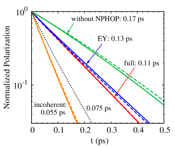
Figure 2: (Color online) Temporal evolution of the normalized quasi-spin polarization (dashed curves) and spin polarization (solid ones) at room temperature with the hole density $n_{h}=10^{17}$ cm^-3 in intrinsic GaAs. The curves labelled as “full” (“incoherent”) are obtained from the full calculation with (without) the intraband coherence, while the ones with “EY” show the results without the intraband precession term, corresponding to the contribution from the EY mechanism. The results from the calculation including the intraband coherence but without the nonpolar hole-optical-phonon scattering are plotted as the curves denoted as “without NPHOP”. The dotted curve represents the spin polarization from the calculation scheme used in Ref. krauss, , i.e., without the nonpolar hole-optical-phonon scattering and intraband coherence. The relaxation times are given correspondingly.

In our computation, we take the initial state from the optical orientation due to the pump pulse with the small polarization $P^{\rm opt}=(I^{+}-I^{-})/(I^{+}+I^{-})=2$ %,arg_p where $I^{+}$ and $I^{-}$ are the intensities of the $\sigma^{+}$- and $\sigma^{-}$-polarized light. In that case, one sets the electron density matrices as the Fermi distribution with the spin polarization 1 % at the lattice temperature and keeps it unchanged, by taking into account of the fact that the electron spin (momentum) relaxation time is much longer (shorter) than the time scale of the HSR. The initial hole density matrices are also set to obey the Fermi distribution in the collinear spin space to describe the optically excited condition. By solving the KSBEs, one obtains the temporal evolution of the spin polarization $P^{s}$ (quasi-spin one $P^{p}$), from which the spin (quasi-spin) relaxation time is extracted.

We first take the hole density $n_{h}=10^{17}$ cm^-3. Figure 2 illustrates the temporal evolution of the spin polarization (normalized by the value at $t=0$) from the full calculation at room temperature as the red solid curve (labelled as “full”). One can see that the spin polarization decays exponentially with the HSR time $\tau_{\rm tot}\approx 0.11$ ps, which agrees perfectly well with the experimental value of the HSR time, $0.11\pm$10 % ps.hilton By removing the coherent term from the KSBEs, one switches off the DP mechanism and obtains the results solely due to the EY mechanism as the blue solid curve. The HSR time $\tau_{\rm EY}$ in this case is about 0.13 ps. Since the EY mechanism is irrelevant to the spin precession, from $\tau_{\rm tot}^{-1}=\tau_{\rm EY}^{-1}+\tau_{\rm DP}^{-1}$, one extracts the spin lifetime due to the DP mechanism $\tau_{\rm DP}\approx 0.72$ ps, which is much longer than that of the EY mechanism. Therefore, the EY mechanism is dominant in this case. Moreover, we find that the relaxation time of the quasi-spin polarization (red dashed curve labelled with “full”) is very close to that of the spin polarization.

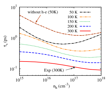
Figure 3: (Color online) HSR time from the full calculation as function of the hole density $n_{h}$ in intrinsic GaAs. The result from the calculation without the hole-electron scattering at 50 K is labeled as “without h-e”. The dot represents the experiment data at room temperature with the photo-excitation density $n_{h}=10^{17}$ cm^-3 (Ref. hilton, ). In the calculation, the electron density $n_{e}=n_{h}$.

In the figure, we also plot the results from the calculation without the intraband coherence as orange curves (labelled as “incoherent”), where the non-diagonal elements $\rho_{\eta\bf k}(1,2)$ are artificially set to be zero during the calculation as done in Ref. krauss, . Compared with the results labelled with “EY”, one immediately finds that this procedure markedly exaggerates the contribution of the EY mechanism, (The DP mechanism vanishes in this scheme obviously.) which clearly shows the problem of the missing of the intraband coherence. The reason lies in the fact that the spin-conserving scattering becomes the spin-flip one once the non-diagonal elements of the density matrices in helix representation are neglected.wu4 In Ref. krauss, , the authors argued the disregarding of the intraband coherence by arguing that the optically driven coherence between single particle states would be very small and the SOC could not drive any coherence further during the time evolution of the density matrices in the helix representation (i.e., under the basis called “intelligent basis” there). However, this is actually incorrect. Since the SOC information is transferred into the wave functions of the eigenstates in the helix representation, any spin-conserving scattering events can induce the intraband and/or interband coherence.wu4 Therefore, the same HSR time is obtained if one chooses the helix initial condition, corresponding to the initialization without any non-diagonal elements of the density matrices at $t=0$. In the remaining part of this paper, all the results are obtained from the calculation including the intraband coherence.

The green curves (labelled as “without NPHOP”) in Fig. 2 obtained from the calculation without the nonpolar hole-optical-phonon scattering give the HSR time around 0.17 ps, much longer than that from the full calculation. This clearly shows the importance of the nonpolar hole-optical-phonon scattering in the HSR. It is noted that this scattering is also missed in Ref. krauss, . For comparison, we further plot the spin polarization from the calculation without the nonpolar hole-optical-phonon scattering and the intraband coherence as black dotted curve, which corresponds to the calculation scheme in Ref. krauss, . It is seen that the missed terms have marked contribution to the HSR.

Since the direct relation between the EY mechanism and the scattering strength, the HSR time due to the EY mechanism decreases (increases) when the scattering becomes stronger (weaker). To show the influence of the scattering more clearly, we vary the density and temperature. The density dependence of the HSR time is plotted in Fig. 3. One can see that the HSR time at room temperature monotonically decreases with increasing photo-excitation density. Since the electrons and holes are both in the nondegenerate regime, the Coulomb scattering rate becomes larger as the density increases, according to the estimation of the average Coulomb scattering rate $(\tau_{p}^{C})^{-1}\propto n_{h}/T^{3/2}$.giulianni As a result, the HSR time decreases. One can also see that the HSR time markedly increases with decreasing temperature, due to the suppression of the hole-phonon scattering.

More interestingly, we predict a valley in the density dependence of the HSR time at low temperature. The minimum occurs at $n_{h}=n_{e}=4\times 10^{16}$ cm^-3 (corresponding to the Fermi temperatures $T_{F}^{e}=74$ K for electrons and $T_{F}^{h}=9$ K for holes) at $T=50$ K and $n_{h}=n_{e}=2\times 10^{17}$ cm^-3 ($T_{F}^{e}=216$ K and $T_{F}^{h}=27$ K) at $T=100$ K. The agreement between $T_{F}^{e}$ at the valley and the lattice temperature $T$ reveals that the valley results from the different density dependence of the hole-electron scattering in the degenerate and nondegenerate limits. As mentioned above, the HSR time decreases with increasing density in the nondegenerate limit. However, for high densities, electrons first enter into the degenerate regime. Therefore the hole-electron scattering strength is significantly decreased due to the Pauli-blocking of electrons. As a result, the HSR time due to the EY mechanism increases in this regime, and finally results in the valley at the crossover between the degenerate and nondegenerate regimes of electrons. In the figure, we also plot the result from the calculation without the hole-electron scattering at 50 K. It is clear to see that the valley at $n_{h}=n_{e}=4\times 10^{16}$ cm^-3 disappears, as expected. Instead, one finds that another valley shows up at $n_{h}=n_{e}=2\times 10^{17}$ cm^-3, where $T_{F}^{h}$ (27 K) is comparable to the lattice temperature $T$ (50 K). This means that holes also enter the degenerate regime at such a high density and the hole-hole scattering rate is then given by $(\tau_{p}^{C})^{-1}\propto T^{2}/n_{h}^{2/3}$.giulianni Therefore, the HSR time increases with increasing the density for $n_{h}=n_{e}>2\times 10^{17}$ cm^-3. One notices that the Coulomb scattering can also induce a peak (instead of valley) in the density dependence of the electron spin relaxation time limited by the DP mechanism, first predicted by Jiang and Wuwu6 and realized experimentally by Krauß et al..krauss2 ; shen

III.2 HSR in $p$-type GaAs

In this part, we study the HSR in $p$-type GaAs. We still apply the collinear initial spin polarization $P^{s}=2$ %. As the photo-excited carrier density is much smaller compared to the doping density, we take $n_{h}=n_{i}$ and neglect the hole-electron scattering in the computation.

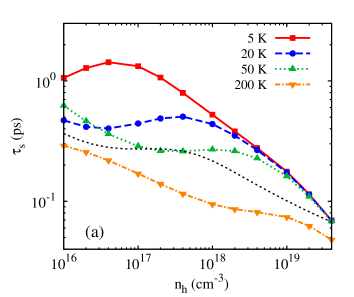
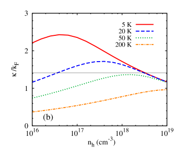
Figure 4: (Color online) (a) HSR time from the full calculation as function of the hole density $n_{h}$ in $p$-type GaAs. We take the impurity density $n_{i}=n_{h}$. The hole-impurity scattering time $\tau_{p}^{hi}$ at 20 K is plotted as the black dotted curve without symbol. (b) The ratio of the screening constant to the Fermi wave vector, $\kappa/k_{F}$, as function of the hole density. The solid line illustrates the level $\kappa=\sqrt{2}k_{F}$.

III.2.1 Density dependence

We start from the density dependence of the HSR time. The results from the full calculation are plotted in Fig. 4(a), which shows rich and intriguing nonmonotonic features. At low temperature, e.g., at 5 K, the HSR time first increases and then decreases with increasing hole density. As a result, a peak appears at $n_{h}=4\times 10^{16}$ cm^-3, where the corresponding Fermi temperature $T_{F}^{h}=9$ K is comparable to the lattice temperature. As the temperature increases, the peak moves to the higher density regime ($n_{h}=3\times 10^{17}$ cm^-3 with $T_{F}^{h}=35$ K for 20 K and $n_{h}=10^{18}$ cm^-3 with $T_{F}^{h}=79$ K for 50 K). Simultaneously, a valley gradually appears in the low density regime. Although the peak also locates at the crossover between the degenerate and nondegenerate regime, the underlying physics of the peak is again different from the one in the electron spin relaxation time in intrinsic and $n$-type materials.wu6 To explain the presence of the peak, we turn to analyze the change of the scattering strength. Since the intraband splitting is too small to affect the HSR for the hole states near the zone-center, the HSR process is mainly determined by the EY mechanism instead of the DP mechanism for low density case, especially at low temperature.

As a qualitative analysis for the case $n_{i}=n_{h}$, one can focus on the major scattering mechanism, i.e., the hole-impurity scattering with the strength estimated by $(\tau_{p}^{hi})^{-1}\sim m_{\rm eff}n_{h}\langle kV_{q}^{2}\rangle/(8\pi^{2}\hbar^{3})\propto n_{h}\langle k(q^{2}+\kappa^{2})^{-2}\rangle$, where $k$ comes from the density of states and $\langle...\rangle$ stands for the average over the distribution. $m_{\rm eff}$ represents the effective mass and $q$ is the momentum exchange. In the degenerate regime, only holes on the Fermi surface contribute to the HSR, therefore, one can estimate $k\approx k_{F}$ and $q^{2}\approx 2k_{F}^{2}$ with $k_{F}$ representing the Fermi wave vector. Thus, one has

$$\tau_{p}^{hi}\propto[2+(\kappa/k_{F})^{2}]^{2}.$$ (19)

Figure 4(b) shows the ratio of the RPA screening constant $\kappa$ to $k_{F}$. One finds that $\kappa/k_{F}$ decreases with increasing density in the high density regime and $\tau_{s}\sim\tau_{p}^{hi}$ decreases also. The density dependence of $\kappa/k_{F}$ can be easily understood once the Thomas-Fermi screening ($\kappa\propto n_{h}^{1/6}$) is applied in the degenerate limit,haug which leads to $\kappa/k_{F}\propto n_{h}^{-1/6}$.

However, the situation is quite different in the nondegenerate regime. In this limit, one has $\kappa\propto n_{h}^{1/2}T^{-1/2}$ according to the Debye-Hückel screening,haug and $q\sim k\sim T^{1/2}$. For $\kappa\gg q$, one neglects the $q^{2}$ term in $\tau_{p}^{hi}$ and obtains

$$\tau_{p}^{hi}\propto(n_{h}\langle k\kappa^{-4}\rangle)^{-1}\propto n_{h}T^{-5/2},$$ (20)

which indicates that the HSR time increases with increasing density in this case. For $\kappa\ll q$, the screening constant is neglected, and $\tau_{p}^{hi}$ can be written as

$$\tau_{p}^{hi}\propto(n_{h}\langle kq^{-4}\rangle)^{-1}\propto n_{h}^{-1}T^{3/2},$$ (21)

which decreases with increasing density. In Fig. 4(a), we also plot the density dependence of $\tau_{p}^{hi}$ at 20 K (the dotted curve without symbol), which agrees well with our discussion. It is clear to see that $\tau_{p}^{hi}$ is in the same order of magnitude as the HSR time $\tau_{s}$ as expected.

Now, the peak and valley in the HSR time in Fig. 4(a) can be well understood. For example at 20 K, holes lie in the nondegenerate regime and the screening constant is small in the low density regime. As the density increases, the HSR time decreases according to Eq. (21). Nevertheless, with further increase of the density, $\kappa$ can be larger than $q$. Then the HSR time increases with density according to Eq. (20). By further increasing density, the system enters into the degenerate regime, and the HSR time decreases again following Eq. (19). By comparing Fig. 4 (a) and (b), we find the crossover between Eqs. (20) and (21) can still be qualitatively estimated by taking $q^{2}\sim 2k_{F}^{2}$. At low temperature (5 K), the screening constant is always large in the nondegenerate regime of our investigation [see Fig. 4(b)], so the valley is invisible in Fig. 4(a). However, at high temperature (200 K), the screening is weak in both the degenerate and nondegenerate regimes and the HSR time monotonically decreases with increasing density.

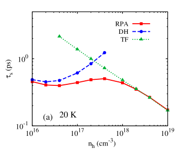
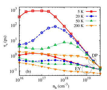
Figure 5: (Color online) (a) Density dependence of the total HSR time in $p$-type GaAs at 20 K. In the calculation, the RPA (red solid curve), Thomas-Fermi (green dotted curve) and Debye-Hückel (blue dashed curve) screenings are applied. (b) HSR times due to the EY mechanism (curves with solid symbols) and the DP mechanism (curves with open symbols) as function of the hole density.

To elucidate the role of the screening more clearly, we plot the results from different screenings at 20 K in Fig. 5(a). The green dotted and blue dashed curves correspond to the results with the Thomas-Fermi and Debye-Hückel screenings, respectively. The total HSR time from the RPA screening is also plotted as the red solid curve. One can see that the result from the RPA screening is consistent with that from the Thomas-Fermi (Debye-Hückel) screening in the high (low) density regime and the peak in the density dependence exactly occurs at the crossover between the degenerate and nondegenerate regimes.

In contrast, electrons in most $n$-type zinc-blende materials are easier to enter into the degenerate regime and the screening constant is usually small ($\kappa/k_{F}<\sqrt{2}$) thanks to the small effective mass of the conduction band. Therefore, it is difficult to observe the nonmonotonic effect of the screening during the electron spin relaxation. However, Jiang and Wu suggested that the screening from the holes in $p$-type materials can also give rise to observable effects on the electron spin relaxation.wu6 In that case, the EY mechanism is always irrelevant and the electron spin relaxation is dominated by the DP mechanism in the low hole density regime. Since the spin relaxation time due to the DP mechanism is inversely proportional to the momentum scattering time in the strong scattering limit, the hole density dependence of the electron spin relaxation time there is opposite to that of the HSR time we predict here. Specifically, they found that the electron spin relaxation time due to the DP mechanism first increases and then decreases as the hole density increases in the nondegenerate regime. After the holes enter into the degenerate regime, the electron spin relaxation time increases again.

From previous discussion, one notices that the HSR properties can be well interpreted by the EY mechanism which suggests that the EY mechanism is generally more important than the DP one. This can be clearly seen from Fig. 5(b), where the HSR times due to the EY and DP mechanisms are separately plotted. Interestingly, we find that the contribution of the DP mechanism can be comparable to that of the EY mechanism in high doping regime. To explain this behavior, we employ the relation in the strong scattering limit, $\tau_{\rm DP}\sim 1/[\langle|{\mbox{\boldmath$\Omega$\unboldmath}}|^{2}-\Omega_{z}^{2}\rangle\tau_{p}^{hi}]$ with $\langle|{\mbox{\boldmath$\Omega$\unboldmath}}|^{2}-\Omega_{z}^{2}\rangle$ representing the ensemble average of the effective magnetic field (inhomogeneous broadeningwu1 ). In the low density regime, the hole gas is in the nondegenerate limit and the inhomogeneous broadening is small and insensitive to the density. Hence the contribution of the DP mechanism to the HSR is negligible. However, holes are in the degenerate limit for high density case and the inhomogeneous broadening increases rapidly [$\propto k_{F}^{6}$, see Eq. (10) also] with increasing hole density, which makes the DP mechanism markedly contribute to the HSR. By using Eq. (19), one can easily obtain $\tau_{\rm DP}/\tau_{\rm EY}\propto n_{h}^{-2/3}$ for $\kappa/k_{F}\gg\sqrt{2}$ and $\tau_{\rm DP}/\tau_{\rm EY}\propto n_{h}^{-2}$ for $\kappa/k_{F}\ll\sqrt{2}$. It is obvious that $\tau_{\rm DP}/\tau_{\rm EY}$ decreases with increasing density in both cases.

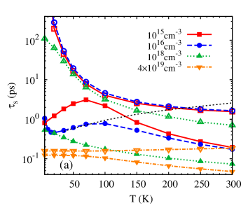
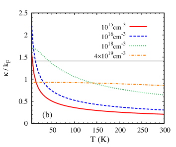
Figure 6: (Color online) (a) HSR times due to the EY (curves with solid symbols) and DP (curves with open symbols) mechanisms as function of the temperature in $p$-type GaAs with $n_{i}=n_{h}$. The result without the hole-phonon scattering at $n_{h}=10^{16}$ cm^-3 is plotted as dotted curve without symbol. (b) The ratio of the screening constant to the Fermi wave vector as function of the temperature. The level $\kappa=\sqrt{2}k_{F}$ is illustrated by a solid line.

III.2.2 Temperature dependence

Similarly, one also finds the nonmonotonic temperature dependence of the HSR time. In Fig. 6(a), we plot the results of four typical densities $n_{h}=10^{15}$, $10^{16}$, $10^{18}$ and $4\times 10^{19}$ cm^-3. One notices that the temperature dependence of the HSR time is also qualitatively determined by the EY mechanism (curves with solid symbols). The HSR time from this mechanism first decreases and then increases with increasing temperature for $n_{h}=10^{16}$ cm^-3, and the minimum reaches around 15 K. Since the hole-phonon scattering is rather weak in this regime, this feature just reflects the important role of the screening in the hole-impurity scattering. Figure 6(b) illustrates the ratio of the screening constant to the Fermi wave vector, where the crossover ($\kappa\approx\sqrt{2}k_{F}$) occurs just around 15 K. Since holes are always nondegenerate in this case (even at 5 K, see Fig. 4), the HSR time decreases (increases) with increasing temperature below (above) 15 K, according to Eq. (20) [Eq. (21)]. Moreover, we find that the HSR time decreases again when the temperature further increases, because of the enhancement of the hole-phonon scattering. To demonstrate this picture, we remove the hole-phonon scattering from the KSBEs and find that the HSR time due to the EY mechanism monotonically increases above 15 K, as expected (shown as dotted curve without symbol). For $n_{h}=10^{15}$ cm^-3, only the peak is visible while the valley is absent as the curve with solid squares shown. The reason is that the screening is weak for this density [see Fig. 6(b)]. However, for $n_{h}=10^{18}$ and $4\times 10^{19}$ cm^-3, holes are in the degenerate regime at low temperature, hence the temperature dependence of the HSR time is determined by $\kappa/k_{F}$ from Eq. (19). At high temperature regime, the HSR time is also limited by the hole-phonon scattering for these densities. Another important information one can get from Fig. 6(a) is that the HSR time due to the DP mechanism is comparable to the one due to the EY mechanism around 80 K for $n_{h}=10^{15}$ cm^-3. For the high doping case with $n_{h}=4\times 10^{19}$ cm^-3, the important role of the DP mechanism at low temperature can also be clearly seen [see also Fig. 5(b)].

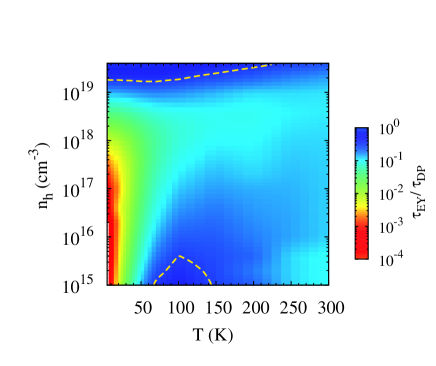
Figure 7: (Color online) Ratio of the HSR time due to the EY mechanism to that due to the DP mechanism, $\tau_{\rm EY}/\tau_{\rm DP}$, as function of the doping density and temperature in $p$-type GaAs with $n_{i}=n_{h}$. The yellow dashed curves represent the borders with $\tau_{\rm EY}/\tau_{\rm DP}=1/3$

III.2.3 Relative contribution of the DP and EY mechanisms

For thorough understanding of the relative contribution of the DP and EY mechanisms, we plot the ratio of the HSR times due to the EY and DP mechanisms $\tau_{\rm EY}/\tau_{\rm DP}$ as function of the density and temperature in Fig. 7. It is clear to see that the HSR time is dominated by the EY mechanism at low temperature (below 40 K) upto $10^{19}$ cm^-3. This is because that holes mainly occupy the states with small wave vectors and experience a small effective Dresselhaus field. In the high density regime, the increase of the inhomogeneous broadening makes the DP contribution significantly enhanced and even comparable to the EY one as discussed above. Another interesting regime lies in the low density regime at moderate temperature, where the contribution of the DP mechanism can also be comparable to that of the EY mechanism. This originates from the reduction of the EY contribution due to the relatively weak hole-impurity scattering according to Eq. (21) [see Fig. 6(a) also]. However, this effect is suppressed by the hole-phonon scattering at higher temperature, where the EY mechanism again is more efficient than the DP one. In the figure, we also plot the borders with $\tau_{\rm EY}/\tau_{\rm DP}=1/3$ as yellow dashed curves.

Finally, we should point out that the Bir-Aronov-Pikus mechanismBAP is neglected in our computation even in the intrinsic case. The reason lies in the fact that the spin-flip process due to the electron-hole exchange interaction in intrinsic GaAs occurs in the time scale of nanosecond,wu6 therefore this mechanism is irrelevant to the ultrafast spin relaxation of the hole system.

IV Conclusion

In conclusion, we have investigated the HSR from the fully microscopic KSBEs in intrinsic and $p$-type bulk GaAs. We analyze the valence-band structure by considering the anisotropic property and the Dresselhaus spin-orbit coupling. We find that the degeneracy of the HH band and that of the LH band are both lifted by intraband splittings. The DP mechanism associated with the intraband precessions and the EY mechanism due to the direct spin-flip scattering are then explicitly studied, with the intraband coherence included. Our result of intrinsic GaAs shows good agreement with the experiment data at room temperature, where the EY mechanism is demonstrated to be the dominant spin relaxation mechanism due to the strong scattering process. We also show that the approach without the intraband coherence used in the literature is inadequate in accounting for the HSR and the nonpolar hole-optical-phonon, missed in the previous theoretical work, is important to the HSR. The temperature can markedly affect the HSR time by changing the strength of the hole-phonon scattering. At low temperature, we predict a valley due to the Coulomb scattering in the HSR time at the crossover between the degenerate and the nondegenerate regimes of the electrons. In $p$-type GaAs, we find that the HSR time depends on density and temperature nonmonotonically. For the density dependence, the HSR time presents a peak at the crossover between the degenerate and nondegenerate regimes of the holes, resulting from the different features of the screening in the degenerate and nondegenerate limits. In the nondegenerate regime, we predict a valley, from the competition between the screening constant and the momentum exchange, in the density dependence of the HSR time. We also find that the HSR time monotonically decreases with increasing density at high temperature, thanks to the small screening constant. For the temperature dependence, we predict a valley in the low temperature regime, which also reflects the role of the screening. In the high temperature regime, the hole-phonon scattering can markedly contribute to the HSR and make the HSR time decrease with increasing temperature. Moreover, we find that the contribution of the DP mechanism can be comparable with that of the EY one in the high density regime at low temperature and in the low density regime at moderate temperature, even though the EY mechanism is usually the major mechanism in the HSR.

Appendix A Detail of intraband splitting

The coefficients in Eq. (8) can be expressed as

$$a_{1}^{h/l} = (E^{h/l}-G)/[{(E^{h/l}-G)^{2}+|H|^{2}+|I|^{2}}]^{\frac{1}{2}},$$ (22)

$$b_{1}^{h/l} = H^{\ast}/[(E^{h/l}-G)^{2}+|H|^{2}+|I|^{2}]^{\frac{1}{2}},$$ (23)

$$c_{1}^{h/l} = I^{\ast}/[(E^{h/l}-G)^{2}+|H|^{2}+|I|^{2}]^{\frac{1}{2}},$$ (24)

and those in Eq. (9) are given by $a_{2}^{h/l}=a_{1}^{h/l}$, $b_{2}^{h/l}=-(b_{1}^{h/l})^{\ast}$ and $c_{2}^{h/l}=(c_{1}^{h/l})^{\ast}$.

The effective magnetic field in Eq. (10) can be written as

$$\Omega^{e}_{x} = h_{x}{\rm Re}(\sqrt{3}a_{2}c_{2}-b_{2}^{2}+c_{2}^{2})-h_{z}{\rm Re}(b_{2}c_{2})$$ (25)

$$\mbox{}+h_{y}{\rm Im}(\sqrt{3}a_{2}c_{2}-b_{2}^{2}-c_{2}^{2}),$$

$$\Omega^{e}_{y} = -h_{x}{\rm Im}(\sqrt{3}a_{2}c_{2}-b_{2}^{2}+c_{2}^{2})+h_{z}{\rm Im}(b_{2}c_{2})$$ (26)

$$\mbox{}+h_{y}{\rm Re}(\sqrt{3}a_{2}c_{2}-b_{2}^{2}-c_{2}^{2}),$$

$$\Omega^{e}_{z} = h_{x}{\rm Re}(\sqrt{3}a_{2}b_{1}+2b_{1}c_{2})+h_{y}{\rm Im}(\sqrt{3}a_{1}b_{1}-2b_{2}c_{1})$$ (27)

$$\mbox{}+h_{z}(3a_{1}^{2}+|b_{1}|^{2}-|c_{1}|^{2})/2,$$

where the labels “$h/l$” are neglected for short.

Appendix B Deformation potential matrix of optical phonons

The $6\times 6$ deformation potential matrix of optical phonons for valence bands readsscholz

$${\bar{D}}_{\lambda{\bf q}}=\frac{d_{0}}{a}\left(\begin{array}[]{cc}T_{\lambda\bf q}&P^{\dagger}_{\lambda\bf q}\\ P_{\lambda\bf q}&0_{2\times 2}\end{array}\right),$$ (28)

with

$$T_{\lambda\bf q} = \left(\begin{array}[]{cccc}0&\delta_{\lambda}^{+}&i\delta_{\lambda}^{z}&0\\ \delta_{\lambda}^{-}&0&0&i\delta_{\lambda}^{z}\\ -i\delta_{\lambda}^{z}&0&0&-\delta_{\lambda}^{+}\\ 0&-i\delta_{\lambda}^{z}&-\delta_{\lambda}^{-}&0\end{array}\right),$$ (33)

$$P_{\lambda\bf q} = \left(\begin{array}[]{cccc}-i\sqrt{\tfrac{1}{2}}\delta_{\lambda}^{-}&0&i\sqrt{\tfrac{3}{2}}\delta_{\lambda}^{+}&-\sqrt{2}\delta_{\lambda}^{z}\\ \sqrt{2}\delta_{\lambda}^{z}&-i\sqrt{\tfrac{3}{2}}\delta_{\lambda}^{-}&0&i\sqrt{\tfrac{1}{2}}\delta_{\lambda}^{+}\end{array}\right),$$ (36)

where $\delta_{\lambda}^{\pm}=\delta_{\lambda x}\pm i\delta_{\lambda y}$ and $\delta_{\lambda}^{z}=\delta_{\lambda z}$. $d_{0}$ and $a$ are optical deformation potential and lattice constant, respectively.

References

- (1) F. Meier and B. P. Zakharchenya, Optical Orientation (North-Holland, Amsterdam, 1984).
- (2) S. A. Wolf, D. D. Awschalom, R. A. Buhrman, J. M. Daughton, S. Von Molnár, M. L. Roukes, A. Y. Chtchelkanova, and D. M. Treger, Science 294, 1488 (2001).
- (3) Semiconductor Spintronics and Quantum Computation, edited by D. D. Awschalom, D. Loss and N. Samarth (Springer-Verlag, Berlin, 2002); I. Z̆utić, J. Fabian, and S. Das Sarma, Rev. Mod. Phys. 76, 323 (2004); J. Fabian, A. Matos-Abiague, C. Ertler, P. Stano, and I. Z̆utić, Acta Phys. Slov. 57, 565 (2007); Spin Physics in Semiconductors, edited by M. I. D’yakonov (Springer, Berlin, 2008); and references therein.
- (4) T. Korn, Phys. Rep., doi:10.1016/j.physrep.2010.05.001 (2010); and references therein.
- (5) M. W. Wu, J. H. Jiang, and M. Q. Weng, Phys. Rep. 493, 61 (2010); and references therein.
- (6) Z. G. Chen, S. G. Carter, R. Bratschitsch, and S. T. Cundiff, Physica E 42, 1803 (2010).
- (7) M. M. Glazov, E. Ya. Sherman, and V. K. Dugaev, Physica E 42, 2157 (2010).
- (8) R. J. Seymour, M. R. Junnarkar, and R. R. Alfano, Phys. Rev. B 24, 3623 (1981).
- (9) K. Zerrouati, F. Fabre, G. Bacquet, J. Bandet, J. Frandon, G. Lampel, and D. Paget, Phys. Rev. B 37, 1334 (1998).
- (10) J. M. Kikkawa and D. D. Awschalom, Phys. Rev. Lett. 80, 4313 (1998).
- (11) P. H. Song and K. W. Kim, Phys. Rev. B 66, 035207 (2002).
- (12) L. H. Teng, P. Zhang, T. S. Lai, and M. W. Wu, Europhys. Lett. 84, 27006 (2008).
- (13) S. Oertel, J. Hübner, and M. Oestreich, Appl. Phys. Lett. 93, 132112 (2008).
- (14) J. H. Jiang and M. W. Wu, Phys. Rev. B 79, 125206 (2009).
- (15) M. Römer, H. Bernien, G. Müller, D. Schuh, J. Hübner, and M. Oestreich, Phys. Rev. B 81, 075216 (2010).
- (16) M. Krauß, H. C. Schneider, R. Bratschitsch, Z. Chen, and S. T. Cundiff, Phys. Rev. B. 81, 035213 (2010).
- (17) K. Shen, Chin. Phys. Lett. 26, 067201 (2009).
- (18) D. J. Hilton and C. L. Tang, Phys. Rev. Lett. 89, 146601 (2002).
- (19) D. Culcer, C. Lechner, and R. Winkler, Phys. Rev. Lett. 97, 106601 (2006).
- (20) Z. G. Yu, S. Krishnamurthy, M. van Schilfgaarde, and N. Newman, Phys. Rev. B 71, 245312 (2005).
- (21) Y. Yafet, Phys. Rev. 85, 478 (1952); R. J. Elliott, ibid. 96, 266 (1954).
- (22) M. I. D’yakonov and V. I. Perel’, Zh. Eksp. Teor. Fiz. 60, 1954 (1971) [Sov. Phys. JETP 33, 1053 (1971)].
- (23) M. W. Wu and C. Z. Ning, Eur. Phys. J. B 18, 373 (2000); M. W. Wu, J. Phys. Soc. Jpn. 70, 2195 (2001).
- (24) M. Q. Weng and M. W. Wu, Phys. Rev. B 68, 075312 (2003).
- (25) M. M. Glazov and E. L. Ivchenko, Pis’ma Zh. Eksp. Teor. Fiz. 75, 476 (2002) [JETP Lett. 75, 403 (2002)].
- (26) M. Krauß, M. Aeschlimann, and H. C. Schneider, Phys. Rev. Lett. 100, 256601 (2008).
- (27) R. Scholz, J. Appl. Phys. 77, 3219 (1995).
- (28) P. Langot, R. Tommasi, and F. Vallée 54, 1775 (1996).
- (29) T. Brudevoll, T. A. Fjeldy, J. Baek, and M. S. Shur, J. Appl. Phys. 67, 7373 (1990).
- (30) C. Lü, U. Zülicke, and M. W. Wu, Phys. Rev. B 78, 165321 (2008).
- (31) C. Lü, J. L. Cheng, and M. W. Wu, Phys. Rev. B 73, 125314 (2006).
- (32) J. M. Luttinger, Phys. Rev. 102, 1030 (1956).
- (33) G. Dresselhaus, Phys. Rev. 100, 580 (1955).
- (34) R. Winkler, Spin-Orbit Coupling Effects in Two-Dimensional Electron and Hole Systems (Springer, Berlin, 2003).
- (35) C. Y. P. Chao and S. L. Chuang, Phys. Rev. B 46, 4110 (1992).
- (36) G. Dresselhaus, A. F. Kip, and C. Kittel, Phys. Rev. 98, 368 (1955).
- (37) P. O. Löwdin, J. Chem. Phys. 19, 1396 (1951).
- (38) A. Baldereschi and N. O. Lipari, Phys. Rev. B 8, 2697 (1973).
- (39) J. Schliemann, Phys. Rev. B 74, 045214 (2006).
- (40) E. O. Kane, J. Phys. Chem. Solids 1, 249 (1957).
- (41) J. L. Cheng and M. W. Wu, J. Appl. Phys. 99, 083704 (2006).
- (42) J. Zhou, J. L. Cheng, and M. W. Wu, Phys. Rev. B 75, 045305 (2007).
- (43) M. H. Grimsditch, D. Olego, and M. Cardona, Phys. Rev. B 20, 1758 (1979).
- (44) Semiconductors, edited by O. Madelung (Springer-Verlag, Berlin, 1987), Vol. 17a.
- (45) C. Śliwa and T. Dietl, Phys. Rev. B 74, 245215 (2006).
- (46) L. Cywiński and L. J. Sham, Phys. Rev. B 76, 045205 (2007).
- (47) D. Csontos, P. Brusheim, U. Zülicke, and H. Q. Xu, Phys. Rev. B 79, 155323 (2009).
- (48) In the small polarization case, the HSR time is insensitive to the polarization according to our computation.wu
- (49) Even in the lowest density and temperature limit in our computation, i.e., cm3 and K, the spin relaxation are mainly determined by the heavy holes with energies around 1.5 meV. The interband splitting there is about 10 meV, much larger than meV. Therefore, it is still reasonable to treat the LH and HH separately.
- (50) G. F. Giulianni and G. Vignale, Quantum Theory of the Electron Liquid (Cambridge University Press, Cambridge, England, 2005).
- (51) H. Haug and S. W. Koch, Quantum Theory of the Optical and Electronic Properties of Semiconductors, 4th ed. (World Scientific, Singapore, 2004).
- (52) G. L. Bir, A. G. Aronov, and G. E. Pikus, Zh. Eksp. Teor. Fiz. 69, 1382 (1975) [Sov. Phys. JETP 42, 705 (1976)].