Antisymmetric field in string gas cosmology

Abstract

We study how the introduction of a 2-form field flux modify the dynamics of a T-duality invariant string gas cosmology model of Greene, Kabat and Marnerides. It induces a repulsive potential term in the effective action for the scale factor of the spacial dimensions. Without the 2-form field flux, the universe fails to expand when the pressure due to string modes vanishes. With the presence of a homogeneous 2-form field flux, it propels 3 spacial dimensions to grow into a macroscopic 4 dimensional space-time. We find that it triggers an expansion of a universe away from the oscillating phase around the self-dual radius. We also investigate the effects of a constant 2-form field. We can obtain an expanding 4 dimensional space-time by tuning it at the critical value.

June 2010

1 Introduction

Since it was first proposed by Brandenberger and Vafa [1, 2, 3, 4], the string gas cosmology scenario has generated a significant amount of interest. One of its most appealing characteristics is that it provides a mechanism for dynamically generating a four dimensional space-time. This argument is based on the assumption that strings interact mainly by intersecting each other. If that is the case, the probability of intersection in space-time of two worldsheets has non-zero measure only if the dimension is equal or less than 4. This is a classical argument and it is not obvious that it will remain true if quantum effects are taken into account. There have been several attempts at trying to formulate and prove the Brandenberger-Vafa mechanism with mixed results [5, 6, 7, 8, 9]. A recent work [10], for example, succeeds in decompactifying 3 large spacial dimensions for a gas of diluted strings.

Apart from the Brandenberger-Vafa mechanism, there have been other attempts to produce a mechanism for realizing a four dimensional space-time [11, 12]. One of these scenarios consists in the inclusion of a two-form field. This field is already present in the supergravity action, hence, it is natural to consider its appearance in the equations of motion. Cosmologies with a two-form field had been studied in the past and several solutions are known [13]. In the context of string gas cosmology, a two-form field flux was introduced for dilaton-gravity in [14, 15]. In these solutions the 2-form field flux is restricted to a 4-dimensional submanifold of space-time. The two-form field flux introduces a repulsive potential in the equations of motion for the scale factor of the spacial dimensions. As a result the expansion of three spacial dimensions is enhanced and the corresponding scale factors become large.

In [16], Greene et al. introduced a higher derivative dilaton gravity model. This model replaces the Newtonian-like kinetic terms in the dilaton gravity action by their relativistic counterparts. By doing this, one obtains a model with some nice features: derivatives with respect to the cosmic time become bounded, singularities at finite time are avoided, bounces on the scale factor are produced and loitering phases that solve the horizon problem are realized. Since this model respects T-duality, it has been applied to investigate stringy cosmology such as the Brandenberger-Vafa scenario. The results has shown that this model could lead to a 4 dimensional space-time only with a fine tuning. In general 3 large spacial dimensions are not preferred and any number of dimensions could become large.

Because of the many appealing features of this model, it is interesting to investigate its behavior in the presence of an antisymmetric tensor field. The effects of such kind of field have been studied in several works [13, 17] in the context of dilaton gravity. There have been some studies also for the string gas cosmology [14, 15] case. For string gas cosmology, it is specially interesting to introduce a 2-form gauge field. Since the initial configuration is supposed to be compactified on a $d$-dimensional torus, there exist non-trivial effects even for a constant gauge field as strings can wrap the compact dimensions.

In section 2, we briefly recall the low-energy string effective action. In section 3, we introduce a T-duality invariant effective action with 2-form field flux. We obtain analytic solutions of the effective action in several limiting cases. We find they can explain qualitative behaviors of the numerical solutions. One of the main features of the string cosmology model is the introduction of a Hagedorn phase for the early universe. It arguably removes the initial singularity of the universe. We find that a homogeneous 2-form field flux triggers an expansion of a universe away from the oscillating phase around the self-dual radius. An interesting stringy effect, as explained in section 4, is that an electric like two-form field modifies the effective string tension and the Hagedorn temperature [18, 19]. In such a case, the energy of the winding modes can vanish for the directions parallel to the electric field. We find that these spacial directions can expand even if the winding modes are present. We conclude in section 5.

2 Low-energy string effective action

In this section we recall the low energy effective action for string theory.

The low energy effective action in the string frame is given by [20]

$$S=\frac{1}{2\kappa_{10}^{2}}\int d^{10}x\sqrt{-g}e^{-\phi}\left(R+(\nabla\phi)^{2}-V-\frac{1}{12}H^{2}\right)+\int d^{10}x\sqrt{-g}\mathcal{L}_{matter}$$ (2.1)

where $\kappa_{10}^{2}=8\pi G_{10}$ and $H^{2}=H_{\mu\nu\lambda}H^{\mu\nu\lambda}$ with $H_{\mu\nu\lambda}=\partial_{[\mu}B_{\nu\lambda]}$. The sign convention is all $+$ according to the classification in Misner, Thorne and Wheeler [21]. The variation of this action gives the equations of motion

$$R_{\mu}^{\nu}-\frac{1}{2}g^{\nu}_{\mu}R=\kappa_{10}^{2}e^{\phi}T_{\mu}^{\nu}+\frac{1}{12}(3H_{\mu\lambda\kappa}H^{\nu\lambda\kappa}-\frac{1}{2}g^{\nu}_{\mu}H^{2})-\frac{1}{2}g_{\mu}^{\nu}V$$

$$~{}~{}~{}~{}~{}~{}~{}~{}~{}~{}~{}~{}~{}~{}~{}~{}~{}~{}-\frac{1}{2}g_{\mu}^{\nu}(\nabla\phi)^{2}+(g_{\mu}^{\nu}g^{\lambda\kappa}-g_{\mu}^{\lambda}g^{\nu\kappa})\nabla_{\lambda}\nabla_{\kappa}\phi$$ (2.2)

$$\nabla_{\mu}(e^{-\phi}H^{\mu\nu\lambda})=0$$ (2.3)

$$2\Box\phi+R-(\nabla\phi)^{2}-V-\frac{1}{12}H^{2}=0$$ (2.4)

where $T_{\mu\nu}$ is the energy-momentum tensor derived from the matter Lagrangian. We assume the space-time metric is of the following type in the string frame

$$ds^{2}=-dt^{2}+a^{2}dx_{i}dx^{i}+b^{2}dx_{I}dx^{I}~{},~{}~{}~{}i=\{1,2,3\}~{},~{}I=\{4,...,9\}$$ (2.5)

with

$$a\equiv e^{\lambda(t)}~{},\quad b\equiv e^{\nu(t)}$$ (2.6)

By a conformal rescaling

$${\tilde{g}}_{\mu\nu}=e^{-\frac{\phi}{4}}g_{\mu\nu}$$ (2.7)

we obtain the effective action in the Einstein frame

$$S = \frac{1}{2\kappa_{10}^{2}}\int d^{10}x~{}\sqrt{-\tilde{g}}\left(\tilde{R}-\frac{1}{8}(\tilde{\nabla}_{\mu}\phi)^{2}-V\text{e}^{\frac{\phi}{4}}-\frac{1}{12}\text{e}^{-\frac{\phi}{2}}\tilde{H}^{2}\right)$$ (2.8)

$$+\int d^{10}~{}x\sqrt{-\tilde{g}}~{}\text{e}^{-\frac{5\phi}{4}}\mathcal{L}_{matter}$$

The field equations are

$$\tilde{R}_{\mu\nu}-\frac{1}{2}\tilde{g}_{\mu\nu}\tilde{R}=\kappa_{10}^{2}(\tilde{T}_{\mu\nu}+{}^{(H)}\tilde{T}_{\mu\nu}+{}^{(\phi)}\tilde{T}_{\mu\nu}+{}^{(V)}\tilde{T}_{\mu\nu})$$ (2.9)

$$\tilde{\nabla}_{\mu}(e^{-\frac{\phi}{2}}\tilde{H}^{\mu\nu\lambda})=0$$ (2.10)

$$\tilde{\Box}\phi-Ve^{\frac{\phi}{4}}+\frac{1}{6}e^{-\frac{\phi}{4}}\tilde{H}^{2}=0$$ (2.11)

The homogeneous metric is given by

$$d\tilde{s}^{2}=-d\tilde{t}^{2}+\tilde{a}^{2}dx_{i}dx^{i}+\tilde{b}^{2}dx_{I}dx^{I}~{},~{}~{}~{}i=\{1,2,3\}~{},~{}I=\{4,...,9\}$$ (2.12)

with

$$\tilde{a}\equiv e^{\alpha(\tilde{t})}~{},\quad\tilde{b}\equiv e^{\beta(\tilde{t})}~{}$$ (2.13)

More detailed relations between the string frame and the Einstein frame are explained in the appendix A.

We need a nontrivial solution for the field strength $H_{\mu\nu\lambda}$ to investigate its effects on the cosmology. The equation of motion for the two-form field (2.10) can be solved using the Freund-Rubin ansatz [22]

$$H^{\mu\nu\alpha}=e^{\phi}\epsilon^{\mu\nu\alpha\beta}\nabla_{\beta}h~{},~{}\text{with}~{}~{}\epsilon^{\mu\nu\lambda\kappa}=\frac{4!}{\sqrt{-g}}\delta^{\mu}_{[0}\delta^{\nu}_{1}\delta^{\lambda}_{2}\delta^{\kappa}_{3]}$$ (2.14)

We assume here that the two-form field flux exists only in three spacial directions. This assumption is consistent with the symmetry of the postulated space-time metric. Because $\nabla^{\mu}\epsilon_{\mu\nu\alpha\beta}=0$, the equation of motion is automatically satisfied. It only remains to satisfy the closure condition [13]

$$\nabla_{[\beta}H_{\mu\nu\alpha]}=0$$ (2.15)

The equation of motion is then

$$\sum_{\mu,\nu=0}^{3}g^{\mu\nu}\partial_{\mu}(a^{3}b^{-6}e^{\phi}h,_{\nu})=0$$ (2.16)

In the case of a homogeneous field $h\equiv h(t)$, we obtain

$${\ddot{h}}+(3\dot{\lambda}-6\dot{\nu}+\dot{\phi}){\dot{h}}=0~{}~{}~{}~{}~{}$$ (2.17)

with $H_{o}$ a positive constant and $\dot{}\equiv\frac{d}{dt}$. This equation is solved by

$$\dot{h}=\frac{\pm H_{0}{b}^{6}}{{a}^{3}}e^{-\phi}$$ (2.18)

Thus, we have for these $H_{\mu\nu\lambda}$

$$H_{\mu\lambda\kappa}H^{\nu\lambda\kappa} = 0~{}~{}\text{if}~{}~{}\mu~{},\nu=\{0,4,5,...,9\}$$ (2.19)

$$H_{i\lambda\kappa}H^{j\lambda\kappa} = \frac{2H_{o}^{2}}{a^{6}}\delta^{j}_{i}~{}~{}\text{for}~{}~{}i,~{}j=\{1,2,3\}$$ (2.20)

In particular we have $H^{2}=6H_{o}^{2}a^{-6}$.

As in [1, 5, 14, 16] we consider a very simple setup with 3 types of matter: isotropic winding modes (with all winding numbers $W_{i}=W,~{}i=\{1,2,3\}$) with energies

$$E_{W}=6We^{\lambda}~{}$$ (2.21)

isotropic momentum modes (with all momenta $K_{i}=K,~{}i=\{1,2,3\}$) with energies

$$E_{K}=6Ke^{-\lambda}$$ (2.22)

and string oscillator modes that are modeled as pressureless dust with energy $E_{\text{dust}}$ . The total energy is the sum

$$E=E_{W}+E_{K}+E_{\text{dust}}+V$$ (2.23)

with $V=V(\varphi)$ the potential for the dilaton. In an adiabatic system the pressures are

$$P_{\varphi} = \frac{\partial E}{\partial\varphi}=\frac{\partial F}{\partial\varphi}=-\frac{\partial L_{\text{m}}}{\partial\varphi}=\frac{\partial V}{\partial\varphi}~{}$$ (2.24)

$$P_{\lambda} = -\frac{1}{3}\frac{\partial F}{\partial\lambda}=-\frac{1}{3}\frac{\partial L_{\text{m}}}{\partial\lambda}=-\frac{1}{3}\frac{\partial E}{\partial\lambda}=2Ke^{-\lambda}-2We^{\lambda}~{}$$ (2.25)

The energy of the string gas is defined as $E_{s}\equiv E_{W}+E_{K}+E_{\text{dust}}$.

In order to model the behavior of the gas, we consider the following phases as in [16]:

• Hagedorn phase: thermal equilibrium at temperature $T_{H}=1/(\sqrt{8}\pi)$. The free energy of the gas vanishes ($P_{\lambda}=0$) and $E_{s}$ is conserved

  $$\langle W\rangle=\frac{\sqrt{E_{s}}}{12\sqrt{\pi}}e^{-\lambda}\quad,\quad\langle K\rangle=\frac{\sqrt{E_{s}}}{12\sqrt{\pi}}e^{\lambda}$$ (2.26)

• Radiation phase: thermal equilibrium at $T<T_{H}$ with the universe dominated by massless string modes. In $d+1$ dimensional space-time, the internal energy is

  $$E_{s}=c_{d}V_{d}T^{d+1},\qquad c_{d}=128\frac{2d!\zeta(d+1)}{(4\pi)^{d/2}\gamma(d/2)}(2-2^{-d})$$ (2.27)

  with $V_{d}=(2\pi)^{d}e^{d|\lambda|}$: the T-duality invariant volume.

  $$F=E_{s}-TS=-\frac{1}{d}c_{d}V_{d}T^{d+1}$$ (2.28)

  $$P_{\lambda}=\text{sign}(\lambda)E_{s}/d$$ (2.29)

  $$\lambda>0: \langle W\rangle=0\quad,\quad\langle K\rangle=\frac{1}{2}P_{\lambda}e^{\lambda}\quad\text{(radiation phase)}$$ (2.30)

  $$\lambda<0: \langle W\rangle=-\frac{1}{2}P_{\lambda}e^{-\lambda}\quad,\quad\langle K\rangle=0\quad\text{(winding mode dominated phase)}$$ (2.31)

  Note that the radiation and winding mode dominated phases are T-dual to each other.

• Frozen phase: in this phase the interactions between strings are turned off. The momentum and winding numbers are conserved, so $K$ and $W$ are frozen at the values they have on Hagedorn exit.

• Non-equilibrium phase: In order to model the string gas, we consider a phase in which the the temperature falls below the Hagedorn temperature. Since we also consider the interactions among the strings, the expectation value of the momenta and winding number deviate from their equilibrium values such that the pressure of the string gas does not vanish.

3 T-duality invariant action with two-form field

In order to analyze the effect of the two-form field, we work in the string frame. This allow us to choose a solution where the scale factor $\nu$, defined in (2.6), becomes constant and the analysis can be restricted to a 4-dimensional cosmology in the presence of a two-form field.

In the case of a homogeneous space-time [14, 15, 17], the action (2.1) can be reduced to

$$S=\int dt\big{[}4\pi e^{-\varphi}(d\dot{\lambda}^{2}-\dot{\varphi}^{2}-U_{0}(\lambda))+L_{m}\big{]}~{}$$ (3.1)

with $L_{m}$: the matter lagrangian, $\varphi$: related to the original dilaton $\phi$ as $\varphi=2\phi-d\lambda~{}.$ The potential $U(\lambda)$ arises due to the nontrivial two-form field strength $H_{\mu\nu\lambda}$, as shown in [13, 14]

$$H^{2}_{\mu\nu\alpha}=12H_{0}^{2}e^{-2d\lambda}\equiv 24U_{0}(\lambda)~{}$$ (3.2)

The parameter $d$ counts the number of spacial dimensions with the homogeneous scale factor $\lambda$. Although our case corresponds to $d=3$ such that the space-time is 4-dimensional, we retain $d$ dependence explicitly in the equations of motion in order to keep track of the algebra.

Now we proceed as [16] and replace the canonical kinetic terms by their higher derivative extensions. This leads to a phenomenological action with bounded velocities $\dot{\varphi}$, $\dot{\lambda}$. It thus rules out singularities at any finite proper time. With this modification we obtain a higher derivative action for the dilaton and scale factor which are coupled to a two-form field strength

$$S=\int dt\Big{[}8\pi e^{-\varphi}\Big{(}\sqrt{1-\dot{\varphi}^{2}}-\sqrt{1-d\dot{\lambda}^{2}}-U(\lambda)\Big{)}+L_{m}\Big{]}~{}$$ (3.3)

$L_{m}=-F$ is the negative of the matter free energy (of the string gas) and $U(\lambda)$ is a modified potential as explained below.

String gas cosmology model needs to respect T-duality, a fundamental symmetry in string theory originating from the existence of the minimal length (string scale). It is realized as the symmetry between the winding and momentum modes in a toroidal compactification. Since (3.2) is not explicitly invariant under T-duality, it is necessary to modify this potential in order to realize the symmetry. Such a modification allows us to solve the equations of motion near the self-dual radius numerically. An adequate choice is

$$U(\lambda)\equiv\frac{1}{2}H_{0}^{2}(e^{2\lambda}+e^{-2\lambda})^{-d}=\frac{1}{2^{d+1}}H_{0}^{2}(\cosh 2\lambda)^{-d}~{}$$ (3.4)

as (3.4) is not singular at $\lambda=0$ and it reduces to (3.2) for large $\lambda$.

Defining the relativistic factors [16]

$$\gamma_{\varphi}\equiv\frac{1}{\sqrt{1-\dot{\varphi}^{2}}}~{},~{}~{}~{}~{}\gamma_{\lambda}\equiv\frac{1}{\sqrt{1-d\dot{\lambda}^{2}}}~{}$$ (3.5)

the equations of motion obtained from the action (3.3) are

$$\dot{\gamma}_{\varphi} = \dot{\varphi}(\gamma_{\varphi}-\gamma_{\lambda}^{-1}-U(\lambda))+\frac{1}{8\pi^{2}}\dot{\varphi}e^{\varphi}P_{\varphi}~{}$$ (3.6)

$$\dot{\gamma}_{\lambda} = \dot{\varphi}(\gamma_{\lambda}-\gamma_{\lambda}^{-1})-\dot{\lambda}\frac{\partial U}{\partial\lambda}+\frac{1}{8\pi^{2}}d\dot{\lambda}e^{\varphi}P_{\lambda}~{}$$ (3.7)

We also need to impose the Hamiltonian constraint

$$\gamma_{\varphi}-\gamma_{\lambda}-U(\lambda)=\frac{1}{8\pi^{2}}Ee^{\varphi}~{}$$ (3.8)

where $E$ is the energy contained in matter. Notice that in the positive energy region $\gamma_{\varphi}-\gamma_{\lambda}>U(\lambda)$. The pressure in (3.6), (3.7) for the dilaton and the scale factor are defined in (2.24) and (2.25). Rendering equations (3.6), (3.7) into a more manageable form, we obtain

$$\ddot{\varphi} = (1-\dot{\varphi}^{2})\left[1-\gamma_{\varphi}^{-1}\big{(}\gamma_{\lambda}^{-1}+U(\lambda)-\frac{1}{8\pi^{2}}e^{\varphi}P_{\varphi}\big{)}\right]$$ (3.9)

$$\ddot{\lambda} = (1-d\dot{\lambda}^{2})\left[\dot{\varphi}\dot{\lambda}-\gamma_{\lambda}^{-1}\Big{(}\frac{1}{d}\frac{\partial U}{\partial\lambda}-\frac{1}{8\pi^{2}}e^{\varphi}P_{\lambda}\Big{)}\right]~{}$$ (3.10)

Before trying to find some solutions to the equations of motion, let us examine the equation (3.8) in order to get some idea of the expected behavior. If we put $U(\lambda)$ on the right side of the equation, we see that $\lambda$ is subjected to the effective potential

$$V_{\text{eff}}(\lambda)=U(\lambda)+\frac{1}{8\pi^{2}}Ee^{\varphi}~{}$$ (3.11)

A schematic plot of $V_{\text{eff}}(\lambda)$ is presented in figure 1. If we assume, just for the moment, that the dilaton has some fixed value, we can observe the dependence of this potential on $\lambda$. The $E$ dependent term in (3.11) grows exponentially as $\lambda$ increases if the winding modes are present. Consequently, this term tends to confine the scale factor near the self-dual radius. On the other hand $U(\lambda)$ is a repulsive potential that has its maximun value at the self-dual radius. It decreases exponentially as $\lambda$ increases. The term containing E, the energy of the string gas, is at the same time modulated by the exponential of the dilaton. Then, as $\varphi\rightarrow-\infty$, $V_{\text{eff}}(\lambda)$ flattens for large $\lambda$. As the confining effect of $V_{\text{eff}}(\lambda)$ diminishes in such a situation, $U(\lambda)$ becomes dominant and the scale factor is able to continue growing. It is also possible, depending on the initial conditions, for $\lambda$ to undergo oscillations around one of the minima of the potential or the self dual radius. In general, as the dilaton is going to weak coupling, these oscillations stop and the scale factor is forced to expand by $U(\lambda)$.

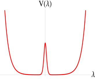
Figure 1: Effective potential $V(\lambda)$ for the scale factor.

We have explained that the phenomenological action (3.3) with $d=3$ is valid for a special class of solutions in superstring theory. In this paper, we investigate these solutions in which only the scale factors for 3 spacial dimensions are time dependent. The dynamics of this kind of cosmology has been studied before in several works [13, 17, 20] where solutions for the case $d=3$ have been found.

We should also be careful to point out that physical interpretation may depend on a chosen conformal frame. Unless we are able to fix the value of the dilaton $\phi$, we can not consistently conclude that the size of a dimension would remain small in the Einstein frame even if it becomes constant in the string frame. Nevertheless we may argue that the string frame is theoretically preferred to measure the size of the universe as T-duality holds in the string frame. Even with this limitation in mind, we will go ahead to study the cosmology in the string frame [5, 10, 14, 15, 23, 24, 25, 26].

3.1 Analytic solutions ($d=3$)

Now we present some analytic solutions that can be obtained by solving the equations of motion. First, we assume a simple equation of state $P_{\lambda}=wE$, with $w$ a constant and $P_{\varphi}=0$ (no dilaton potential). Using (3.8) and the equations of motion we get

$$\ddot{\varphi} = (1-\dot{\varphi}^{2})\left[1-(1-\dot{\varphi}^{2})^{1/2}\left((1-d\dot{\lambda}^{2})^{1/2}-\frac{H_{0}^{2}}{2^{d+1}}(\cosh 2\lambda)^{-d}\right)\right]$$ (3.12)

$$\ddot{\lambda} = (1-d\dot{\lambda}^{2})\left[\dot{\varphi}\dot{\lambda}+\gamma_{\lambda}^{-1}\left(\frac{H_{0}^{2}}{2^{d}}(\cosh 2\lambda)^{-d}\tanh 2\lambda+w(\gamma_{\varphi}-\gamma_{\lambda}-\frac{H_{0}^{2}}{2^{d+1}}(\cosh 2\lambda)^{-d})\right)\right]~{}$$ (3.13)

For the equation of state, we have three specific cases of interest: $w=0$, $w=1/d$ and $w=-1/d$, that correspond to pressureless matter, radiation dominated era and winding mode dominated era respectively. As the boundary condition for late time asymptotic behavior, we consider

$$\dot{\lambda}\rightarrow 0~{},~{}~{}\dot{\varphi}\rightarrow 0~{},~{}~{}|\lambda|\rightarrow\infty~{},~{}~{}\varphi\rightarrow-\infty~{}$$ (3.14)

In this limit, the equations of motion (3.12), (3.13) can be approximated as

$$\ddot{\lambda} = \dot{\varphi}\dot{\lambda}+H_{0}^{2}e^{-2d\lambda}+\frac{w}{2}(\dot{\varphi}^{2}-d\dot{\lambda}^{2}-H_{0}^{2}e^{-2d\lambda})$$ (3.15)

$$\ddot{\varphi} = \frac{1}{2}\dot{\varphi}^{2}+\frac{1}{2}d\dot{\lambda}^{2}+\frac{H_{0}^{2}}{2}e^{-2d\lambda}~{}$$ (3.16)

3.1.1 $H_{0}=0$, $w\neq 0$ case

We start with the standard string gas cosmology without 2-form field flux. For the case when $H_{0}=0$, we assume the following ansatz

$$\varphi = A\log t+B~{}$$ (3.17)

$$\lambda = C\log t+D~{}$$ (3.18)

After substituting them in (3.15) and (3.16), we find

$$\varphi = -\frac{2}{1+dw^{2}}\log t+B~{}$$ (3.19)

$$\lambda = \frac{2w}{1+dw^{2}}\log t+D~{}$$ (3.20)

This asymptotic solutions can be seen in figure 2 for $d=3$. We have plotted in the same figure the numerical solutions for the full equations of motion (3.12), (3.13) with $H_{o}=0$: momentum mode dominated universe (green line, $w=1/3$), dust dominated universe (blue line, $w=0$) and winding mode dominated universe (red line, $w=-1/3$). Of course the green and red lines are T dual to each other. The numerical solutions tend to the late time analytic solutions, which are plotted in figure 2 as gray dotted lines.

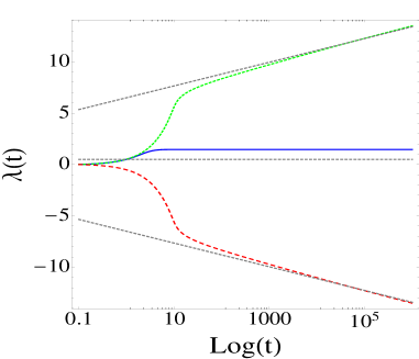
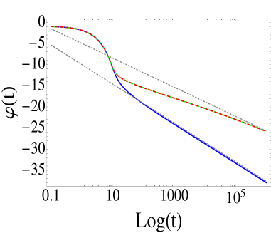
Figure 2: behavior of $\lambda$ and $\varphi$ with $H_{0}=0$ and $w=0$, $w=\frac{1}{3}$, $w=-\frac{1}{3}$. The gray dotted lines correspond to the late time analytic solutions.

From this solution we note that the scale factor goes to a constant value very quickly in the absence of any driving pressure. This behavior can be seen also in figures 2, 3, 4. The blue line in every picture represents the case when the effect of the pressure and the two-form field vanish, leading to the solution (3.19), (3.20) with $w=0$. Notice that this solution is valid for arbitrary $d$.

For completeness, we mention that there is an additional solution when $d=1$, $w=0$. In this special case, assuming $\dot{\varphi}=-\dot{\lambda}$, the equations of motion (3.15), (3.16) reduce to a differential equation in one variable $\ddot{\varphi}=\dot{\varphi}^{2}$, ($\ddot{\lambda}=-\dot{\lambda}^{2}$). Then we get the solution

$$\varphi = -\log(t+A)+B$$ (3.21)

$$\lambda = \log(t+A)+C$$ (3.22)

with $A$, $B$, $C$ constants. This solution is not physically relevant since we do not have the correct number of large space dimensions. Nevertheless, it is interesting to observe that a small coordinate can grow large even in the absence of any driving pressure.

3.1.2 $H_{0}\neq 0$, $w=0$ case

Now, we investigate a universe filled with dust ($w=0$) and an antisymmetric tensor potential ($H_{0}\neq 0$). Under this conditions, we substitute the ansatz (3.17) on equations (3.12), (3.13) to leading order as

$$\ddot{\varphi} = \frac{1}{2}\dot{\varphi}^{2}+\frac{1}{2}d\dot{\lambda}^{2}+\frac{H_{0}^{2}}{2}e^{-2d\lambda}~{}$$ (3.23)

$$\ddot{\lambda} = \dot{\varphi}\dot{\lambda}+H_{0}^{2}e^{-2d\lambda}~{}$$ (3.24)

Using ansatz (3.17), (3.18), we obtain

$$\varphi = \Big{(}-2+\frac{1}{d}\Big{)}\log t+B$$ (3.25)

$$\lambda = \frac{1}{d}\log t+\frac{1}{2d}\log\Big{(}\frac{H_{0}^{2}d^{2}}{d-1}\Big{)}$$ (3.26)

This analytic solution is plotted as gray colored straight lines in figure 3 for different values of $H_{0}$. Notice that $H_{0}$ fixes the initital value of $\lambda(t=1)$ in these solutions.

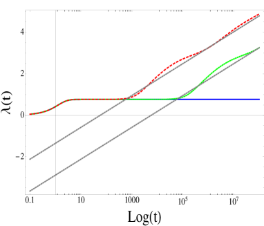
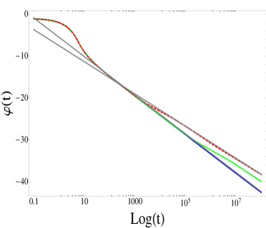
Figure 3: behavior of $\lambda$ and $\varphi$ when there is only the two-form field flux present ($W=0$, $K=0$, $H_{0}=0$, $H_{0}=0.001$, $H_{0}=0.0001$ ).

In this case we find that $H_{0}$ is able, by itself, to induce the growth of a large scale factor, as can be seen in figure 3. In this figure we can see how the two-form field flux induces decompactification for different values of $H_{0}$. Since the two-form field flux is along 3 spacial dimensions, in the absence of winding and momentum modes, this field alone is able to induce the growth of 3 large spacial dimensions. We also notice that the moment in which the scale factor is able to ”escape” the constant solution depends on the value of $H_{0}$. For larger values of it, the scale factor begins to increase earlier.

This kind of scenario, in which the two-form field flux happens to be the dominant term, can occur if the pressure coming from the winding and momentum modes becomes negligible ($P_{\lambda}\approx 0$). This happens in generic situations, for example, when the scale factor remains near the self-dual radius, the dilaton goes to weak coupling or when the winding and momentum modes have annihilated.

3.1.3 $H_{0}\neq 0$, $w\neq 0$ case

Finally we investigate the generic case when both the flux and the matter pressure are present. In order to find a solution when the antisymmetric tensor potential is present and the pressure fulfills the equation of state $P_{\lambda}=wE$, we use (3.12), (3.13) and the ansatz (3.14). Keeping only up to quadratic terms, we find

$$-\frac{A}{t^{2}} = \frac{A^{2}}{2t^{2}}+\frac{dC^{2}}{2t^{2}}+\frac{H_{0}^{2}}{2}e^{-2d(C\log t+D)}~{}$$ (3.27)

$$-\frac{C}{t^{2}} = \frac{AC}{t^{2}}+H_{0}^{2}e^{-2d(C\log t+D)}+\frac{w}{2}\left(\frac{A^{2}}{t^{2}}-\frac{dC^{2}}{t^{2}}-H_{0}^{2}e^{-2d(C\log t+D)}\right)~{}$$ (3.28)

By supposing that $C=\frac{1}{d}$, we can eliminate the $t^{-2}$ dependence on the equations. We obtain then

$$-A = \frac{A^{2}}{2}+\frac{1}{2d}+\frac{H_{0}^{2}}{2}e^{-2dD}$$ (3.29)

$$-\frac{1}{d} = \frac{A}{d}+H_{0}^{2}e^{-2dD}+\frac{w}{2}(A^{2}-\frac{1}{d}-H_{0}^{2}e^{-2dD})$$ (3.30)

Substituting $d=3$ explicitly and solving for $A$ and $D$, we find

$$A = \frac{5-3w}{3(w-1)}$$ (3.31)

$$H_{0}^{2}e^{-6D} = \frac{2-12w+6w^{2}}{9(w-1)^{2}}$$ (3.32)

In this way we find a solution

$$\varphi = \left(\frac{5-3w}{3(w-1)}\right)\log t+B$$ (3.33)

$$\lambda = \frac{1}{3}\log t-\frac{1}{6}\log\left(\frac{2-12w+6w^{2}}{9H_{o}^{2}(w-1)^{2}}\right)~{}$$ (3.34)

We observe, on equation (3.32) that $w$ is constrained by the inequality

$$w<1-\sqrt{\frac{2}{3}}\approx 0.1835~{}$$ (3.35)

It is not consistent with $w=1/3$ (radiation). This problem indicates that we cannot smoothly connect this solutions to those with $H_{0}=0$.

3.2 Perturbative solutions

3.2.1 $H_{0}\neq 0$, $w\neq 0$ case

Due to the difficulty we just encountered, we construct perturbative solutions with non-vanishing flux starting from those with no flux. Using the solutions we have obtained for the case when $H_{0}=0$, we treat the potential term due to $H_{0}\neq 0$ as a perturbation to the equations of motion. The small expansion parameter is

$$\delta\equiv H_{0}^{2}$$ (3.36)

We expand the solution in terms of the small parameter $\delta$

$$\varphi = \varphi_{0}+\delta\varphi_{1}+\delta^{2}\varphi_{2}+\cdots$$ (3.37)

$$\lambda = \lambda_{0}+\delta\lambda_{1}+\delta^{2}\lambda_{2}+\cdots$$ (3.38)

and substitute (3.37), (3.38) into the equations of motion. They describe perturbations around the solutions $\varphi_{0}$, $\lambda_{0}$ obtained in (3.19), (3.20).

From the power series expansion of the equation of motion (3.15), we get the differential equation for the first order terms in $\delta$

$$\ddot{\varphi}_{1} = \dot{\varphi_{0}}\dot{\varphi}_{1}+d\dot{\lambda_{0}}\dot{\lambda}_{1}+\frac{1}{2}e^{-2d\lambda_{0}}$$ (3.39)

$$\ddot{\lambda}_{1} = \dot{\varphi_{0}}\dot{\lambda}_{1}+\dot{\lambda_{0}}\dot{\varphi}_{1}+w(\dot{\varphi_{0}}\dot{\varphi}_{1}-\dot{\lambda_{0}}\dot{\lambda}_{1})+de^{-2d\lambda_{0}}(1-\frac{w}{2})~{}$$ (3.40)

After substituting $\varphi_{0}$, $\lambda_{0}$, $\dot{\varphi_{0}}$, $\dot{\lambda_{0}}$ into the equation, we obtain

$$\ddot{\varphi}_{1} = -\frac{2}{1+dw^{2}}t^{-1}\dot{\varphi}_{1}+\frac{2dw}{1+dw^{2}}t^{-1}\dot{\lambda}_{1}+\frac{1}{2}t^{-\frac{4dw}{1+dw^{2}}}e^{-2dD}~{}$$ (3.41)

$$\ddot{\lambda}_{1} = -\frac{2}{1+dw^{2}}t^{-1}\dot{\lambda}_{1}+\frac{2w}{1+dw^{2}}t^{-1}\dot{\varphi}_{1}+w(-\frac{2}{1+dw^{2}}t^{-1}\dot{\varphi}_{1}-\frac{2dw}{1+dw^{2}}t^{-1}\dot{\lambda}_{1})$$ (3.42)

$$\quad\quad\quad+dt^{-\frac{4dw}{1+dw^{2}}}e^{-2dD}(1-\frac{w}{2})~{}$$

For $\lambda_{1}$, we get a second order differential equation in this way

$$\ddot{\lambda}_{1}+2t^{-1}\dot{\lambda}_{1}-dt^{-\frac{4dw}{1+dw^{2}}}e^{-2dD}(1-\frac{w}{2})=0~{}$$ (3.43)

We can integrate this equation easily. Defining $x\equiv\dot{\lambda}_{1}$, $\dot{x}\equiv\ddot{\lambda}_{1}$ we get

$$\dot{x}+2t^{-1}x=t^{-\frac{4dw}{1+dw^{2}}}e^{-2dD}d(1-\frac{w}{2})~{}$$ (3.44)

This is a differential equation of the form $\dot{x}(t)+f(t)x(t)=g(t)$ and the solution is given by

$$x(t)=\frac{\int dt~{}g(t)e^{\int f(t)dt}+c}{e^{\int f(t)dt}}~{}$$ (3.45)

with a constant $c$.

After the integration, we find two different class of solutions:

• $\frac{4dw}{1+dw^{2}}\neq 3$ case.

  $$x=de^{-2dD}(1-\frac{w}{2})(3-\frac{4dw}{1+dw^{2}})^{-1}t^{-\frac{4dw}{1+dw^{2}}+1}+ct^{-2}$$ (3.46)

  $$\lambda_{1}=de^{-2dD}(1-\frac{w}{2})(3-\frac{4dw}{1+dw^{2}})^{-1}(2-\frac{4dw}{1+dw^{2}})^{-1}t^{-\frac{4dw}{1+dw^{2}}+2}-ct^{-1}+c_{0}$$ (3.47)

  Here, the leading perturbation contains two different time dependent terms. For the perturbation to be small, the exponent on the first term should fulfill the condition

  $$-\frac{4dw}{1+dw^{2}}+2<0~{}$$ (3.48)

  If it is the case, the influence of the two-form flux induced potential is negligible in comparison to the pressure of the string momentum modes. On the other hand, this condition is not satisfied for $w=0$ (pressureless dust) case where the perturbation grows as $t^{2}$. In such a situation the solution $\lambda_{0}$ is unstable and the universe is decompactified due to the presence of the two-form field flux.

• $\frac{4dw}{1+dw^{2}}=3$. This is the case for $d=3$ and a universe filled with radiation ($w=1/d$).

  $$x=s\frac{\log t}{t^{2}}+\frac{c}{t^{2}}$$ (3.49)

  $$\delta\lambda=-\frac{s+c}{t}-s\frac{\log t}{t}+c_{0}~{},\qquad s=-\frac{5}{2}H_{0}^{2}e^{-6D}~{}$$ (3.50)

  When $t\rightarrow\infty$, we find the leading perturbation as $\delta\lambda\sim\mathcal{O}(t^{-1})$ . Therefore the correction to the unperturbed solution is negligible at late time.

3.2.2 $H_{0}\neq 0$ case with both momentum and winding modes

As we observe in equation (3.10), the pressure coming from the winding modes and the momentum modes is multiplied by $e^{\varphi}$. If $|H_{0}|\ll 1$ and $|\varphi|\approx 1$, the scale factor experiences oscillations in the presence of winding and momentum modes. As $\varphi$ goes to weak coupling, oscillations stop and the pressure terms become small with respect to the $H_{0}^{2}$ potential term. Before this terms becomes significant, the solution is characterized as

$$\dot{\varphi}\approx 0,~{}\dot{\lambda}\approx 0,~{}\lambda\approx 0,e^{\varphi}\ll 1$$ (3.51)

We define a small parameter

$$\epsilon\equiv\frac{H_{0}^{2}}{2^{d}}$$ (3.52)

Under this approximation, keeping terms to the lowest nontrivial order, we get

$$\ddot{\varphi} = \frac{1}{2}(\dot{\varphi}^{2}+d\dot{\lambda}^{2}+\epsilon)$$ (3.53)

$$\ddot{\lambda} = \dot{\varphi}\dot{\lambda}+\epsilon\lambda$$ (3.54)

We expand the solution in terms of the small parameter $\epsilon$

$$\varphi = \varphi_{0}+\epsilon\varphi_{1}+\epsilon^{2}\varphi_{2}+\cdots$$ (3.55)

$$\lambda = \lambda_{0}+\epsilon\lambda_{1}+\epsilon^{2}\lambda_{2}+\cdots$$ (3.56)

After substituting (3.55), (3.56) into the equation of motion, we have differential equations at each order of the perturbation parameter

$$\ddot{\varphi}_{0} = \frac{1}{2}\dot{\varphi}_{0}^{2}+\frac{1}{2}d\dot{\lambda}_{0}^{2}$$ (3.57)

$$\ddot{\lambda}_{0} = \dot{\varphi}_{0}\dot{\lambda}_{0}$$ (3.58)

$$\ddot{\varphi}_{1} = \dot{\varphi}_{0}\dot{\varphi}_{1}+d\dot{\lambda}_{0}\dot{\lambda}_{1}+\frac{1}{2}$$ (3.59)

$$\ddot{\lambda}_{1} = \dot{\varphi}_{0}\dot{\lambda}_{1}+\dot{\lambda}_{0}\dot{\varphi}_{1}+\lambda_{0}$$ (3.60)

where the solutions for $\varphi_{0}$, $\lambda_{0}$ is given in equation (3.19), (3.20). Substituting them in (3.59), (3.60), we obtain

$$\ddot{\varphi}_{1} = -\frac{2}{t}\dot{\varphi}_{1}+\frac{1}{2}$$ (3.61)

$$\ddot{\lambda}_{1} = -\frac{2}{t}\dot{\lambda}_{1}+c_{0}$$ (3.62)

with $c_{0}$ a constant. These equations are linear differential equations in $\dot{\varphi}_{1}$ and $\dot{\lambda}_{1}$ respectively. They can be solved by multiplying them by the integrating factor $e^{(\int dt\frac{2}{t})}=e^{(2\log t)}=t^{2}$. The solutions are

$$\dot{\lambda}_{1}(t) = \frac{\lambda_{0}}{3}t+(const.)\quad\quad\lambda_{1}(t)=\frac{\lambda_{0}}{6}t^{2}+(const.)t^{-1}+const.$$ (3.63)

$$\dot{\varphi}_{1}(t) = \frac{1}{6}t+(const.)\quad\quad\varphi_{1}(t)=\frac{1}{12}t^{2}+(const.)t^{-1}+const.$$ (3.64)

We observe the following features: the solution $\varphi_{0},~{}\lambda_{0}$ becomes unstable if we perturbed it with nonvanishing $H_{0}$. To leading order the solution in this regime behaves like $\sim t^{2}$. This instability initiates an accelerated expansion of a universe away from the oscillating phase around the self-dual radius. However we also observe that the perturbation also affects the dilaton. As the perturbation becomes dominant, the dilaton begins to grow and goes to strong coupling. This indicates that a bounce on the dilaton has been produced. A result like this looks problematic, since a bounce on the dilaton leads to a violation on the positive energy condition as was noted in [16]. We may not be able to trust our solution there as it also takes the dilaton to strong coupling. This behavior can be observed directly in a numerical solution of the equations (figure 4). We begin with a string gas of equal number of winding modes and momentum modes. Before the dilaton goes to weak coupling, the scale factor oscillates around the self-dual radius. Once the dilaton reaches weak coupling region, the oscillations stop and the scale factor stabilizes. Then the potential induced by the two-form field flux becomes dominant and the solution begins to grow as predicted by the perturbed solution. In the next sub-section, we investigate the effects of the string interaction on these problems through the Boltzmann equations.

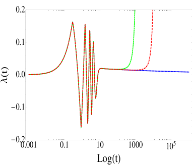
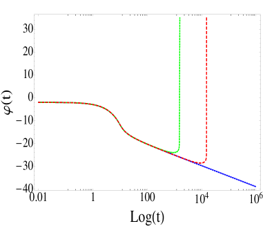
Figure 4: behavior of $\lambda$ in presence of $U(\lambda)$, winding and momentum modes ($W\neq 0,K\neq 0$, $H_{0}=0$, $H_{0}=0.01$, $H_{0}=0.001$ ).

3.3 Effects of string interactions

Up to this moment, we have considered situations in which the winding and momentum numbers are frozen at their initial values. When the string gas falls out of equilibrium in an expanding universe, winding strings in the gas can interact and begin to annihilate. In this section we incorporate, together with the two-form field flux induced potential, the Boltzmann equations that take account of the interaction among strings. These equations, derived by Polchinski [27], are shown below

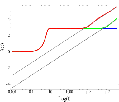
(a) $\lambda(t)$

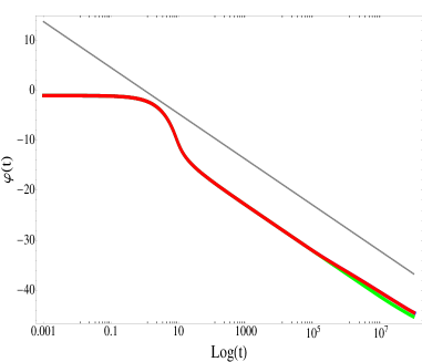
(b) $\varphi(t)$

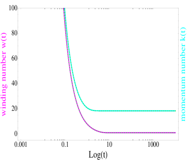
(c) $K(t),~{}W(t)$

Figure 5: (a), (b) behavior of $\lambda$ and $\varphi$ with initial condition $K=W$ for $H_{0}=0$, $H_{0}=0.001$ and $H_{0}=0.1$. The effect of the Boltzmann equations is included. (c) Evolution of the winding number and momentum number is plotted (the solutions overlap for the three cases considered).

.

$$\dot{W} = -\frac{e^{2\lambda+\varphi}}{\pi}(W^{2}-\langle W\rangle^{2})~{}$$ (3.65)

$$\dot{K} = -\frac{e^{-2\lambda+\varphi}}{\pi}(K^{2}-\langle K\rangle^{2})~{}$$ (3.66)

We combine these equations with (3.9), (3.10) and evolve the system numerically. The universe we consider is filled with gas of strings that begins at the self dual radius with equal initial winding and momentum numbers ($K=W$). The initial conditions are $\dot{\lambda}\approx 1$, $\dot{\varphi}\approx-1$ and the dilaton is going from strong coupling to weak coupling. The numerical results including the effects of the Boltzmann equations are presented in figure 5. We have plotted the behavior of the scale factor $\lambda(t)$, the dilaton $\varphi(t)$, the winding number $w(t)$ and the momentum number $k(t)$. In figure 5 we observe that, as $\lambda(t)$ grows, the winding modes begin to annihilate. Then, there is not enough pressure to make the universe contract and experience bounces. Instead, the contribution from the two-form field becomes dominant and the scale factor tends to the solution (3.25), (3.26) with vanishing pressure where the scale factor grows large due to the flux induced potential.

The behavior of the winding and the momentum number is as expected from the following characteristics of the Boltzmann equations (3.65), (3.66). As the dilaton goes to weak coupling, the interaction rate goes to zero and the values of the winding and momentum numbers become constant. When the scale factor grows large, winding modes annihilate more efficiently because their interaction rate goes as the exponential of the scale factor. On the contrary, the rate of annihilation of the momentum modes becomes smaller because the interaction rate between them decays exponentially with the scale factor. In fact this asymmetry between winding and momentum modes can be observed in figure 5(c).

The result obtained by taking account of the Boltzmann equations suggests an interesting scenario when homogeneous $H_{\mu\nu\lambda}$ is present. If the winding modes annihilate rapidly enough, the effect of 2-from field flux becomes important even at early times. The annihilation of the winding modes could take place even in a loitering phase. In that case the two-form field flux becomes dominant and the the expansion of three large spacial dimensions is realized. We emphasize that this mechanism is different from Brandenberger-Vafa mechanism as the presence of homogeneous 2-form field flux is crucial for three spacial dimensions to grow. Without it, the universe remains to be of microscopic size as the blue line in 5(a) indicates.

4 Effects of constant $B_{\mu\nu}$

So far, the effect of the two-form field has entered only as a modification to the usual dilaton gravity action, as in [14]. The string gas model, as it stands, couples the modified action of dilaton gravity with that of a gas of strings. In this approach the effect of the background field $B_{\mu\nu}$ over the string spectrum is usually neglected. The correction on the energy of the string goes as $\mathcal{O}(B)$, thus, this approximation is valid for weak fields. In dilaton-gravity, the contribution of $B_{\mu\nu}$ to the action enters via $U(\lambda)\sim|H|^{2}=|dB|^{2}$. In this case, even if $B$ remains small, $H$ is not necessary so as the space-time variation of $B_{\mu\nu}$ could be large.

In principle, if we know the two-form field in terms of the scale factors, we can determine $|H|^{2}$ as well as their effect on the string spectrum. We can then make use of the adiabatic approximation to study the time dependence of the compactification radii and get the equations of motion. In practice, a homogeneous solution for supergravity is given in terms of $H$. This presents a problem since we need $B_{\mu\nu}$, not $H$, in order to get the string spectrum.

With this prospect, we investigate the simplest case, that of a constant $B_{\mu\nu}$. In this case, the $H$ dependent term on the supergravity action vanishes as well as the contribution to the equations of motion. Nevertheless, since strings carry charge under the gauge field, the effect of $B$ field on closed strings wrapping the compact dimensions is non-trivial.

The Polyakov action in the presence of an antisymmetric field $B_{\mu\nu}$

$$S=-\frac{1}{\pi\alpha^{\prime}}\int d^{2}\sigma[\partial_{a}X^{\mu}\partial^{a}X_{\mu}-\epsilon^{ab}B_{\mu\nu}\partial_{\alpha}X^{\mu}\partial_{b}X^{\mu}]$$ (4.1)

yields the equations of motion

$$(\partial_{\tau}^{2}-\partial_{\sigma}^{2})X^{\mu}(\sigma,\tau)=-\frac{1}{2}{H^{\mu}}_{\lambda\nu}\epsilon^{ab}\partial_{a}X^{\lambda}\partial_{b}X^{\nu}$$ (4.2)

with $H_{\mu\nu\lambda}\equiv\partial_{\mu}B_{\nu\rho}+\partial_{\rho}B_{\mu\nu}+\partial_{\nu}B_{\rho\mu}~{}.$ Then, for a constant $B_{\mu\nu}$ we obtain the usual two dimensional wave equation

$$(\partial^{2}_{\tau}-\partial^{2}_{\sigma})X^{\mu}=0~{}$$ (4.3)

that allows us to give the solution in a Fourier-Laurent expansion

$$\dot{X}^{\mu}=\sqrt{\frac{\alpha^{\prime}}{2}}(\tilde{\alpha}_{0}+\alpha_{0})+\sqrt{\frac{\alpha^{\prime}}{2}}\sum_{n\neq 0}(\tilde{\alpha}_{n}e^{-in(\tau+\sigma)}+\alpha_{n}^{\mu}e^{-in(\tau-\sigma)})$$ (4.4)

$$X^{\prime\mu}=\sqrt{\frac{\alpha^{\prime}}{2}}(\tilde{\alpha}_{0}-\alpha_{0})+\sqrt{\frac{\alpha^{\prime}}{2}}\sum_{n\neq 0}(\tilde{\alpha}_{n}e^{-in(\tau+\sigma)}-\alpha_{n}^{\mu}e^{-in(\tau-\sigma)})~{}$$ (4.5)

As it turns out the zero-modes are the only ones that are affected by the $B_{\mu\nu}$ field. The components of the energy momentum tensor and their zero modes are given by

$$T^{01} = \frac{1}{2\pi\alpha^{\prime}}\partial^{0}X_{\mu}\partial^{1}X^{\mu}$$ (4.6)

$$= \frac{1}{2\pi\alpha^{\prime}}\bigg{[}\alpha^{\prime}p^{\mu}-{B^{\mu}}_{j}(wR)^{j}+\sqrt{\frac{\alpha^{\prime}}{2}}\sum_{n\neq 0}(\tilde{\alpha}_{n}^{\mu}e^{-in(\tau+\sigma)}+\alpha_{n}^{\mu}e^{-in(\tau-\sigma)})\bigg{]}$$

$$\times\bigg{[}(wR)_{\mu}+\sqrt{\frac{\alpha^{\prime}}{2}}\sum_{n\neq 0}(\tilde{\alpha}_{n\mu}e^{-in(\tau+\sigma)}-\alpha_{n\mu}e^{-in(\tau-\sigma)})\bigg{]}~{}$$

$$(T^{01})_{\text{zero~{}modes}}=n^{i}w_{i}+\frac{1}{2}\sum_{n=1}(\tilde{\alpha}_{n}\cdot\tilde{\alpha}_{-n}+\tilde{\alpha}_{-n}\cdot\tilde{\alpha}_{n}-\alpha_{-n}\cdot\alpha_{n}-\alpha_{n}\cdot\alpha_{-n})$$ (4.7)

$$T^{00} = \frac{1}{4\pi\alpha^{\prime}}(\dot{X}\cdot\dot{X}+X^{\prime}\cdot X^{\prime})$$ (4.8)

$$= \frac{1}{4\pi\alpha^{\prime}}\bigg{[}\bigg{(}\alpha^{\prime}p^{\mu}-{B^{\mu}}_{j}(wR)^{j}+\sqrt{\frac{\alpha^{\prime}}{2}}\sum_{n\neq 0}(\tilde{\alpha}_{n}e^{-in(\tau+\sigma)}+\alpha_{n}^{\mu}e^{-in(\tau-\sigma)})\bigg{)}^{2}$$

$$+\bigg{(}(wR)^{\mu}+\sqrt{\frac{\alpha^{\prime}}{2}}\sum_{n\neq 0}(\tilde{\alpha}_{n}^{\mu}e^{-in(\tau+\sigma)}-\alpha_{n}^{\mu}e^{-in(\tau-\sigma)})\bigg{)}^{2}\bigg{]}$$

$$(T^{00})_{\text{zero~{}modes}} = \frac{1}{\alpha^{\prime}}\bigg{[}-(\alpha^{\prime}p^{0}-{B^{0}}_{j}(wR)^{j})^{2}+(\alpha^{\prime}p^{i}-{B^{i}}_{j}(wR)^{j})^{2}+(wR)^{i}(wR_{i})$$ (4.9)

$$+\alpha^{\prime}\sum_{n=1}(\tilde{\alpha}_{n}\cdot\tilde{\alpha}_{-n}+\tilde{\alpha}_{-n}\cdot\tilde{\alpha}_{n}+\alpha_{n}\cdot_{-n}+\alpha_{-n}\cdot\alpha_{n})\bigg{]}$$

Imposing the physical constraint that the energy momentum tensor must vanish, we get the energy spectrum for the string

$$p^{0}=\frac{B^{0}_{j}w^{j}R}{\alpha^{\prime}}+\frac{1}{\alpha^{\prime}}\sqrt{\alpha^{\prime 2}\Big{(}\frac{n}{R}\Big{)}^{i}\Big{(}\frac{n}{R}\Big{)}_{i}+(wR)^{i}(wR)_{i}+{B^{i}}_{j}B_{ik}(wR)^{j}(wR)^{k}+\alpha^{\prime}B_{ik}n^{i}w^{k}+\alpha^{\prime}(\tilde{N}+N)}$$ (4.10)

and the level matching condition

$$\tilde{N}-N=n^{i}w_{i}~{}~{}$$ (4.11)

Since all the spacial coordinates are compactified with radius $R^{i}$, the momentum is quantized as $p^{i}=(n/R)^{i}$, where $i$ denotes the spacial index.

In order to be able to solve the equations of motion, we need to assume some initial winding and momentum distribution of the string gas. The constant $B_{\mu\nu}$ field could be either electric or magnetic type. We find that the effect of electric type field is very interesting as there is a critical value for which the string tension vanishes for winding modes.

4.1 Constant electric type field

Let’s consider the case of a homogeneous electric type field in 3-spacial dimensions, with $B\equiv B_{01}=B_{02}=B_{03}$. In order to demonstrate the most dramatic effect, we assume that strings are aligned in the direction of the electric type field. If this is the case, from (4.10), the energy for the winding modes in (2.21) is modified as

$$E_{W}=2d(1-\sqrt{3}B)We^{\lambda}~{}$$ (4.12)

with $W$ the winding number and $d=3$. From this equation, we see immediately that the effect of the field $B_{\mu\nu}$ is to reduce the energy of the winding strings. Also, it follows that $B$ is constrained to take values

$$0\leq B\leq\frac{1}{\sqrt{3}}~{}$$ (4.13)

In particular, when the inequality is saturated $B=1/\sqrt{3}$, the energy of the winding modes vanishes. As the pressure they exert also vanishes, the spacial dimensions are expected to expand freely because of the presence of the momentum modes.

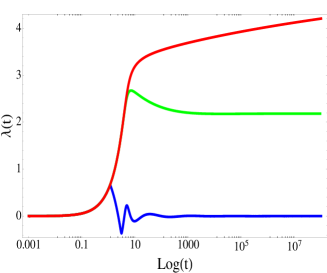
(a) Scale factor $\lambda$

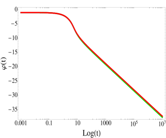
(b) Dilaton $\varphi$

.

Figure 6: behavior of the dilaton and scale factor for $B=0$, $B=0.5$, $B=1/\sqrt{3}$ (critical electric field) and $W=K$.

In figure 6 we have plotted the numerical solution for different values of $B$ without including the effect of the Boltzmann equations (3.65). For vanishing $B$ the momentum and winding modes make the scale factor oscillate around the self-dual radius. With small $B\neq 0$, the solutions oscillate around positive values of $\lambda$. As we get closer to the critical $B$, the solution bounces and then stabilizes. When we reach the critical value $B=1/\sqrt{3}$, the pressure from the winding modes becomes zero and $\lambda$ expands just like a universe filled with radiation (momentum modes).

5 Conclusions

In this work we have investigated some effects of the introduction of a two-form field into the model proposed in [16]. This model provides a bouncing and cycling cosmology and also the possibility of long loitering phases. It avoids singularities at finite times but fails to realize three large spacial dimensions from Brandenberger-Vafa mechanism. Having this in mind, we have included a two-form field into the action, since it may provide an alternative mechanism for the decompactification of 3 spacial dimensions. We have considered two cases: homogeneous flux $H_{\mu\nu\rho}$ and constant gauge field $B_{\mu\nu}$.

5.1 Homogeneous $H_{\mu\nu\rho}$

In order to make the model compatible with T-duality, as the string gas model requires, we have adopted a phenomenological modification on the potential induced by the two-form field entering the gravity action. The modified potential is non-singular at $\lambda=0$ and reduces to the correct one when the scale factor $|\lambda|$ is large. In addition, it provides a repulsive potential that can make the universe expand.

In the investigation of the behavior of the scale factor and the dilaton under the influence of the two-form field flux, we find two different cases:

• Matter dominance:
  At early times the scale factor can experience bounces as it is governed by the presence of winding and momentum modes. In section 3.2.2 we have observed that the effect of the two form field is not significant at this early stage of the universe. If we assume only the presence of the momentum modes, the late time solutions reduce to those already found in dilaton cosmology. If this solution is perturbed by the introduction of the two-form field flux potential, its influence vanishes as $t\rightarrow\infty$. On that account, this kind of solution is stable under the perturbation and the effect of $H_{\mu\nu\rho}$ is negligible as the universe expands.

• Two-form potential dominance:
  We have obtained the late time analytic solution for vanishing matter pressure and non-vanishing $H_{\mu\nu\rho}$. This solution corresponds to an expanding universe, where the initiation time of the expansion is set by the parameter $H_{0}$. This analytical solution matches the leading behavior of the numerical solution for the equations of motion.

  In generic situations the contribution of the matter pressure becomes negligible and the scale factor becomes constant. This occurs when the dilaton goes to weak coupling, the oscillations on the scale factor stop or the expansion of the universe comes to a halt. Such a possibility is enhanced if we consider the effect of interactions between strings. As momentum and winding modes can annihilate, it drives the pressure to vanish. In all of the above cases, the effect of the matter pressure vanishes and the scale factor becomes approximately constant. Introducing a $H_{\mu\nu\rho}$ flux, we find that the constant scale factor solution eventually becomes unstable and the scale factor begins to grow as

  $$\lambda\sim t^{2}~{}$$ (5.1)

  This kind of scenario occurs whenever the dilaton goes to weak coupling and the scale factor settles to a constant value. This behavior is remarkable, since it produces an accelerated expansion analogous to the inflationary universe. However we also need to address the issue that the perturbation to the dilaton also goes as $t^{2}$. Thus the dilaton may eventually bounce and go to strong coupling. The string interaction effect through the Boltzmann equation is observed to resolve these problems as in figure 5.

5.2 Constant $B_{\mu\nu}$

We have also investigated the case of a constant $B_{\mu\nu}$ in order to test how its presence affects the action of the string gas. For a constant field, the equations of motion for srings reduce to the usual one without $B_{\mu\nu}$. It is straightforward to include the effects of a constant B field by calculating the spectrum of the string. The inclusion of a constant $B_{\mu\nu}$ has some interesting consequences, one of these is that there is a critical value which makes the energy of the winding modes aligned with $B_{\mu\nu}$ field vanish.

We had expected the modification induced by $B_{\mu\nu}$ to be significant since its presence makes the energy and the pressure of the winding modes vanish at a critical value. In fact our numerical results indicate that the behavior of the scale factor could be significantly affected. The spacial directions expand like radiation dominated universe even with the presence of the both momentum and winding modes.

Appendix A Relation between string frame and Einstein frame

In this appendix, we summarize the relation between string frame and Einstein frame in our setup. The parameter $d$ in this appendix which counts the number of the spacial dimensions should be put $d=9$ in superstring. From the conformal transformation (2.7) and the corresponding metrics the relation between scale factors is

$$\alpha=-\frac{\phi}{d-1}+\lambda~{},\quad\beta=-\frac{\phi}{d-1}+\nu~{}$$ (A.1)

$$d\tilde{t}^{2}=e^{-\frac{2\phi}{d-1}}dt^{2}~{}$$ (A.2)

Also, the shifted dilaton is defined by

$$\varphi\equiv\phi-\sum_{i=1}^{d}\lambda_{i}~{}$$ (A.3)

Because of the presence of $H_{\mu\nu\lambda}$ for the superstring in ten dimensions, the spacial coordinates factorize as $T^{3}\times T^{6}$. Defining $\lambda_{i}\equiv\lambda$ for $i=\{1,2,3\}$ and $\lambda_{j}\equiv\nu$ for $j=\{4,\cdots,9\}$, we have $\varphi=\phi-3\lambda-6\nu$. Using the Einstein equations and the solution for the homogeneous two-form field, we obtain the equations of motion for the superstring case $(d=9)$

$$\dot{\varphi}^{2}-3\dot{\lambda}^{2}-6\dot{\nu}^{2} = e^{\varphi}E+U_{o}(\lambda)~{}$$ (A.4)

$$\ddot{\varphi}-3\dot{\lambda}^{2}-6\dot{\nu}^{2} = \frac{1}{2}e^{\varphi}E~{}$$ (A.5)

$$\ddot{\lambda}-\dot{\varphi}\dot{\lambda} = \frac{1}{2}P_{\lambda}+U_{o}(\lambda)~{}$$ (A.6)

$$\ddot{\nu}-\dot{\varphi}\dot{\nu} = \frac{1}{2}e^{\varphi}P_{\nu}~{}$$ (A.7)

with

$$U_{o}(\lambda)\equiv\frac{1}{12}H^{2}_{\alpha\beta\gamma}=\frac{1}{2}H_{o}^{2}e^{-6\lambda}~{}$$ (A.8)

Accordingly, the equations of motion in the Einstein frame are

$$6\alpha^{\prime 2}+36\alpha^{\prime}\beta^{\prime}+30\beta^{\prime 2} = \frac{\phi^{\prime 2}}{d-1}+e^{\frac{(d+1)\phi}{(d-1)}-3\alpha-6\beta}E+\frac{1}{2}H_{o}^{2}e^{{-6\alpha}-\frac{4\phi}{d-1}}~{}$$ (A.9)

$$\alpha^{\prime\prime}+\alpha^{\prime}(3\alpha^{\prime}+6\beta^{\prime}) = +\frac{3}{8}H_{o}^{2}e^{-6\alpha-\frac{4\phi}{d-1}}+\frac{1}{2\cdot 8}e^{\frac{(d+1)}{(d-1)}\phi-3\alpha-6\beta}(-5E+5P_{\lambda}-6P_{\nu})~{}$$ (A.10)

$$\beta^{\prime\prime}+\beta^{\prime}(3\alpha^{\prime}+6\beta^{\prime}) = -\frac{1}{8}H_{o}^{2}e^{-6\alpha-\frac{4\phi}{d-1}}+\frac{1}{2\cdot 8}e^{\frac{(d+1)}{(d-1)}\phi-3\alpha-6\beta}(3E-3P_{\lambda}+2P_{\nu})~{}$$ (A.11)

$$\phi^{\prime\prime}+\phi^{\prime}(3\alpha^{\prime}+6\beta^{\prime}) = H_{o}^{2}e^{-6\alpha-\frac{4\phi}{d-1}}+\frac{1}{2}e^{\frac{(d+1)}{(d-1)}\phi-3\alpha-6\beta}(3P_{\lambda}+6P_{\nu})~{}$$ (A.12)

In the string frame, the equation of motion for $\lambda$ contains the dilaton and its time derivative but it does not contain $\nu$ terms. In the same way the equation of motion for $\nu$ is independent of $\lambda$ or its time derivatives. Then, the equations of motion for the scale factors $\nu$ and $\lambda$ decouple and we can proceed to solve them numerically. In comparison, in the Einstein frame, the presence of $\tilde{H}_{\mu\nu\lambda}$ makes the scale factors couple to each other. In spite of this unfavourable characteristic, the equations of motion in the Einstein frame are also useful, both when trying to solve the equations of motion and also for clarifying the interpretation of the solutions.

In the Einstein frame the field $\tilde{H}_{\mu\nu\lambda}$ is included in the equation of motion for both $\alpha$ and $\beta$. By looking at the sign of the $H_{o}$ term in (A.10) and (A.11) we can see that the two-form field induces an anisotropic expansion on the scale factors, with $\phi$ and $\alpha$ being driven towards positive values while $\beta$ goes towards negative values. Also, while in the string frame it is possible to find solutions to the equations of motion in which $\nu$ becomes constant, this does not imply that the physical scale factor is fixed because it remains to stabilize the value of the dilaton. This can be seen directly from the relations of the Einstein frame to the string frame, where, in the case of $\nu=constant$ we have

$$\beta=-\frac{\phi}{d-1}+{\text{c}onst}.$$ (A.13)

That is, unless both the dilaton $\phi$ and $\nu$ are constant in the string frame, there is no solution with $\beta=constant$ in the Einstein frame.

References

- [1] R. H. Brandenberger and C. Vafa, “Superstrings in the Early Universe,” Nucl. Phys. B 316, 391 (1989).
- [2] R. H. Brandenberger, “String Gas Cosmology,” arXiv:0808.0746 [hep-th].
- [3] A. A. Tseytlin and C. Vafa, “Elements Of String Cosmology,” Nucl. Phys. B 372, 443 (1992) [arXiv:hep-th/9109048].
- [4] A. A. Tseytlin, “Dilaton, winding modes and cosmological solutions,” Class. Quant. Grav. 9, 979 (1992) [arXiv:hep-th/9112004].
- [5] T. Battefeld and S. Watson, “String gas cosmology,” Rev. Mod. Phys. 78, 435 (2006) [arXiv:hep-th/0510022].
- [6] M. Sakellariadou, “Numerical Experiments in String Cosmology,” Nucl. Phys. B 468, 319 (1996) [arXiv:hep-th/9511075].
- [7] G. B. Cleaver and P. J. Rosenthal, “String cosmology and the dimension of space-time,” Nucl. Phys. B 457, 621 (1995) [arXiv:hep-th/9402088].
- [8] B. A. Bassett, M. Borunda, M. Serone and S. Tsujikawa, “Aspects of string-gas cosmology at finite temperature,” Phys. Rev. D 67, 123506 (2003) [arXiv:hep-th/0301180].
- [9] D. A. Easson, “Brane gases on K3 and Calabi-Yau manifolds,” Int. J. Mod. Phys. A 18, 4295 (2003) [arXiv:hep-th/0110225].
- [10] B. Greene, D. Kabat and S. Marnerides, “Dynamical Decompactification and Three Large Dimensions,” arXiv:0908.0955 [hep-th].
- [11] Hajime Aoki, Satoshi Iso, Hikaru Kawai, Yoshihisa Kitazawa, Tsukasa Tada, “Space-time structures from IIB matrix model,” Prog. Theor. Phys. 99, 713 (1998).
- [12] Takaaki Imai, Yoshihisa Kitazawa, Yastoshi Takayama, Dan Tomino, “Effective actions of matrix models on homogeneous spaces,” Nucl. Phys. B679, 143 (2004).
- [13] E. J. Copeland, A. Lahiri and D. Wands, “String cosmology with a time dependent antisymmetric tensor potential,” Phys. Rev. D 51, 1569 (1995) [arXiv:hep-th/9410136].
- [14] A. Campos, “Late cosmology of brane gases with a two-form field,” Phys. Lett. B 586, 133 (2004) [arXiv:hep-th/0311144].
- [15] A. Campos, “Asymptotic cosmological solutions for string / brane gases with solitonic fluxes,” Phys. Rev. D 71, 083510 (2005) [arXiv:hep-th/0501092].
- [16] B. Greene, D. Kabat and S. Marnerides, “Bouncing and cyclic string gas cosmologies,” arXiv:0809.1704 [hep-th].
- [17] D. S. Goldwirth and M. J. Perry, “String Dominated Cosmology,” Phys. Rev. D 49, 5019 (1994) [arXiv:hep-th/9308023].
- [18] J. Ambjorn, Y. M. Makeenko, G. W. Semenoff and R. J. Szabo, “String theory in electromagnetic fields,” JHEP 0302, 026 (2003) [arXiv:hep-th/0012092].
- [19] G. Grignani, M. Orselli and G. W. Semenoff, “The target space dependence of the Hagedorn temperature,” JHEP 0111, 058 (2001) [arXiv:hep-th/0110152].
- [20] J. E. Lidsey, D. Wands and E. J. Copeland, Phys. Rept. 337, 343 (2000) [arXiv:hep-th/9909061].
- [21] Charles Misner and Kip Thorne and John Wheeler, “Gravitation”, (1973)
- [22] P. G. O. Freund and M. A. Rubin, “Dynamics of dimensional reduction”, Phys. Lett. B Volume 97, Issue 2, 1 December 1980, Pages 233-235.
- [23] S. Alexander, R. H. Brandenberger and D. Easson, “Brane gases in the early universe,” Phys. Rev. D 62, 103509 (2000) [arXiv:hep-th/0005212].
- [24] R. Easther, B. R. Greene and M. G. Jackson, “Cosmological string gas on orbifolds,” Phys. Rev. D 66, 023502 (2002) [arXiv:hep-th/0204099].
- [25] R. Easther, B. R. Greene, M. G. Jackson and D. N. Kabat, “Brane gases in the early universe: Thermodynamics and cosmology,” JCAP 0401, 006 (2004) [arXiv:hep-th/0307233].
- [26] R. Easther, B. R. Greene, M. G. Jackson and D. N. Kabat, “String windings in the early universe,” JCAP 0502, 009 (2005) [arXiv:hep-th/0409121].
- [27] J. Polchinski, “Collision Of Macroscopic Fundamental Strings,” Phys. Lett. B 209, 252 (1988).
- [28] S. Watson and R. H. Brandenberger, “Isotropization in brane gas cosmology,” Phys. Rev. D 67, 043510 (2003) [arXiv:hep-th/0207168].