Thermal conductivity in dynamics of first-order phase transitions

Abstract

Effects of thermal conductivity on the dynamics of first-order phase transitions are studied. Important consequences of a difference of the isothermal and adiabatic spinodal regions are discussed. We demonstrate that in hydrodynamical calculations at non-zero thermal conductivity, $\kappa\neq 0$, onset of the spinodal instability occurs, when the system trajectory crosses the isothermal spinodal line. Only for $\kappa=0$ it occurs at a cross of the adiabatic spinodal line. Therefore ideal hydrodynamics is not suited for an appropriate description of first order phase transitions.

and

1 Introduction

There are numerous phenomena, where first-order phase transitions occur between phases of different densities. In nuclear physics various first-order phase transitions may take place in the Early Universe [1], in heavy ion collisions [2, 3] and in neutron stars (e.g., pion, kaon condensation and deconfinment or chiral phase transition [4, 5]). At low collision energies the nuclear gas-liquid (nGL) first-order phase transition is possible [2, 6, 7, 8, 9]. The experimental status of the latter is discussed in Refs. [10, 11, 12]. At high collision energies the hadron – quark gluon plasma (hQGP) first-order phase transition may occur (see e.g. Ref. [3]). Within the hydrodynamical approach dynamical aspects of the nGL and hQGP transitions have been recently studied in Refs. [13, 14, 15]. An important role of effects of non-ideal hydrodynamics has been emphasized in Ref. [13, 14]. However in these works density fluctuations were carefully analyzed, whereas thermal transport effects were only roughly estimated.

Dynamical trajectories of the system in heavy-ion collisions can be approximately determined by constant initial values of the entropy per baryon (i.e. entropy density per net baryon density). This conclusion follows from the analysis of heavy ion collisions at energies less than several GeV$/A$ performed in an expanding fireball model (e.g., see Ref. [16]), from ideal hydrodynamical calculations in a broad energy range (see e.g. Refs. [17, 18]) and also from transport calculations (e.g., see Ref. [19]).

It is well known, see Refs. [15, 20, 21], that, at least in the mean field approximation, the isothermal spinodal (ITS) line and adiabatic spinodal (AS) line are different. From the exact thermodynamic relation one obtains

$$u_{\tilde{s}}^{2}=u_{T}^{2}+\frac{T}{nmc_{V}}\left[\left(\frac{\partial P}{\partial T}\right)_{n}\right]^{2}.$$ (1)

Here $T$ is the temperature, $P$ is the pressure, $n$ is the density of the conserving charge (here the baryon density), $m$ is the baryon mass, $\tilde{s}\equiv s/n$ is the entropy per baryon, $c_{V}$ is the specific heat density at the fixed volume $V$, $u_{\tilde{s}}^{2}=m^{-1}(\partial P/\partial n)_{\tilde{s}}$ and $u_{T}^{2}=m^{-1}(\partial P/\partial n)_{T}$. The value $u_{\tilde{s}}$ has the meaning of the adiabatic sound velocity (at $\tilde{s}=$const). Namely, this quantity characterizes propagation of sound waves in ideal hydrodynamics. As we show below, in non-ideal hydrodynamics at a finite value of the thermal conductivity, $\kappa$, the propagation of sound waves is defined by the interplay between $u_{T}$ (at $T=$const) and $u_{\tilde{s}}$. Conditions $u_{T}=0$ and $u_{\tilde{s}}=0$ define $T(n)$-curves: the ITS line (at fixed temperature $T$) and AS line (at fixed $\tilde{s}$), respectively. The maximum temperature points on these lines are the critical temperature $T_{cr}$ in case of $T$=const and the adiabatic maximum temperature $T_{P,max}$ in case of $\tilde{s}=$const. In the mean field approximation, the specific heat density $c_{V}$ has finite non-negative values. Thus one has $u_{T}^{2}\leq 0$ on the AS line, where $u_{\tilde{s}}=0$.

Calculations performed in mean field models show that $T_{cr}\geq T_{P,max}$. In Refs. [7, 9] and numerous subsequent works, crossing of the AS line by effective trajectories $\tilde{s}$=const was considered as the starting point for the multifragmentation following an adiabatic expansion of the system. In contrast, in Ref. [8] and later Refs. [21, 22, 23] it was assumed that the multifragmentation may appear already at higher temperatures, when the ITS curve is crossed by the $\tilde{s}$=const lines. The argumentation of the former group of works can be traced back to the fact that in ideal hydrodynamics instabilities indeed arise at the AS boundary (see extensive discussions in Ref. [15]). Isothermal instabilities at first order phase transitions were studied in details in Refs. [13, 14].

In mean field theories, difference between values of $T_{cr}$ and $T_{P,max}$ is usually rather large. For example, within the NJL model one obtains $T_{P,max}\sim T_{cr}/2\simeq 45$ MeV (see Ref. [21]) for the chiral restoration transition. In the model used in Ref. [15] $T_{P,max}=3T_{cr}/5\simeq 100$ MeV for hQGP phase transition. Note that simultaneously with the low value $T_{P,max}\sim(50\div 100)$ MeV a sufficiently high value of $n_{P,max}$ should be reached. This looks unlikely to be achieved in heavy-ion collisions. Hence, if instability occurs for $T<T_{P,max}$, one could face difficulties in exploring the hQGP spinodal instabilities in actual experiments with heavy ions.

It was argued in Ref. [21] that above mentioned difference of $T_{cr}$ and $T_{P,max}$ is probably an artifact of the mean field approximation and both values of the critical temperature should coincide provided thermal fluctuation effects are included. Indeed, it is known (e.g., see  Ref. [24]), that inclusion of fluctuations may result in a weak divergence of the specific heat. For example, for the three-dimensional Ising universality class $c_{V}\sim[(T-T_{c})/T_{c}]^{-\alpha}$, where $\alpha\simeq 0.12$. It can be concluded from Eq. (1), that for divergent $c_{V}$ both temperatures $T_{cr}^{\rm fl}$ and $T_{P,max}^{\rm fl}$ should coincide. Although this observation is fully true, it seems legitimate to rise some questions.

• First, thermal fluctuation effects are strong enough only in a critical region, where the mean field theory breaks down and system properties are governed by non-trivial critical exponents. For many systems the critical region is a rather narrow region near the critical point, while contrary examples are known as well [24]. Although it is not known a priori how large is the hQGP critical region, there is an indication in favor of the hQGP critical region being small [25]. Only if the system trajectory passes trough the critical region, one can hope that fluctuation effects appearing during evolution of the system may lead to $T_{cr}^{\rm fl}\simeq T_{P,max}^{\rm fl}$.

• Second, even if the system trajectory passes through the critical region and $T_{cr}^{\rm fl}$ coincide with $T_{P,max}^{\rm fl}$, the ITS and the AS lines may not collapse into one line even within the critical region because the fluctuation contribution to the specific heat diverges only at the critical point and then sharply decreases. Thus we should understand crossing of which of two lines (the ITS or AS line) results in the spinodal instability.

• Third, the divergence of $c_{V}$ at the critical point is due to long-scale fluctuations, which need a long time to develop. Therefore the time, which the system spends in a vicinity of the critical point in the course of the heavy ion collision, might be insufficient for the developing of such fluctuations, see discussions in Refs. [13, 14, 26, 27].

Moreover, if the initial collision energy is such that the system trajectory passes outside the critical region, i.e. entirely in the mean field regime, the thermal fluctuation effects do not contribute at all. Then the question arises how one can treat the problem purely within the mean field approximation. This is actually an important question, since most of equations of state used in the description of heavy ion collisions disregard the fluctuation effects.

In Refs. [13, 14] we focused on the study of dynamical effects of the viscosity and the surface tension. The aim of the given paper is to consider the influence of thermal conductivity effects on the dynamics of first-order phase transitions and to answer above risen questions. Below we find out that in non-ideal hydrodynamics (with non-zero thermal conductivity, $\kappa\neq 0$) instabilities show up at the crossing of the ITS line and only for $\kappa=0$, e.g. in ideal hydrodynamics, they appear at the AS line.

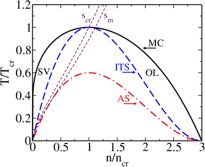
Figure 1: Phase diagram of the Van der Waals equation of state, $T(n)$-plane. Bold solid, dashed and dash-dotted curves demonstrate boundaries of the Maxwell construction, the spinodal region at $T=$const and $\tilde{s}=$const, respectively. The short dash lines show adiabatic trajectories of the system evolution, see explanation in the text.

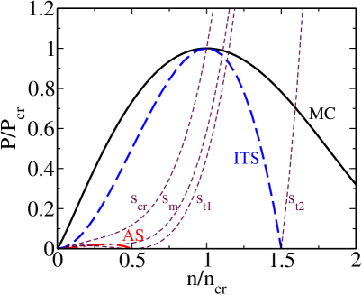
Figure 2: Phase diagram for the Van der Waals equation of state in $P(n)$ plane, see explanation in the text.

2 General setup

To simplify further considerations we describe the dynamics of a first-order phase transition by means of the standard system of equations of non-ideal non-relativistic hydrodynamics: the Navier-Stokes equation, the continuity equation, and the general equation for the heat transport:

$$mn\left[\partial_{t}{u}_{i}+(\mathbf{u}\nabla){u}_{i}\right]=-\nabla_{i}P$$ (2)

$$+\nabla_{k}\left[\eta\left(\nabla_{k}u_{i}+\nabla_{i}u_{k}-\frac{2}{d}\delta_{ik}\mbox{div}\mathbf{u}\right)+\zeta\delta_{ik}\mbox{div}\mathbf{u}\right],$$

$$\partial_{t}n+\mbox{div}(n\mathbf{u})=0,$$ (3)

$$T\left[\frac{\partial s}{\partial t}+\mbox{div}(s\mathbf{u})\right]=\mbox{div}(\kappa\nabla T)$$ (4)

$$+\eta\left(\nabla_{k}u_{i}+\nabla_{i}u_{k}-\frac{2}{d}\delta_{ik}\mbox{div}\mathbf{u}\right)^{2}+\zeta(\mbox{div}\mathbf{u})^{2}.$$

Here $\eta$ and $\zeta$ are the shear and bulk viscosities; $\mathbf{u}$ is the velocity of the fluid element; $s$ is the entropy density; $\kappa$ is the thermal conductivity; $d$ is the dimensionality of space. The short-scale fluctuations can be taken into account by adding noise terms on the right sides of Eqs. (2-4). In what follows we neglect these contributions.

Before we proceed further we aware the reader, that Eqs. (2-4) are derived in the first gradient order approximation, see Ref. [28]. In the kinetic regime the typical inverse relaxation time of the system $\tau_{\rm rel}^{-1}$ and the typical inverse spatial scale $k_{\rm kin}$ characterizing the collective processes fulfil the inequalities $\tau_{\rm rel}^{-1}\ll\epsilon_{\rm ch}$ and $k_{\rm kin}\ll p_{\rm ch}$, see [29], where $\epsilon_{\rm ch}$ and $p_{\rm ch}$ characterize microscopic processes. For quasi-equilibrium nucleon system with $T\stackrel{{\scriptstyle\scriptstyle>}}{{\phantom{}{}_{\sim}}}\epsilon_{\rm F}$ ($\epsilon_{\rm F}$ is the nucleon Fermi energy) one has $\epsilon_{\rm ch}\sim T$ and $p_{\rm ch}\sim p_{T}=\sqrt{2mT}$. The hydrodynamic regime is reached if the typical time scale and the typical length scale characterizing the collective motion are larger than the corresponding kinetic values, $\tau_{\rm hydro}\gg\tau_{\rm rel}$ and $l_{\rm hydro}\gg 1/k_{\rm kin}$. In what follows we assume that these inequalities are fulfilled.

An approximate validity of the adiabatic expansion (i.e. conservation of specific entropy density, $\tilde{s}$, along the fluid flow) in heavy ion collisions [19] means that (i) $\kappa$ is rather small, or the system is spatially homogeneous and (ii) $\eta$ and $\zeta$ are small, or the velocity of the expansion of the system is very low (with the guaranty for absence of shock waves). Note that in the general case solutions of Ref. [13], which we will exploit below, are obtained at a non-zero viscosity therefore we will not additionally assume smallness of the viscosity coefficients, rather we exploit smallness of the velocity $u$.

The best known example to illustrate principal features of a first order phase transition in the mean field approximation is the Van der Waals fluid. Expressions for thermodynamical quantities in this particular case are presented in Appendix A. Trajectories for the expansion of the uniform system, obtained at the assumption $\tilde{s}\simeq$ const, are shown in Fig. 1 on the plot $T/T_{cr}=f(n/n_{cr})$. The upper convex curve (MC, bold solid line) is the boundary of the Maxwell construction, the next bold dashed line (ITS) shows the boundary of the ITS region and the lower bold dash-dotted curve (AS), the boundary of the AS region. The short dashed lines crossing the regions under these three curves are calculated at two values of the entropy per baryon: $\tilde{s}_{cr}$ and $\tilde{s}_{m}$. Different scenarios of the dynamics for first-order phase transitions in expanding system at $\tilde{s}\simeq$ const have been considered previously in Ref. [8]. The super-cooled vapor (SV) and the overheated liquid (OL) regions are between the MC (bold solid curve) and the ITS (bold dash) curves, on the left and on the right respectively. For $\tilde{s}_{cr}>\tilde{s}>\tilde{s}_{\rm MC2}$, where $\tilde{s}_{cr}$ corresponds to the critical point and the line with $\tilde{s}_{\rm MC2}$ passes through the point $n/n_{cr}=3$ at $T=0$, the system traverses the OL state (region OL in Fig. 1) and then the ITS region (below ITS line) and the AS region (below AS line). For $\tilde{s}>\tilde{s}_{cr}$ the system trajectory passes through the SV state (the region SV in Fig. 1) and then the ITS region.

In Fig. 2 we show the same regions as in Fig.1, but in the plane $P/P_{cr}-n/n_{cr}$ for $P>0$. The line $\tilde{s}_{m}$ corresponds to the maximum pressure at the AS curve. The critical point is determined by $(dP/dn)_{T}=0$, $(d^{2}P/dn^{2})_{T}=0$. With the help of Eq. (37) of Appendix A from these conditions we find $n_{cr}=1/(3b)$, $T_{cr}=8a/(27b)$. The maximal pressure point at AS line is defined by $(dP/dn)_{\tilde{s}}=0$, $(d^{2}P/dn^{2})_{\tilde{s}}=0$. Thus using Eq. (40) we obtain: $n_{P,max}=1/(9b)=n_{cr}/3$, $T_{P,max}=128a/(1215b)=16T_{cr}/45$, see Fig. 2. The maximal temperature point on the AS curve corresponds to $T_{max}=3/5T_{cr}$, $n_{max}=n_{cr}$, see Fig. 1. Another relevant point on each line $\tilde{s}={\rm const}$ is the turning point, where $E(n,\tilde{s}={\rm const})$ has a minimum as a function of the density, $n$. In this point the pressure $P(n,\tilde{s}={\rm const})$ equals zero and the fireball expansion is slowing down. The lines labeled $\tilde{s}_{t1}$ and $\tilde{s}_{t2}$ cross respectively the AS and ITS lines at $P=0$. Note, that with realistic equation of state, $P=0$ might be reached at the nGL first-order phase transition, see Ref. [20], but not at the hQGP transition.

We stress that we use the Van der Waals equation of state only for the illustrative purpose. Our main conclusions do not depend on the used equation of state provided there is a first order phase transition.

We may expand all quantities near an arbitrary reference point $(n_{\rm r},T_{\rm r})$, or $(n_{\rm r},\tilde{s}_{\rm r})$. Analytical solutions can be found, provided the system is in the vicinity of the critical point $(n_{cr},T_{cr})$, or near the maximum point $(n_{P,max},\tilde{s}_{P,max})$. Therefore considering the problem in $(n,T)$ variables it is convenient to take $(n_{cr},T_{cr})$ as the reference point and considering the problem in $(n,\tilde{s})$ variables, to take $(n_{P,max},\tilde{s}_{P,max})$ as the reference point. The following remark is in order. As we have mentioned, in this paper we exploit the mean field approximation. Thus using $(n_{cr},T_{cr})$ as the reference point we actually assume that the fluctuation region ($n_{cr}\mp\delta n^{\rm fl}$, $T_{cr}\mp\delta T^{\rm fl}$) is very narrow and we are able to chose the reference point outside this region (but nevertheless very close to the critical point). Also, mentioned problem is avoided provided one considers the system at the time scale, being shorter than that necessary for a development of long-scale critical fluctuations.

We construct the generating functional in ($\delta n=n-n_{cr}$, $\delta T=T-T_{cr}$) or in ($\delta n=n-n_{P,max}$, $\delta\tilde{s}=\tilde{s}-\tilde{s}_{P,max}$) variables, the Landau free energy, such that $\delta(\delta F_{L})/\delta(\delta n)=P-P_{f}+P_{\rm MC}$:

$$\delta F_{L}=\int\frac{d^{3}x}{n_{cr}}\left\{\frac{cm[\nabla(\delta n)]^{2}}{2}+\frac{\lambda m^{3}(\delta n)^{4}}{4}-\frac{\lambda v^{2}m(\delta n)^{2}}{2}-\epsilon\delta n\right\},$$ (5)

where $\epsilon=P_{f}-P_{\rm MC}$ is expressed through the pressure on the Maxwell construction. The maximum of the quantity $\epsilon$ is ${\epsilon}^{m}=4\lambda v^{3}/(3\sqrt{3})$, therefore we may count ${\epsilon}$ from this value supposing further that ${\epsilon}=\pm\gamma_{\epsilon}{\epsilon}^{m}$ with $0<\gamma_{\epsilon}<1$. The first term in Eq. (5) is due to the surface tension. It produces a surface pressure $P_{surf}$ (see Eq. (10) below).

In case of the Van der Waals form of the equation of state, see Appendix A, expanding the pressure of the uniform matter in $\delta n=n-n_{cr}$, $\delta T=T-T_{cr}$, for $|\delta n|/n_{cr}\ll 1$, $|\delta{T}|/T_{cr}\ll 1$, i.e. in the vicinity of the critical point $(n_{cr},T_{cr})$, we obtain

$$\delta P[n,T]=f_{0}\left[\frac{9\delta{{T}}\delta n}{4}+\frac{9T_{cr}(\delta n)^{3}}{16n_{cr}^{2}}+\frac{3}{2}n_{cr}\delta T+...\right].$$ (6)

The last explicitly presented term in Eq. (6) is unimportant if $T(\vec{r})\simeq$ const, since the addition of any constant does not change equation of motion (2).

Comparing Eq. (6) with the value, which follows from Eq. (5), we find relations between coefficients:

$$v^{2}(T)=-4\delta{{T}}n_{cr}^{2}m^{2}/T_{cr},$$

$$\lambda_{cr}=\frac{9f_{0}}{16}\frac{T_{cr}}{n_{cr}^{2}m^{3}}.$$ (7)

Expanding the pressure with respect to $\delta n=n-n_{P,max}$, $\delta\tilde{s}=\tilde{s}-\tilde{s}_{P,max}$ in the vicinity of the maximum of $P(n)$ at fixed ${\tilde{s}}$ we obtain

$$\delta P[n,\tilde{s}]=\frac{15}{512}T_{P,max}\left[\delta\tilde{s}\delta n+\frac{f_{0}(\delta n)^{3}}{2n_{P,max}^{2}}+\frac{114}{15}n_{P,max}\delta\tilde{s}+...\right].$$ (8)

Comparing this expression with the value, which follows from Eq. (5), we find relations

$$v^{2}(\tilde{s})=-2\delta{\tilde{s}}n_{P,max}^{2}m^{2}/f_{0},$$

$$\lambda_{P,max}=\frac{15f_{0}}{1024}\frac{T_{P,max}}{n_{P,max}^{2}m^{3}}.$$ (9)

Further, following Refs. [13, 14], we use smallness of the velocity $\mathbf{u}(t,\mathbf{r})$ of the growth/damping of the density and temperature fluctuations. We linearize all terms in hydrodynamical equations in the velocity $\mathbf{u}\,$, the entropy density $\delta s=s-s_{\rm r}$ and the temperature $\delta T=T-T_{\rm r}$ variables. Here index “r” stays for an arbitrary reference point.

Excluding a dependence on the velocity, $\mathbf{u}$, from Eqs. (2), (2) we obtain [13, 14, 30]

$$m\partial^{2}_{t}\delta n=\Delta\left[P+P_{surf}-P_{f}+n_{\rm r}^{-1}\left(\tilde{d}\eta_{\rm r}+\zeta_{\rm r}\right)\partial_{t}\delta n\right],$$ (10)

where $P_{surf}$ is the surface pressure; $\tilde{d}=2(d-1)/d$, $\tilde{d}=4/3$ for spherical geometry, $\delta n=n-n_{\rm r}$. We count $P$ from its value in the final equilibrium state (reached at $t\rightarrow\infty$). Namely this difference, $P-P_{f}$, has the meaning of the thermodynamical force driving the system to the final equilibrium state.

Eq. (10) should be supplemented by the equation for the heat transport (4), which after linearization owing to Eq. (2) simplifies as

$$T_{\rm r}\left[\partial_{t}\delta s-s_{\rm r}(n_{\rm r})^{-1}\partial_{t}\delta n\right]=\kappa_{\rm r}\Delta\delta T.$$ (11)

The variation of the temperature is related to the variation of the entropy density $s[n,T]$ by

$$\delta T\simeq T_{\rm r}(c_{V,\rm r})^{-1}\left(\delta s-({\partial s}/{\partial n})_{T,\rm r}\delta n\right),$$ (12)

where, as in Eq. (1), $c_{V,\rm r}$ is the specific heat density.

3 Instabilities in spinodal region

3.1 Effect of finite thermal conductivity

Since in this section the “r”-reference point can be taken arbitrary, we suppress index “r”. To find solutions of hydrodynamical equations we present, cf. [13, 14, 15],

$$\delta n=\delta n_{0}\mbox{exp}[\gamma t+i\mathbf{p}\mathbf{r}],$$

$$\delta s=\delta s_{0}\mbox{exp}[\gamma t+i\mathbf{p}\mathbf{r}],$$ (13)

$$T=T_{>}+\delta T_{0}\mbox{exp}[\gamma t+i\mathbf{p}\mathbf{r}].$$

where $T_{>}$ is the temperature of the uniform matter.

For finite thermal conductivity, $\kappa\neq 0$, from Eqs. (11), (12) we obtain

$$\delta s_{0}=\delta n_{0}\frac{s}{n\left[1+\kappa p^{2}/(c_{V}\gamma)\right]}\left[1+\frac{n\kappa p^{2}(\partial s/\partial n)_{T}}{\gamma sc_{V}}\right].$$ (14)

The increment, $\gamma(p)$, is determined by Eq. (10), where we put

$$\delta P=\left(\frac{\partial P}{\partial n}\right)_{T}\delta n+\left(\frac{\partial P}{\partial T}\right)_{n}\delta T.$$ (15)

Thus we obtain

$$\gamma^{2}=-p^{2}\left[u_{T}^{2}+\frac{(\tilde{d}\eta+\zeta)\gamma}{mn}+cp^{2}+\frac{u_{\tilde{s}}^{2}-u_{T}^{2}}{1+\kappa p^{2}/(c_{V}\gamma)}\right].$$ (16)

This equation differs from that has been derived in Ref. [22] by presence of extra surface tension term ($\propto c$).

Eq. (16) has three solutions. Expanding the solutions for small momenta (long-wave limit) we find

$$\gamma_{1,2} = \pm iu_{\tilde{s}}p+\left[\frac{\kappa}{c_{V}}\left(\frac{u_{T}^{2}}{u_{\tilde{s}}^{2}}-1\right)-\frac{\tilde{d}\eta+\zeta}{mn}\right]\frac{p^{2}}{2},$$ (17)

$$\gamma_{3} = -\frac{\kappa u_{T}^{2}p^{2}}{u_{\tilde{s}}^{2}c_{V}}\left[1-\frac{u_{T}^{2}-u_{\tilde{s}}^{2}}{u_{\tilde{s}}^{2}u_{T}^{2}}\left(c+\frac{\kappa u_{T}^{4}}{u_{\tilde{s}}^{2}c_{V}^{2}}-\frac{(\tilde{d}\eta+\zeta)\kappa u_{T}^{2}}{mnc_{V}u_{\tilde{s}}^{2}}\right)p^{2}\right].$$ (18)

The solutions $\gamma_{1,2}$ correspond to the sound mode in the long wavelength limit. The third solution, $\gamma_{3}$, is responsible for the thermal transport mode. Below the ITS line (and above the AS line) $u_{T}^{2}<0$, $u_{\tilde{s}}^{2}>0$, solutions $\gamma_{1,2}$ correspond to an oscillation and damping, whereas $\gamma_{3}$ describes an unstable growing solution. Below the AS line, since $u_{\tilde{s}}^{2}<0$ and $u_{T}^{2}<0$, the modes exchange their roles: the sound modes become unstable, while the thermal mode is damped.

We solved the system of non-relativistic hydrodynamical equations. Solutions generalizing Eqs. (17) and (18) to the relativistic case are presented in Appendix B.

Further we will consider two limiting cases of a large and small thermal conductivity, $\kappa$.

3.2 Limit of a large thermal conductivity

For $\kappa p^{2}/(c_{V}|\gamma|)\gg 1$ from Eq. (16) we arrive at

$$\gamma^{2}=-p^{2}\left[u_{T}^{2}+\frac{(\tilde{d}\eta+\zeta)\gamma}{mn}+cp^{2}\right],$$ (19)

that we have derived in Refs. [13, 14]. Note that dependence on $\kappa$ disappeared in this limiting case. The solutions are

$$\gamma=-p^{2}\sqrt{\frac{c}{4\beta}}\pm\sqrt{cp^{4}\left(\frac{1}{4\beta}-1\right)-p^{2}u_{T}^{2}}.$$ (20)

Here $\beta=c(mn)^{2}/(\tilde{d}\eta+\zeta)^{2}$ is the dimensionless parameter. For $c|u_{T}|/\kappa\ll p\ll|u_{T}|/\sqrt{c|1+1/\beta|}$ we obtain $\gamma^{2}=-u_{T}^{2}p^{2}$, and $u_{T}^{2}=-\lambda_{cr}v^{2}(T)=9\delta Tf_{0}/(4m)$ for the particular case of the Van der Waals fluid in the vicinity of the critical point $(n_{cr},T_{cr})$ (taken as the reference point, cf. Eq. (6)).

An instability arises within the ITS region, where $u_{T}^{2}<0$. The most rapidly growing mode corresponds to $\gamma\simeq\gamma_{m}$, and $p\simeq p_{m}$:

$$\gamma_{m}=\frac{(-u_{T}^{2})mn_{cr}}{(2\sqrt{\beta}+1)(\tilde{d}\eta+\zeta)},$$ (21)

$$p_{m}^{2}=\frac{(-u_{T}^{2})\sqrt{\beta}}{(2\sqrt{\beta}+1)c}.$$

Using these expressions we rewrite the condition $\kappa p^{2}/(c_{V}\gamma)\gg 1$ as

$$\kappa\gg c_{V}\sqrt{c}.$$

Then also we have

$$1+\frac{n\kappa p^{2}_{m}(\partial s/\partial n)_{T}}{\gamma_{m}sc_{V}}=1+\frac{\kappa n(\partial s/\partial n)_{T}}{s\sqrt{c}c_{V}},$$

$$1+\kappa p^{2}_{m}/(c_{V}\gamma_{m})=1+\frac{\kappa}{c_{V}\sqrt{c}},$$ (22)

and following (14):

$$\delta T_{0}=\delta n_{0}\frac{Ts[1-n(\partial s/\partial n)_{T}/s]}{c_{V}n\left[1+{\kappa}/(\sqrt{c}c_{V})\right]}.$$ (23)

We see that an assumption on the spatial uniformity of the system fails right after the ITS region is reached. An aerosol (mist) of bubbles and droplets is formed for a typical time $t_{aer}\sim 1/\gamma_{m}$. For the Van der Waals equation of state using Eq. (38) of Appendix A we find that $\delta T_{0}/\delta n_{0}>0$, i.e. the temperature is larger in denser regions. However the amplitude of the temperature modulation is rather small for $\kappa\gg c_{V}\sqrt{c}.$

In the limiting case, one can neglect at all small deviations of $\delta T_{0}$ and put $\delta T_{0}=0$ in Eq. (23). Formally this limit corresponds to setting $\kappa\rightarrow\infty$ in Eq. (23). In order to avoid misunderstanding we stress that we continue to consider only slow motions staying in the framework of the validity of the non-relativistic hydrodynamics [28].

As before, we assume that at a slow expansion with $\tilde{s}(t)\simeq$ const the initially uniform system reaches ITS region (see corresponding curves in Fig. 2). Solution of Eq. (4) for $\kappa\rightarrow\infty$ corresponds to $T(\mathbf{r})={\rm const}$, and to the approximate conservation of the entropy (provided the velocity $u$ or the viscosities are small), as it follows from the l.h.s of Eq. (4). We may also see it from Eq. (11). For that let us divide this equation on $\kappa$. Then we can put zero the l.h.s. of thus obtained equation (since $\kappa\rightarrow\infty$). Any solution $T(\mathbf{r})={\rm const}$ fulfils this equation. Using Eq. (3.1) we arrive at $\delta T=0$ (not dependent on $\mathbf{r}$ and $t$). The latter approximation was used in Refs. [13, 14], where we solved Eq. (10) for $T=$const and derived Eq. (19) and Eq. (20). On the other hand, from Eq. (12) at $\delta T=0$ we find $\delta s_{0}=({\partial s}/{\partial n})|_{T}\delta n_{0}$, that follows from Eq. (14) as well. Using that $\delta T=0$ in Eq. (15) we again arrive at Eq. (19) and Eq. (20).

3.3 Limit of small thermal conductivity

For the sake of simplicity, here we consider the case, when both shear and bulk viscosities are zero, but thermal conductivity is small but non-zero. Dropping $\gamma^{2}$ term in the l.h.s. of Eq. (16) (we justify this approximation below) we immediately find the solution

$$\gamma_{3}=-\frac{\kappa u_{T}^{2}p^{2}}{u_{\tilde{s}}^{2}c_{V}}\frac{1+cp^{2}/u_{T}^{2}}{1+cp^{2}/u_{\tilde{s}}^{2}}.$$ (24)

Expanding this value in small $p$ we see that it, indeed, corresponds to the solution $\gamma_{3}$ given by Eq. (18).

The most rapidly growing mode corresponds to

$$p_{m}^{2}=\frac{u_{\tilde{s}}^{2}}{c}\left(-1+\sqrt{1-\frac{u_{T}^{2}}{u_{\tilde{s}}^{2}}}\right)>0.$$ (25)

Slightly below the ITS line (for $-u_{T}^{2}\ll 1$),

$$p_{m}^{2}\simeq-u_{T}^{2}/(2c),\quad\gamma_{3m}=\gamma_{3}(p_{m})\simeq\frac{\kappa u_{T}^{4}}{4cc_{V}u_{\tilde{s}}^{2}}.$$ (26)

Now we are able to check the validity of our solution in this case. Comparing different terms in Eq. (16) we see that it is legitimate to drop the term $\gamma^{2}$ in the l.h.s. of equation, provided

$$\kappa\ll c_{V}\sqrt{c}\frac{u_{\tilde{s}}^{2}}{|u_{T}^{2}|}.$$ (27)

Comparing Eq. (26) with Eq. (21) for $\beta\rightarrow\infty$ (zero viscosity) we see that at $c_{V}\sqrt{c}\ll\kappa\ll c_{V}\sqrt{c}{u_{\tilde{s}}^{2}}/{|u_{T}^{2}|}$, when both solutions $\gamma_{m}$ and $\gamma_{3m}$ are valid, the following inequality is satisfied $\gamma_{m}\gg\gamma_{3m}$.

Thus we found that in all considered above cases the instability occurs at the crossing of the ITS line. However, for $\kappa\gg c_{V}\sqrt{c}$ the most rapidly growing mode corresponds to $\gamma_{m}$ and in the opposite limit $\kappa\ll c_{V}\sqrt{c}$, to $\gamma_{3m}$.

3.4 Limit of $\kappa=0$

In this specific limit there are significant differences compared to the case of any non-zero $\kappa$. Indeed, for $\kappa=0$ there is no solution with $\gamma_{3}\neq 0$. Below the ITS line and above the AS line the thermal mode, that drives the system towards equilibrium for non-zero thermal conductivity, does not exist for $\kappa=0$. Thus the evolution in the spinodal region is entirely governed by approximately adiabatic sound excitations.

From Eq. (11) we find

$$\delta s_{0}=\delta n_{0}s/n,$$ (28)

and from Eqs. (12) and (28)

$$\delta T_{0}=\delta n_{0}\frac{Ts[1-n(\partial s/\partial n)_{T}/s]}{c_{V}n}.$$ (29)

Thereby the temperature is modulated, similar to the entropy density. For the Van der Waals equation of state using Eq. (38) of Appendix A we find that $\delta T_{0}/\delta n_{0}>0$. The amplitude of the temperature modulation is here larger than in case of large $\kappa$, see Eq. (23).

The increment $\gamma$ is given by Eq. (19) with $u_{\tilde{s}}$ replaced by $u_{T}$:

$$\gamma^{2}=-p^{2}\left[u_{\tilde{s}}^{2}+\frac{(\tilde{d}\eta+\zeta)\gamma}{mn}+cp^{2}\right].$$ (30)

Thus, contrary to the case $\kappa\neq 0$, instability appears, when the system trajectory crosses the AS line rather than the ITS line. The value $u_{\tilde{s}}^{2}=-\lambda_{P,max}v^{2}(\tilde{s})=15\delta\tilde{s}T_{P,max}/(512m)$ for the particular case of the Van der Waals fluid in the vicinity of the point $(n_{P,max},T_{P,max})$ (taken as the reference point, cf. Eq. (8)). This result holds also in case of the ideal hydrodynamics, where in addition to $\kappa=0$, the viscosity coefficients ($\eta$, $\zeta$) are zero.

Note that for any small but finite value $\kappa$ the solution $\gamma_{3}$ results in instability already for $u_{T}^{2}<0$ (i.e. below the ITS line rather than below the AS line). Since in reality always $\kappa\neq 0$, we conclude that the instability condition $u_{\tilde{s}}^{2}<0$, as one usually derives it within the framework of ideal hydrodynamics, should be replaced by the condition $u_{T}^{2}<0$.

4 Phase transition from metastable state

During its evolution a dynamical system crosses a metastable state region (binodal) before entering to the region of the instability (spinodal), see Figs. 1 and 2. If a system evolves rather slowly a phase transition occurs already in a metastable region. Therefore let us consider the system in the metastable state. Small seeds of the stable phase, being produced in fluctuations, converge, while seeds of overcritical sizes start to nucleate, see Ref. [31]. In nuclear physics these processes have been considered in many works, e.g. see Ref. [2] and references therein.

In Refs. [13, 14] we described the seeds dynamics using equations of non-ideal hydrodynamics. Here we continue this description. An analytical description of metastable states is possible to perform in the limiting cases of infinitely large thermal conductivity (when one can put $T=$const, see Refs. [13, 14]) and of zero thermal conductivity. Therefore, below we study the limiting cases at first and then we perform estimates for an arbitrary value of thermal conductivity, $\kappa$.

4.1 Limit of $\kappa\rightarrow\infty$

Let us consider the situation, when at very slow expansion with $\tilde{s}(t)\simeq$ const spatially uniform spherical system of a large radius $R_{V}$ achieves either the OL- state or the SV- state (see corresponding curves in Fig. 1). During subsequent slow expansion, after a while a bubble of an overcritical size $R>R_{cr}$ of stable gas phase, or respectively a droplet of liquid phase may appear in a fluctuation and begin to grow. In case $|n-n_{cr}|/n_{cr}\ll 1$, i.e. in the vicinity of the critical point $(n_{cr},T_{cr})$, corresponding solutions (10) describing dynamics of the density in the fluctuation were searched in Ref. [13] in the form :

$$\delta n(t,r)\simeq\frac{v(T)}{m}\left[\pm\mbox{th}\frac{r-R_{n}(t)}{l}+\frac{{\epsilon}}{2\lambda_{cr}v^{3}(T)}\right]+(\delta n)_{cor},$$ (31)

where $l=\sqrt{2c/(\lambda_{cr}v^{2}(T))}$, the upper sign corresponds to the growth of the bubble and the lower one, to the growth of the droplet, and the solution is valid for $|\epsilon/(\lambda_{cr}v^{3}(T))|\ll 1$, i.e. for $\gamma_{\epsilon}=$ const $\ll 1$ and for the initial bubble/droplet size $R_{n}(0)>R_{cr}(T)$. In Refs. [13, 14] we neglected a small correction $(\delta n)_{cor}$ in Eq. (31). With this small correction one is able to recover exact baryon number conservation, see below. One can easily see that Eq. (31) fulfils Eq. (10) provided the temperature, ${T}$, does not depend on time and space. As we argued above, this result follows from Eq. (11), if one formally sets $\kappa\rightarrow\infty$.

In case of expanding system we also assume that typical time for the formation and growth of a fluctuation of our interest ($t_{form}+t_{\rho}$) is much smaller than the typical expansion time $t_{exp}$.

Substituting Eq. (31) to Eq. (10) and considering $r$ in the vicinity of the bubble/droplet boundary we obtain equation describing growth of the bubble/droplet size [13, 14]:

$$\frac{\beta t_{0}^{2}}{2}\frac{d^{2}R_{n}}{dt^{2}}=\frac{3\epsilon}{2\lambda_{cr}v^{3}(T)}-\frac{2l}{R_{n}}-\frac{t_{0}}{l}\frac{dR_{n}}{dt},$$ (32)

where $t_{0}=2(\tilde{d}\eta_{cr}+\zeta_{cr})/[\lambda_{cr}v^{2}(T)mn_{cr}]$ is the time scale. It follows from the solution of this equation that $R_{cr}=4l\lambda_{cr}v^{3}(T)/(3\epsilon)$. First the bubble/droplet size $R_{n}(t)>R_{cr}$ grows with an acceleration and then it reaches a steady grow regime with a constant velocity $u_{as}=\frac{3\epsilon l}{\lambda_{cr}v^{3}(T)t_{0}}\propto\gamma_{\epsilon}|T_{cr}-T|^{1/2}$.

In the bubble/droplet interior $\delta n\simeq\mp v(T)/m$, and this region grows with time. Thus $(\delta n)_{cor}\simeq v(T)R_{n}^{3}(t)/(mR_{V}^{3})$ produces compensation of the baryon number. Note that this correction is very small for $R_{n}(t)\ll R_{V}$ and does not affect solution at $R\sim R_{n}(t)$.

Substituting Eq. (31) to Eq. (12) for $T=$ const we obtain

$$\delta s=\left(\frac{\partial s}{\partial n}\right)_{T}\left\{\frac{v(T)}{m}\left[\pm\mbox{th}\frac{r-R_{n}(t)}{l}+\frac{{\epsilon}}{2\lambda_{cr}v^{3}(T)}\right]+(\delta n)_{cor}\right\}.$$ (33)

Thus the temperature stays constant in the bubble/droplet interior and exterior and the entropy and the density differ in the interior and exterior regions. In spite of that, approximation of a quasi-adiabatic expansion of the system as a whole might be used even, when the system reaches metastable region, provided the gas of bubbles/droplets is rare, or the value $v(T)$ is small.

4.2 Effect of finite thermal conductivity

Let us determine, when in the case $\kappa\neq 0$ we are still able to exploit solutions found above for $\kappa\rightarrow\infty$. Estimating from Eq. (12) $\delta T\sim\delta sT_{cr}/c_{V,cr}$ (for $|\delta s|\sim|(\partial s/\partial n)_{T}\delta n|$) with $\delta n$ from Eq. (31) and setting this estimate in Eq. (11) we find the typical time for the heat transport $t_{T}\sim R^{2}c_{V,cr}/\kappa_{cr}$. For $R(t)<R_{\rm fog}=\kappa_{cr}/(u_{as}c_{V,cr})$ one has $t_{n}>t_{T}$ and the droplet/bubble dynamics is determined by Eq. (32) for the change of the density, cf. [13, 14]. At $\kappa\rightarrow\infty$ for all times the droplet/bubble dynamics is determined by Eq. (32). At $\kappa\neq 0$ for $R(t)>R_{\rm fog}$, i.e. for $t_{n}<t_{T}$, the dynamics is controlled by the heat transport.

4.3 Limit of $\kappa=0$

Limit $\kappa=0$ is again specific. In case $|n-n_{P,max}|/n_{P,max}\ll 1$, i.e. in the vicinity of the point $(n_{P,max},\tilde{s}_{P,max})$, corresponding solutions (10) describing dynamics of the density in the fluctuation can be searched in the form (31) with the only difference that $\delta T$ should be replaced by $\delta\tilde{s}$, $\lambda_{cr}$ by $\lambda_{P,max}$ and $v(T)$ by $v(\tilde{s})$. Thus

$$\delta n(t,r)\simeq\frac{v(\tilde{s})}{m}\left[\pm\mbox{th}\frac{r-R_{n}(t)}{l}+\frac{{\epsilon}}{2\lambda_{P,max}v^{3}(\tilde{s})}\right]+(\delta n)_{cor},$$ (34)

where $l=\sqrt{2c/[\lambda_{P,max}v^{2}(\tilde{s})]}$, the upper sign corresponds to the growth of the bubble and the lower one, to the growth of the droplet, and the solution is valid for $|\epsilon/[\lambda_{P,max}v^{3}(\tilde{s})]|\ll 1$, i.e. for $\gamma_{\epsilon}=$ const $\ll 1$ and for $R_{n}(0)>R_{cr}(\tilde{s})$. Deriving Eq. (34) we used that $\tilde{s}$ does not depend on $t$ and $\mathbf{r}$.

Dynamics of $R_{n}(t)$ is determined by Eq. (32), where one should replace values calculated at $(n_{cr},T_{cr})$ to the corresponding values at $(n_{P,max},\tilde{s}_{P,max})$.

From Eq. (11) we obtain

$$\delta\tilde{s}=0=(\delta sn_{P,max}-s_{P,max}\delta n)/n_{P,max}^{2}$$ (35)

with $\delta n$ given by Eq. (34). Knowing $\delta s$ and $\delta n$ we find $\delta T$ from Eq. (12). Thus not only density, $n$, but also the entropy density, $s$, and the temperature, $T$, change in the surface layer and get different values inside and outside the bubble/droplet. Contrary, the value $\tilde{s}$ remains constant.

5 Dynamical effects of the expansion

Let $[t_{exp}(n)]_{\tilde{s}}$ is the typical time for the expansion of the system (at approximately constant entropy) prepared in heavy ion collision and the system trajectory passes through the ITS region. In case, if $t_{aer}>[t_{exp}(n)]_{\tilde{s}}$ the aerosol has no time to develop in the corresponding density interval. Then the system (being covered by fine ripples) continues a quasi-uniform expansion traversing the ITS region. Further it may cross the AS region (note that it also can be that the expanding system freezes out before the trajectory crossed the AS line). As is seen from Fig. 2, the turning line can be further reached, where $P(n_{t})=0$. For $\tilde{s}>\tilde{s}_{t1}$ the turning points are lying inside the AS region. For $\tilde{s}_{t2}<\tilde{s}<\tilde{s}_{t1}$ the turning points are outside the AS region, but within the ITS region. In the vicinity of the turning point, the expansion time $t_{exp}(n_{t})$ can be significantly increased yielding $t_{aer}<t_{exp}(n_{t})$. Note that, as follows from the analysis with the realistic equations of state the turning points can be reached only for low values of the entropy $\tilde{s}$. Such low values are reachable in case of low energy heavy ion collisions, where there arises nGL transition. In case of violent heavy-ion collisions at conditions of the first-order hQGP phase transition values of $\tilde{s}$ are much larger and $P$ is always positive.

6 Concluding remarks

In this work we found various solutions describing dynamics of the density, temperature, and entropy density in the spinodal and metastable regions at first-order phase transitions. We tried to answer the question how one should treat the fact that critical temperatures at the isothermal and adiabatic lines are different. In particular, we demonstrated that correct region of instability is not appropriately found within standard ideal hydrodynamical calculations (where instability manifests itself at the crossing of the adiabatic line). This might be an important finding since ideal hydrodynamics is often used in actual simulations of heavy ion collisions. Since in reality $\kappa\neq 0$, spinodal instabilities take place, when the system phase trajectory crosses the isothermal spinodal line in the course of the heavy ion collision. The value of the critical temperature, $T_{cr}$, at the pressure isotherm [$P(n)$ for fixed $T$] is significantly larger than the value of the maximum $T_{P,max}$ at the pressure adiabat [$P(n)$ for fixed $\tilde{s}$]. This means that according to our findings the prospects of observing signatures of spinodal instabilities in experiments with heavy ions become more promising.

Acknowledgements

We are grateful to Yu.B. Ivanov, B. Friman and E.E. Kolomeitsev for fruitful discussions. We are grateful to L. Grigorenko for the reading of the manuscript and making numerous useful comments. V. S. acknowledges the financial support by the Frankfurt Institute for Advanced Studies (FIAS). This work was supported in part by the DFG grants WA 431/8-1 and 436 RUS 113/558/0-3.

Appendix A. Van der Waals equation of state

All thermodynamical quantities can be found from expression for the free energy

$$F[n,T]=Nf_{0}\left\{T\left[\ln(\lambda^{3}n)-1\right]-T\ln(1-bn)-an\right\},$$ (36)

where $\lambda=\sqrt{2\pi/(mT)}$ is the thermal wave-length, $N$ is the baryon number. Parameter $a$ governs the strength of a mean field attraction and $b$ controls a short-range repulsion, $f_{0}$ is an extra constant, which can be fitted to obtain more realistic values of thermodynamic quantities for the specific phase transition (e.g., for nGL or hQGP). From Eq. (36) we find the pressure in $(n,T)$ variables:

$$P[n,T]=f_{0}\left[{nT}/{(1-bn)}-n^{2}a\right],$$ (37)

and the entropy per baryon

$$\tilde{s}[n,T]=f_{0}\left[-\ln(\lambda^{3}/b)+\ln(1/(bn)-1)+5/2\right]+C_{1}.$$ (38)

Since entropy in classical systems is defined up to a constant, an arbitrary constant $C_{1}$ is added.

From Eqs. (37) and (38) we also find the energy

$$E[n,\tilde{s}]=Nf_{0}(3Bx^{2/3}-an),$$ (39)

the pressure

$$P[n,\tilde{s}]=f_{0}(2Bx^{5/3}-an^{2}),$$ (40)

and the temperature

$$T[n,\tilde{s}]=2Bx^{2/3},$$ (41)

expressed in terms of $(n,\tilde{s})$ variables. Here $B=(\pi/m)\mbox{exp}[2\tilde{s}/(3f_{0})-5/3+C_{1}]$, $x=n/(1-bn)$. In numerical calculations, which results are illustrated by Figs. 1,2, being performed just with a demonstration purpose we put $f_{0}=1$ and $C_{1}=0$, as for the case of the standard Van der Waals equation of state.

Appendix B. Spinodal instability in relativistic hydrodynamics

In this Appendix we generalize results obtained in Sect. 3 to the relativistic case. We use the Landau approach [32]. It is well-known that equations of relativistic first-order hydrodynamics are parabolic and formally suffer of the causality problem. However the causality problem may arise only, when one tries to describe the flow with a fast velocity and for short wavelength phenomena. To avoid this problem following Ref. [33] we assume that the velocity of the collective motion is much slower than the mean particle velocity in the system (the latter can be relativistic) and we are interested in description of a long wavelength phenomena.

Let the equilibrium state be the fluid rest frame. Then $\delta u^{\mu}=(0,\delta\mathbf{u})$. As in non-relativistic case we linearize the hydrodynamical equations with respect to the variations $\delta n$, $\delta s$, $\delta T$ and $\delta\mathbf{u}$. With the help of the standard thermodynamic relations the Landau equations are reduced to  [33]:

$$\partial_{t}\delta n+n(\mathbf{\nabla}\delta\mathbf{u})-\kappa\frac{nT}{w^{2}}\nabla^{2}\left(\delta P-cn\nabla^{2}\delta n-\frac{w}{T}\delta T\right)=0,$$ (42)

$$w\partial_{t}(\mathbf{\nabla}\delta\mathbf{u})-\nabla^{2}\left[(\zeta+\tilde{d}\eta)(\mathbf{\nabla}\delta\mathbf{u})-\delta P+cn\nabla^{2}\delta n\right]=0,$$ (43)

$$\partial_{t}\delta s-\frac{s}{n}\partial_{t}\delta n+\frac{\kappa}{w}\nabla^{2}\left(\delta P-cn\nabla^{2}\delta n-\frac{w}{T}\delta T\right)=0,$$ (44)

where $w=\epsilon+P$ and $s$ are the enthalpy density and the entropy density, respectively. Here we additionally included surface tension effects.

The pressure and the entropy density variations are expressed through the density and the temperature variations (see e.g. Eq. (15) for the pressure variation). Substituting Eqs. (3.1) in Eqs. (42-44) we find the dispersion law. In the long wavelength limit (up to $p^{2}$-terms) we obtain

$$\gamma_{1,2}^{\rm rel}=\pm ic_{\tilde{s}}p+\left[\frac{\kappa}{c_{V}}\left(\frac{u_{T}^{2}}{u_{\tilde{s}}^{2}}-1\right)-(\zeta+\tilde{d}\eta)\right]\frac{p^{2}}{2}-\frac{c_{\tilde{s}}^{2}T}{w}(2\alpha-1)\kappa\frac{p^{2}}{2},$$ (45)

$$\gamma_{3}^{\rm rel}=-\frac{\kappa u_{T}^{2}}{u_{\tilde{s}}^{2}c_{V}}p^{2}.$$ (46)

Here $c_{\tilde{s}}^{2}=(\partial P/\partial\epsilon)_{\tilde{s}}=(n/w)(\partial P/\partial n)_{\tilde{s}}=(mn/w)u_{\tilde{s}}^{2}$, $\alpha=c_{V}/c_{P}=u_{T}^{2}u_{\tilde{s}}^{-2}$. Similar to the non-relativistic case, the solutions $\gamma_{1,2}^{\rm rel}$ describe sound excitations in the long wavelength limit, while $\gamma_{3}^{\rm rel}$ corresponds to the thermal mode. The last term in expression for $\gamma_{1,2}^{\rm rel}$ is a small correction $\propto O(T/m)$ for $T\ll m$ of our interest. Dropping it we arrive at Eqs. (17), (18), which we have derived in the non-relativistic limit in the paper body. Thus we come to precisely the same conclusions about instability region, as in the non-relativistic case.

References

- [1] E. Witten, Phys. Rev. D30, 272 (1984); W. Greiner, H. Stoecker and P. Koch, in Hirscheg Proc. 1987, p. 16.
- [2] P. Chomaz, M. Colonna, and J. Randrup, Phys. Rep. 389, 263 (2004).
- [3] E. Shuryak, arXiv:0807.3033 [hep-ph].
- [4] N. K. Glendenning, Phys. Rep. 342, 393 (2001).
- [5] A. B. Migdal, E. E. Saperstein, M. A. Troitsky, and D. N. Voskresensky, Phys. Rep. 192, 179 (1990).
- [6] G. Röpke, L. Münchow, and H. Schulz, Phys. Lett. B110, 21 (1982).
- [7] G. Bertsch and P. Siemens, Phys. Lett. B126, 9 (1983).
- [8] H. Schulz, D. N. Voskresensky, and J. Bondorf, Phys. Lett. B133, 141 (1983).
- [9] A. D. Panagiotou, M. W. Curtin, H. Toki, D. K. Scott, and P. J. Siemens, Phys. Rev. Lett. 52, 496 (1984); J. A. Lopez and P. J. Siemens, Nucl. Phys. A431, 728 (1984); A. Vicentini, G. Jacucci and V. R. Phandharipande, Phys. Rev., C31, 1783 (1986).
- [10] M. D’Agostino et al., Phys. Lett. B 473, 219 (2000).
- [11] M. Schmidt, R. Kusche, T. Hippler, J. Donges, W. Kronmuller, B. von Issendorff and H. Haberland, Phys. Rev. Lett. 86, 1191 (2001).
- [12] M. D’Agostino et al., Nucl. Phys. A 749, 55 (2005), [arXiv:nucl-ex/9906004].
- [13] V. V. Skokov and D. N. Voskresensky, JETP Letters 90, 245 (2009), [arXiv:0811.3868 [nucl-th]].
- [14] V. V. Skokov and D. N. Voskresensky, Nucl. Phys. A828, 401 (2009), [arXiv:0903.4335 [nucl-th]].
- [15] J. Randrup, Phys. Rev. C79, 054911 (2009), [arXiv:0903.4736 [nucl-th]].
- [16] D. N. Voskresensky, Nucl. Phys. A555, 293 (1993).
- [17] Yu. B. Ivanov, V. N. Russkikh, and V. D. Toneev, Phys. Rev. C73, 044904 (2006).
- [18] P. Romatschke and U. Romatschke, Phys. Rev. Lett. 99, 172301 (2007).
- [19] I. C. Arsene et al., Phys. Rev. C 75, 034902 (2007), [arXiv:nucl-th/0609042].
- [20] G. Papp and W. Norenberg, Heavy Ion Phys. 1, 241 (1995).
- [21] C. Sasaki, B. Friman, and K. Redlich, Phys. Rev. Lett. 99, 232301 (2007); Phys. Rev. D77, 034024 ( 2008).
- [22] C. Pethick and D. G. Ravenhall, Nucl. Phys. A471, 19c. (1987).
- [23] J. A. Lopez and G. Lübeck, Phys. Lett. B219, 215 (1989).
- [24] V. L. Ginzburg and A. A. Sobyanin, Sov. Phys. Usp. 19 773 (1976).
- [25] Y. Hatta and T. Ikeda, Phys. Rev. D 67, 014028 (2003), [arXiv:hep-ph/0210284].
- [26] Ya. B. Zeldovich and A. S. Mikhailov, UFN (Sov.), 187, 467 (1987).
- [27] B. Berdnikov and K. Rajagopal, Phys. Rev. D61, 105017 (2000).
- [28] L.P. Kadanoff and P.C. Martin, Ann. Phys. 24, 419 (1963).
- [29] L.P. Kadanoff and G. Baym, Quantum Statistical Mechanics (Benjamin, 1962); Yu.B. Ivanov, J. Knoll and D.N. Voskresensky, Nucl. Phys. A672,313 (2000).
- [30] D. N. Voskresensky, Phys. Scripta 47, 333 (1993).
- [31] E. M. Lifshitz and L.P. Pitaevskii, Physical Kinetics, (Pergamon, Oxford, 1981).
- [32] L. D. Landau and E. M. Lifshitz, Fluid Mechanics, 2nd ed. (Pergamon, Oxford, 1987).
- [33] Y. Minami and T. Kunihiro, Prog. Theor. Phys. 122, 881 (2010), [arXiv:0904.2270 [hep-th]].