Reference: Electr. J. Probab. 16, 1173-1192 (2011)

This version contains an extra appendix.

Spatial random permutations and Poisson-Dirichlet law of cycle lengths

Abstract. We study spatial permutations with cycle weights that are bounded or slowly diverging. We show that a phase transition occurs at an explicit critical density. The long cycles are macroscopic and their cycle lengths satisfy a Poisson-Dirichlet law.

Keywords: Spatial random permutations, cycle weights, Poisson-Dirichlet distribution.

2010 Math. Subj. Class.: 60K35, 82B26.

Submitted 14 July 2010; accepted 11 May 2011.

1. Introduction

The structure for spatial permutations consists of a large box $\Lambda\subset{\mathbb{R}}^{d}$, a large number $N$ of points in $\Lambda$, and permutations of those points such that all permutation jumps remain small. The relevant parameter is the density $\rho=N/|\Lambda|$. In many models there is a critical density $\rho_{\rm{c}}$ that corresponds to a transition from a phase with only finite cycles (when $\rho\;\leqslant\;\rho_{\rm{c}}$) to a phase where a nonzero fraction of points belong to infinite cycles (when $\rho>\rho_{\rm{c}}$). The goal of the present article is twofold. First, we prove that such a transition occurs in a class of models of spatial random permutations with cycle weights. Second, we show that the cycle structure of infinite cycles satisfies a Poisson-Dirichlet law.

The main motivation for our models comes from the interacting Bose gas of quantum statistical mechanics. The possible relevance of long permutation cycles to Bose-Einstein condensation was pointed out by Matsubara [17] and Feynman [10]. Sütő made important clarifications for the ideal Bose gas, showing in particular that long cycles are macroscopic [19, 20]. It is a notoriously difficult problem to prove Bose-Einstein condensation. Another problem, that is related but not subordinated, is to understand how the critical temperature is modified by particle interactions. In the recent article [5], we derived (non-rigorously) a model of spatial permutations where the original interactions between quantum particles have been replaced by cycle weights. The simplified model retains some features of the original model, as they have the same free energy to lowest order in the scattering length of the interaction potential. We then used the formula (2.9) below for the critical density. The validity of this formula for the model with cycle weights is proved in the present article.

Models of spatial permutations are also attractive per se. They have both specific and general features. One general feature that is especially striking is the Poisson-Dirichlet law for the distribution of cycle lengths. The literature on the subject is huge, see e.g. [1, 14, 12] for a sample. The Poisson-Dirichlet distribution is expected to make an appearance in other models with spatial structure and permutations such as the random stirring model [13, 21]. This was proved recently by Schramm on the complete graph [18]; see also Berestycki [2] for several useful observations and clarifications.

The models considered here are “annealed” in the sense that spatial positions vary and they are integrated upon. Annealed models are both simpler and more relevant for the Bose gas. But the “quenched” models, where the positions are fixed and chosen according to a suitable point process, look very interesting in probability theory. One conjectures that long cycles satisfy the same Poisson-Dirichlet law as in the annealed model — the only difference being the critical density. This is supported by numerical evidence [11, 15]. An unrelated but very interesting problem is the complete description of Gibbs states, involving crossing fluxes that depend on the boundary conditions. Such a description has been recently achieved by Biskup and Richthammer in the one-dimensional model [7].

2. Setting & results

The state space of the (annealed) model of spatial permutations with cycle weights is $\Omega_{\Lambda,N}=\Lambda^{N}\times{\mathcal{S}}_{N}$, where $\Lambda\subset{\mathbb{R}}^{d}$ is a cubic box of size $L$, and ${\mathcal{S}}_{N}$ is the symmetric group of permutations of $N$ elements. We denote by $|\Lambda|=L^{d}$ the volume of $\Lambda$. We equip $\Omega_{\Lambda,N}$ with the product of the Borel $\sigma$-algebra on $\Lambda^{N}$ and the discrete $\sigma$-algebra on ${\mathcal{S}}_{N}$. We introduce a “Hamiltonian” and its corresponding Gibbs state. Namely, the Hamiltonian is a function $H:\Omega_{\Lambda,N}\to{\mathbb{R}}\cup\{\infty\}$ that we suppose of the form

$$H({\boldsymbol{x}},\pi)=\sum_{i=1}^{N}\xi(x_{i}-x_{\pi(i)})+\sum_{\ell\;\geqslant\;1}\alpha_{\ell}r_{\ell}(\pi).$$ (2.1)

Here, ${\boldsymbol{x}}=(x_{1},\dots,x_{N})\in\Lambda^{N}$ and $\pi\in{\mathcal{S}}_{N}$. We always suppose that $\,{\rm e}^{-\xi}\,$ is continuous with positive Fourier transform, and that it is normalized, $\int_{{\mathbb{R}}^{d}}\,{\rm e}^{-\xi(x)}\,{\rm d}x=1$. Notice that $\xi$ is allowed to take the value $+\infty$, and that positivity of the Fourier transform implies that $\xi(x)=\xi(-x)$. The cycle weights $\alpha_{1},\alpha_{2},\dots$ are fixed parameters. Finally, $r_{\ell}(\pi)$ denotes the number of $\ell$-cycles in the permutation $\pi$.

Boundary conditions are not expected to play a prominent rôle here, and we therefore choose those that make proofs simpler. These are the “periodized” boundary conditions, where we replace $\xi$ by the function $\xi_{\Lambda}$, defined by

$$\,{\rm e}^{-\xi_{\Lambda}(x)}\,=\sum_{z\in{\mathbb{Z}}^{d}}\,{\rm e}^{-\xi(x-Lz)}\,.$$ (2.2)

The normalization assumption $\int_{\Lambda}\,{\rm e}^{-\xi_{\Lambda}}\,=\int_{{\mathbb{R}}^{d}}\,{\rm e}^{-\xi}\,=1$ implies that $\,{\rm e}^{-\xi_{\Lambda}(x)}\,$ is finite for at least almost every $x$. When $\,{\rm e}^{-\xi}\,$ has bounded support with diameter smaller than $L$ we recover the usual periodic boundary conditions. We let $H_{\Lambda}$ be as $H$ in (2.1), but with $\xi_{\Lambda}$ instead of $\xi$. The Gibbs state is given by the probability measure

$${\rm Prob}({\rm d}{\boldsymbol{x}},\pi)=\frac{1}{N!Y}\,{\rm e}^{-H_{\Lambda}({\boldsymbol{x}},\pi)}\,{\rm d}{\boldsymbol{x}}$$ (2.3)

on $\Omega_{\Lambda,N}$, where ${\rm d}{\boldsymbol{x}}$ is the Lebesgue measure on $\Lambda^{N}$ and $Y$ is a suitable normalization, namely

$$Y=\frac{1}{N!}\sum_{\pi\in{\mathcal{S}}_{n}}\int_{\Lambda^{N}}\,{\rm e}^{-H_{\Lambda}({\boldsymbol{x}},\pi)}\,{\rm d}{\boldsymbol{x}}.$$ (2.4)

In typical realizations of the system, points are spread all over the space because of the Lebesgue measure that prevents accumulations. The lengths of permutation jumps $\|x_{i}-x_{\pi(i)}\|$ stay bounded uniformly in $\Lambda$ because of the jump weights $\,{\rm e}^{-\xi(x_{i}-x_{\pi(i)})}\,$. The lengths of permutation cycles depend on the density of the system. For small density, points are far apart and jumps are unlikely, which typically results in small cycles. But as the density increases, points have more and more possibilities to hop, and a phase transition takes place where “infinite” cycles appear. The cycle weights modify the critical density and also the distribution of cycle lengths, see below. The model is illustrated in Fig. 1.

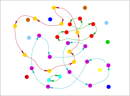
Figure 1. A typical realization of a spatial permutation. As $|\Lambda|,N\to\infty$, the jumps remain finite but the cycle lengths may diverge.

This model arises naturally from the Feynman-Kac representation of the dilute Bose gas. The jump function is then $\xi(x)=\frac{1}{4\beta}\|x\|^{2}$ (plus a normalization constant), with $\beta$ the inverse temperature of the system. Notice that if the original quantum system has periodic boundary conditions, we get the periodized Gaussian function. Cycle weights were introduced in [3] as a crude way to account for the particle interactions. But the calculations of [5] suggest that the cycle weights can be chosen so that the model describes the Bose gas exactly in the dilute regime. We do not write here the precise formula for the weights, but we observe that they satisfy the asymptotic $\alpha_{j}=-\alpha(1-O(j^{-1/5}))$, so that $\alpha_{j}$ converges as $j\to\infty$ fast enough for our purpose.

We are solely interested in properties of permutations and we introduce random variables that are functions on ${\mathcal{S}}_{N}$ rather than $\Omega_{\Lambda,N}$. Let $\ell^{(1)}(\pi),\ell^{(2)}(\pi),\dots$ denote the cycle lengths in non-increasing order, repeated with multiplicities. We will prove that, above the critical density, the cycle lengths scale like $N$ and they converge in distribution to Poisson-Dirichlet. The latter is conveniently defined using the Griffiths-Engen-McCloskey distribution GEM$(\theta)$, which is the distribution for

$$\bigl{(}\,X_{1},\,(1-X_{1})X_{2}\,,(1-X_{1})(1-X_{2})X_{3}\,,\,\dots\bigr{)},$$

where $X_{1},X_{2},\dots$ are i.i.d. beta random variables with parameter $(1,\theta)$; that is, ${\rm Prob}(X_{i}>s)=(1-s)^{\theta}$ for $0\;\leqslant\;s\;\leqslant\;1$. The Poisson-Dirichlet distribution PD$(\theta)$ is the law obtained by rearranging those numbers in non-increasing order. See [1, 14] for more information and background. In the sequel, we say that a sequence of random variables $Y^{(1)}_{n},Y^{(2)}_{n},\dots$ converges in distribution to Poisson-Dirichlet as $n\to\infty$ if, for each fixed $k$, the joint distribution of $Y^{(1)}_{n},\dots,Y^{(k)}_{n}$ converges weakly to the joint distribution of the first $k$ random variables in Poisson-Dirichlet. This is denoted

$$(Y^{(1)}_{n},Y^{(2)}_{n},\dots)\Rightarrow{\rm PD}(\theta).$$ (2.5)

As already mentioned, we make the important assumption that the jump function has nonnegative Fourier transform. This allows to define the “dispersion relation” $\varepsilon(k)$, $k\in{\mathbb{R}}^{d}$, by the equation

$$\,{\rm e}^{-\varepsilon(k)}\,=\int_{{\mathbb{R}}^{d}}\,{\rm e}^{-2\pi{\rm i}k\cdot x}\,\,{\rm e}^{-\xi(x)}\,{\rm d}x.$$ (2.6)

Notice that $\varepsilon(k)$ is real, $\varepsilon(0)=0$, and $\varepsilon(k)>0$ for all $k\neq 0$, and $\lim_{\|k\|\to\infty}\varepsilon(k)=\infty$ (by Riemann-Lebesgue). In order to avoid pathological cases we assume that $\,{\rm e}^{-\varepsilon(k)}\,$ is uniformly continuous on ${\mathbb{R}}^{d}$. We also suppose that $\varepsilon(k)\;\geqslant\;a\|k\|^{\eta}$ for small $k$, for some $a>0$ and $\eta<d$. It is easy to see that $\varepsilon(k)$ is always greater than $a\|k\|^{2}$ for small $k$, so the latter assumption always holds in dimensions $d>2$. Among possible jump functions other than Gaussians, let us mention $\,{\rm e}^{-\xi(x)}\,={\rm const}\,(|x|+1)^{-\gamma}$ with $1<\gamma<2$ in $d=1$, for which $\eta=\gamma-1$. As for the cycle weights, we consider three cases:

• $\lim_{j\to\infty}\alpha_{j}=\alpha$ with $\alpha>0$, and $\sum_{j}|\alpha_{j}-\alpha|<\infty$.

• $\lim_{j\to\infty}\alpha_{j}=\alpha$ with $\alpha\;\leqslant\;0$, and $\sum_{j}\frac{1}{j}|\alpha_{j}-\alpha|<\infty$.

• $\alpha_{j}=\gamma\log j$ with $\gamma>0$.

We now introduce the fraction $\nu$ of points in infinite cycles. It is obvious that finite systems can only host finite cycles, so the definition of $\nu$ must involve the thermodynamic limit. Given a finite number $K$, let $\nu_{K}$ denote the fraction of points in cycles of length larger than $K$. Precisely,

$$\nu_{K}=\liminf_{|\Lambda|,N\to\infty}E\Bigl{(}\frac{1}{N}\sum_{i:\ell^{(i)}>K}\ell^{(i)}\Bigr{)}.$$ (2.7)

Here and in the sequel, the limit $|\Lambda|,N\to\infty$ means that both go to infinity while keeping the density $\rho=N/|\Lambda|$ fixed. This is the standard thermodynamic limit of statistical mechanics. We then define

$$\nu=\lim_{K\to\infty}\nu_{K}.$$ (2.8)

This limit exists since $(\nu_{K})$ is decreasing and bounded. Let $\bar{\nu}_{K}$ denote the $\limsup$ of (2.7). We expect that $\bar{\nu}_{K}=\nu_{K}$ but we do not prove it. On the other hand, we will prove in Section 5 that $\bar{\nu}_{K}$ also converges to $\nu$ as $K\to\infty$.

Next we introduce the critical density by

$$\rho_{\rm{c}}=\sum_{j\;\geqslant\;1}\,{\rm e}^{-\alpha_{j}}\,\int_{{\mathbb{R}}^{d}}\,{\rm e}^{-j\varepsilon(k)}\,{\rm d}k.$$ (2.9)

It follows from our assumptions that the critical density is finite. Indeed, the numbers $\,{\rm e}^{-\alpha_{j}}\,$ are bounded, so $\rho_{\rm{c}}$ is bounded by the integral of a geometric series, $\int\frac{1}{\,{\rm e}^{\varepsilon(k)}\,-1}$, which is finite.

We propose now two theorems that confirm that $\rho_{\rm{c}}$ is indeed the critical density of the model, at least in several interesting situations. The formula (2.9) is presumably valid beyond the cases treated in this article, but the precise extent of its validity is not clear. The first theorem states that macroscopic cycles occur precisely above the critical density, and that they obey the Poisson-Dirichlet law.

Theorem 2.1.

Assume that $\alpha_{j}\to\alpha$ as described above. Then

• the fraction of points in infinite cycles is given by

  $$\nu=\max\Bigl{(}0,1-\frac{\rho_{\rm{c}}}{\rho}\Bigr{)};$$

• when $\nu>0$, i.e. when $\rho>\rho_{\rm{c}}$, the cycle structure converges in distribution to Poisson-Dirichlet: As $|\Lambda|,N\to\infty$ we have

  $$\Bigl{(}\frac{\ell^{(1)}}{\nu N},\frac{\ell^{(2)}}{\nu N},\dots\Bigr{)}\Rightarrow{\rm PD}(\,{\rm e}^{-\alpha}\,).$$

Such a law was already observed in absence of spatial structure, and when the cycle weights are constant. This case is known as the Ewens distribution, see e.g. [9, 12, 1]. Results about weights that are asymptotically Ewens can be found in [16, 6]. Spatial permutations with small cycle weights, i.e. when the limit is $\alpha=0$, were studied in [4].

The second theorem concerns cycle weights that diverge logarithmically — it is somehow the limit $\alpha\to\infty$ of Theorem 2.1. Cycle weights have a striking effect as a single giant cycle occurs above the critical density! This is in accordance with a similar observation for non-spatial permutations [6].

Theorem 2.2.

Assume that $\alpha_{j}=\gamma\log j$ with $\gamma>0$. Then

• the fraction of points in infinite cycles is given by

  $$\nu=\max\Bigl{(}0,1-\frac{\rho_{\rm{c}}}{\rho}\Bigr{)};$$

• when $\nu>0$, i.e. when $\rho>\rho_{\rm{c}}$, there is a single giant cycle that contains almost all points in infinite cycles: As $|\Lambda|,N\to\infty$ we have

  $$\frac{\ell^{(1)}}{\nu N}\Rightarrow 1.$$

The rest of this article is devoted to the proof of the results above. We reformulate the problem in the Fourier space in Section 3, following Sütő [20]. The model involves a measure on occupation numbers of Fourier modes, and of random permutations of those numbers. In Section 4 we obtain information about occupation numbers using techniques of Buffet and Pulé [8], and using certain estimates of our recent joint work with Velenik [6]. Random permutations within each mode involve the cycle weights and are thus similar to those studied in [6]. Combining all those results allows us to prove Theorems 2.1 and 2.2 in Section 5.

3. Random permutations and Fourier modes

The goal of this section is to introduce an alternative model of random permutations that involves Fourier modes, and that has the same marginal distribution on cycle lengths. Let $\Lambda^{*}=\frac{1}{L}{\mathbb{Z}}^{d}$ be the space dual to $\Lambda$ in the sense of Fourier theory.

3.1. The marginal distribution of cycle lengths

Recall that the cycle structure of a permutation $\pi\in{\mathcal{S}}_{N}$ is the sequence of cycle lengths ${\boldsymbol{\ell}}=(\ell^{(1)},\ell^{(2)},\dots,\ell^{(m)})$, with $\ell^{(i)}\;\geqslant\;\ell^{(i+1)}$ and $\ell^{(m)}\;\geqslant\;1$; the number of cycles $m$ depends on $\pi$, $1\;\leqslant\;m\;\leqslant\;N$. Those numbers form a partition of $\{1,\dots,N\}$. Another way to write ${\boldsymbol{\ell}}$ is to introduce the occupation numbers ${\boldsymbol{r}}=(r_{1},\dots,r_{N})$, where $r_{j}=\#\{i:\ell^{(i)}=j\}$. We always have

$$\sum_{i=1}^{m}\ell^{(i)}=\sum_{j=1}^{N}jr_{j}=N.$$ (3.1)

One should not confuse the occupation numbers ${\boldsymbol{r}}$ with the occupation numbers ${\boldsymbol{n}}=(n_{k})$ to be introduced later; they are not related in any direct way.

Proposition 3.1.

The marginal of the probability measure (2.3) on occupation numbers is

$${\rm Prob}({\boldsymbol{r}})=\frac{1}{Y}\prod_{j=1}^{N}\frac{1}{r_{j}!}\Bigl{(}\frac{\,{\rm e}^{-\alpha_{j}}\,}{j}\sum_{k\in\Lambda^{*}}\,{\rm e}^{-j\varepsilon(k)}\,\Bigr{)}^{r_{j}},$$

with $Y$ the normalization of (2.4).

Proof.

The marginal probability on permutations is

$$\begin{split}{\rm Prob}(\pi)&=\frac{1}{N!Y}\int_{\Lambda^{N}}\,{\rm e}^{-H_{\Lambda}({\boldsymbol{x}},\pi)}\,{\rm d}{\boldsymbol{x}}\\ &=\frac{1}{N!Y}\int_{\Lambda^{N}}\,{\rm e}^{-\sum_{i=1}^{N}\xi_{\Lambda}(x_{i}-x_{\pi(i)})-\sum_{j\;\geqslant\;1}\alpha_{j}r_{j}(\pi)}\,{\rm d}x_{1}\dots\rm dx_{N}.\end{split}$$ (3.2)

We observe that integrals factorize according to permutation cycles. The contribution of a cycle of length $j$ is (with $y_{j+1}\equiv y_{1}$)

$${}\,{\rm e}^{-\alpha_{j}}\,\int_{\Lambda^{j}}\,{\rm e}^{-\sum_{i=1}^{j}\xi_{\Lambda}(y_{i}-y_{i+1})}\,{\rm d}y_{1}\dots\rm dy_{j}=\,{\rm e}^{-\alpha_{j}}\,|\Lambda|\sum_{z\in{\mathbb{Z}}^{d}}\bigl{(}\,{\rm e}^{-\xi}\,\bigr{)}^{*j}(Lz).$$ (3.3)

To see the equality in (3.3), we start with the right hand side. Using the definition of the convolution, writing $|\Lambda|=\int_{\Lambda}{\rm d}y_{1}$, and shifting all the variables in the convolution integrals by $y_{1}$ gives

$$\begin{split}&|\Lambda|\sum_{z\in{\mathbb{Z}}^{d}}\bigl{(}\,{\rm e}^{-\xi}\,\bigr{)}^{*j}(Lz)\\ &=\sum_{z\in{\mathbb{Z}}^{d}}\int_{\Lambda}{\rm d}y_{1}\int_{{\mathbb{R}}^{d(j-1)}}{\rm d}y_{2}\dots\rm dy_{j}\,{\rm e}^{-\xi(Lz-y_{2}+y_{1})}\,\,{\rm e}^{-\xi(y_{2}-y_{3})}\,\dots\,{\rm e}^{-\xi(y_{j}-y_{1})}\,\\ &=\sum_{z_{1}\in{\mathbb{Z}}^{d}}\int_{\Lambda}{\rm d}y_{1}\sum_{z_{2},\ldots,z_{j}\in{\mathbb{Z}}^{d}}\int_{\Lambda^{j-1}}{\rm d}y_{2}\dots\rm dy_{j}\,{\rm e}^{-\xi(y_{1}-y_{2}+L(z_{1}-z_{2}))}\,\,{\rm e}^{-\xi(y_{2}-y_{3}+L(z_{2}-z_{3}))}\,\\ &\hskip 113.81102pt\dots\,{\rm e}^{-\xi(y_{j-1}-y_{j}+L(z_{j-1}-z_{j}))}\,-\,{\rm e}^{-\xi(y_{j}-y_{1}+Lz_{j})}\,.\end{split}$$ (3.4)

The last equality is obtained by decomposing the domain of integration ${\mathbb{R}}^{d}$ into cubes $\Lambda+Lz$ with $z\in{\mathbb{Z}}^{d}$ and then changing variables in the integrals so that all the boxes become centered at $0$. We now change to summation index: $\tilde{z}_{j}=z_{j}$, and $\tilde{z}_{i}=z_{i}-z_{i+1}$ for $i<j$. It is easy to see that this is indeed a bijection on $({\mathbb{Z}}^{d})^{j}$. Summing over $\tilde{z}_{i}$ instead of $z_{i}$ now gives the left hand side of (3.3).

The Fourier transform of $(\,{\rm e}^{-\xi}\,)^{*j}$ is $\,{\rm e}^{-j\varepsilon(k)}\,$. The Poisson summation formula states that

$$\sum_{z\in{\mathbb{Z}}^{d}}f(Lz)=\frac{1}{|\Lambda|}\sum_{k\in\Lambda^{*}}\widehat{f}(k),$$ (3.5)

where $\widehat{f}$ is the Fourier transform of $f$, whose precise definition can be found in Eq. (2.6). We then get

$${\rm Prob}(\pi)=\frac{1}{N!Y}\prod_{j=1}^{N}\Bigl{(}\,{\rm e}^{-\alpha_{j}}\,\sum_{k\in\Lambda^{*}}\,{\rm e}^{-j\varepsilon(k)}\,\Bigr{)}^{r_{j}(\pi)}.$$ (3.6)

All permutations of a given cycle structure have the same probability, and there are

$$\frac{N!}{\prod_{j}j^{r_{j}}r_{j}!}$$ (3.7)

elements in the cycle structure defined by ${\boldsymbol{r}}$. We get the claim by multiplying the above probability by this number. ∎

3.2. Decomposition of permutations according to Fourier modes

We denote by ${\boldsymbol{n}}=(n_{k})$ the occupation numbers indexed by $k\in\Lambda^{*}$, and by ${\mathcal{N}}_{\Lambda,N}$ the set of occupation numbers such that $\sum_{k\in\Lambda^{*}}n_{k}=N$. Next, we introduce permutations that are also indexed by Fourier modes, ${\boldsymbol{\pi}}=(\pi_{k})$. Let ${\mathcal{M}}_{\Lambda,N}$ be the set of pairs $({\boldsymbol{n}},{\boldsymbol{\pi}})$ where ${\boldsymbol{n}}\in{\mathcal{N}}_{\Lambda,N}$ and ${\boldsymbol{\pi}}=(\pi_{k})$ with $\pi_{k}\in{\mathcal{S}}_{n_{k}}$ for each $k\in\Lambda^{*}$. We introduce a probability measure on ${\mathcal{N}}_{\Lambda,N}$:

$${\rm Prob}({\boldsymbol{n}})=\frac{1}{Y}\prod_{k\in\Lambda^{*}}\,{\rm e}^{-\varepsilon(k)n_{k}}\,h_{n_{k}}$$ (3.8)

with

$$h_{n}=\frac{1}{n!}\sum_{\pi\in{\mathcal{S}}_{n}}\,{\rm e}^{-\sum_{j\;\geqslant\;1}\alpha_{j}r_{j}(\pi)}\,,$$ (3.9)

and $h_{0}=1$. We will check later that the normalization $Y$ is the same as given in (2.4). Then we introduce the probability of a pair $({\boldsymbol{n}},{\boldsymbol{\pi}})$ by

$${\rm Prob}({\boldsymbol{n}},{\boldsymbol{\pi}})=\frac{1}{Y}\prod_{k\in\Lambda^{*}}\frac{1}{n_{k}!}\,{\rm e}^{-\varepsilon(k)n_{k}-\sum_{j\;\geqslant\;1}\alpha_{j}r_{j}(\pi_{k})}\,.$$ (3.10)

Notice that (3.8) is the marginal of (3.10) with respect to ${\boldsymbol{\pi}}$. The conditional probability ${\rm Prob}({\boldsymbol{\pi}}|{\boldsymbol{n}})$, where $\pi_{k}\in{\mathcal{S}}_{n_{k}}$ for all $k$, is given by

$${\rm Prob}({\boldsymbol{\pi}}|{\boldsymbol{n}})=\prod_{k\in\Lambda^{*}}\Bigl{(}\frac{1}{n_{k}!h_{n_{k}}}\,{\rm e}^{-\sum_{j\;\geqslant\;1}\alpha_{j}r_{j}(\pi_{k})}\,\Bigr{)}.$$ (3.11)

That is, given ${\boldsymbol{n}}$, each $\pi_{k}$ is independent and distributed as nonspatial random permutations with cycle weights (see Eq. (5.1) below). Given ${\boldsymbol{\pi}}$, let $r_{j}=\sum_{k}r_{j}(\pi_{k})$.

Proposition 3.2.

The marginal of the probability measure (3.10) with respect to ${\boldsymbol{r}}$ is identical to the marginal of the probability measure (2.3).

Proof.

We check that the marginal of (3.10) gives the formula of Proposition 3.1. For this, let ${\boldsymbol{r}}$ be a collection of occupation numbers, and write $(r_{jk}):{\boldsymbol{r}}$ for the set of all integers $r_{jk}$ ($j\;\geqslant\;1,k\in\Lambda^{\ast}$) such that $\sum_{k}r_{jk}=r_{j}$ for all $j$. Then,

$$\begin{split}{\rm Prob}({\boldsymbol{r}})&=\frac{1}{Y}\sum_{(r_{jk}):{\boldsymbol{r}}}\,\,\sum_{\begin{subarray}{c}({\boldsymbol{n}},{\boldsymbol{\pi}}):\\ r_{j}(\pi_{k})=r_{jk}\end{subarray}}\prod_{k\in\Lambda^{*}}\Bigl{(}\frac{1}{n_{k}!}\,{\rm e}^{-\varepsilon(k)n_{k}-\sum_{j}\alpha_{j}r_{j}(\pi_{k})}\,\Bigr{)}\\ &=\frac{1}{Y}\sum_{(r_{jk}):{\boldsymbol{r}}}\prod_{k\in\Lambda^{*}}\Bigl{(}\frac{1}{\prod_{j}j^{r_{jk}}r_{jk}!}\,{\rm e}^{-\varepsilon(k)\sum_{j}jr_{jk}-\sum_{j}\alpha_{j}r_{jk}}\,\Bigr{)}.\end{split}$$ (3.12)

We have summed over $\pi_{k}$ that are compatible with $r_{jk}$, using the formula (3.7) for the number of elements. The bracket above factorizes according to $j$. Using

$$\prod_{k\in\Lambda^{*}}\frac{\,{\rm e}^{-\alpha_{j}r_{jk}}\,}{j^{r_{jk}}}=\Bigl{(}\frac{\,{\rm e}^{-\alpha_{j}}\,}{j}\Bigr{)}^{r_{j}},$$ (3.13)

and writing, for fixed $j\;\geqslant\;1$, $(r_{jk}):r_{j}$ for the set of integers $r_{jk}$ with $\sum_{k}r_{jk}=r_{j}$, we get

$${\rm Prob}({\boldsymbol{r}})=\frac{1}{Y}\prod_{j\;\geqslant\;1}\biggl{[}\Bigl{(}\frac{\,{\rm e}^{-\alpha_{j}}\,}{j}\Bigr{)}^{r_{j}}\sum_{(r_{jk}):r_{j}}\prod_{k\in\Lambda^{*}}\frac{1}{r_{jk}!}\,{\rm e}^{-j\varepsilon(k)r_{jk}}\,\biggr{]}.$$ (3.14)

For each fixed $j$, the multinomial theorem gives

$$\sum_{(r_{jk}):r_{j}}\prod_{k\in\Lambda^{*}}\frac{\,{\rm e}^{-j\varepsilon(k)r_{jk}}\,}{r_{jk}!}=\frac{1}{r_{j}!}\Bigl{(}\sum_{k\in\Lambda^{*}}\,{\rm e}^{-j\varepsilon(k)}\,\Bigr{)}^{r_{j}}.$$ (3.15)

Then ${\rm Prob}({\boldsymbol{r}})$ is indeed given by the formula of Proposition 3.1. This also proves that $Y$ is the correct normalization that makes (3.8) and (3.10) probability measures. ∎

4. Properties of occupation numbers

We study in this section the probability measure of occupation numbers of Fourier modes, ${\rm Prob}({\boldsymbol{n}})$, that is defined in (3.8). We show that the typical ${\boldsymbol{n}}$ has the following properties:

• $\frac{n_{0}}{N}=\max(0,1-\frac{\rho_{\rm{c}}}{\rho})$;

• $\frac{1}{N}\sum_{0<\|k\|<\delta}n_{k}$ is small when $\delta$ is small.

• For all $\delta>0$, $\frac{1}{N}\sum_{\|k\|\;\geqslant\;\delta}n_{k}1_{n_{k}>M}$ is small when $M$ is large.

The behavior of the normalizations $h_{n}$ defined in (3.9) play an important rôle. We assume that $h_{n}$ grows or vanishes at most polynomially, i.e., there are constants $C$ and $\kappa$ such that for all $n\;\geqslant\;1$,

$$(Cn)^{-\kappa}\;\leqslant\;h_{n}\;\leqslant\;(Cn)^{\kappa}.$$ (4.1)

We also need that certain ratios of $h_{n}$ be bounded. Precisely, for $s>1$, let

$$C(s)=\sup_{\begin{subarray}{c}m,n\;\geqslant\;1\\ n/s<m<sn\end{subarray}}\frac{h_{m}}{h_{n}}.$$ (4.2)

We assume that $C(s)$ is finite for any $s$.

Those properties have been verified in [6] when $\alpha_{j}\to\alpha$ and $\alpha_{j}=\gamma\log j$. Indeed, one finds $h_{n}\sim n^{-r}$, with $r=\,{\rm e}^{-\alpha}\,-1$ in the first case and $r=-1-\gamma$ in the second case. The results of the present article actually extend to other cycle weights, as long as Eqs (4.1) and (4.2) hold true.

The radius of convergence of the generating function of $h_{n}$ is equal to 1. We have the following identity for all $\gamma>0$:

$$\sum_{n\;\geqslant\;0}\,{\rm e}^{-\gamma n}\,h_{n}=\exp\sum_{j\;\geqslant\;1}\tfrac{1}{j}\,{\rm e}^{-\gamma j-\alpha_{j}}\,.$$ (4.3)

See [4, 16] for the proof.

4.1. Macroscopic occupation of the zero mode

We use a strategy that is inspired by Buffet and Pulé in their study of the ideal Bose gas [8]. It consists in looking at the Laplace transform of the distribution of $\frac{n_{0}}{N}$. Let $Y(N)$ be the normalization of Eq. (2.4). We now put the explicit dependence on $N$ because it is going to vary. Notice that $Y(N)$ also depends on $\Lambda$, but the domain is fixed throughout.

We have

$${\rm Prob}(n_{0}=j)=\frac{h_{j}}{Y(N)}\sum_{\begin{subarray}{c}{\boldsymbol{n}}\in{\mathcal{N}}_{\Lambda,N}\\ n_{0}=j\end{subarray}}\prod_{k\neq 0}\,{\rm e}^{-\varepsilon(k)n_{k}}\,h_{n_{k}}=h_{j}\frac{\check{Y}(N-j)}{Y(N)},$$ (4.4)

with

$$\check{Y}(N)=\sum_{\begin{subarray}{c}{\boldsymbol{n}}\in{\mathcal{N}}_{\Lambda,N}\\ n_{0}=0\end{subarray}}\prod_{k\in\Lambda^{*}}\,{\rm e}^{-\varepsilon(k)n_{k}}\,h_{n_{k}}.$$ (4.5)

Notice the relation

$$Y(N)=\sum_{j=0}^{N}h_{j}\check{Y}(N-j).$$ (4.6)

We are often going to interchange infinite sums and products. Let ${\mathcal{N}}$ be the set of finite sequences of integers. Notice that ${\mathcal{N}}$ is countably infinite. The following lemma is easy to prove and sufficient for our purpose.

Lemma 4.1.

Let $a(k,n)$ be a nonnegative function such that $a(k,0)=1$ for all $k$. Then

$$\sum_{{\boldsymbol{n}}\in{\mathcal{N}}}\prod_{k\;\geqslant\;1}a(k,n_{k})=\prod_{k\;\geqslant\;1}\Big{(}\sum_{n\;\geqslant\;0}a(k,n)\Big{)}.$$

(It is possible that both sides are infinite.)

Proof.

Let $\ell({\boldsymbol{n}})$ be the index of the largest nonzero integer in ${\boldsymbol{n}}$. For every $m\;\geqslant\;1$ we have

$$\sum_{{\boldsymbol{n}}\in{\mathcal{N}}:\ell({\boldsymbol{n}})\;\leqslant\;m}\prod_{k=1}^{\ell({\boldsymbol{n}})}a(k,n_{k})=\sum_{n_{1},\dots,n_{m}\;\geqslant\;0}\prod_{k=1}^{m}a(k,n_{k})=\prod_{k=1}^{m}\Bigl{(}\sum_{n\;\geqslant\;0}a(k,n)\Bigr{)}.$$ (4.7)

The left hand side and the right hand side are clearly increasing in $m$, and we obtain the lemma by letting $m\to\infty$. ∎

Lemma 4.1 also holds for complex $a(k,n)$ under the assumption $\sum_{k\;\geqslant\;0}\sum_{n\;\geqslant\;1}|a(k,n)|$ be finite. This can be proved using dominated convergence, but it is not needed here.

We introduce a Riemann approximation to the critical density (2.9) which will be useful in Proposition 4.3 below.

$$\rho_{\rm{c}}^{(\Lambda)}=\sum_{j\;\geqslant\;1}\,{\rm e}^{-\alpha_{j}}\,\frac{1}{|\Lambda|}\sum_{k\neq 0}\,{\rm e}^{-j\varepsilon(k)}\,.$$ (4.8)

Lemma 4.2.

$\lim_{|\Lambda|\to\infty}\rho_{\rm c}^{(\Lambda)}=\rho_{\rm c}$.

Proof.

Since $\,{\rm e}^{-\varepsilon(k)}\,$ is uniformly continuous, the Riemann sum $|\Lambda|^{-1}\sum_{k\neq 0}\,{\rm e}^{-j\varepsilon(k)}\,$ converges to $\int\,{\rm e}^{-j\varepsilon(k)}\,\,{\rm d}k$ for each $j$. We need to show that the limit $|\Lambda|\to\infty$ can be interchanged with the sum over $j$ and we use dominated convergence. We sum separately over $\|k\|\;\leqslant\;1$ and $\|k\|>1$. For $\|k\|>1$ we use $\varepsilon(k)>c>0$, so that

$$\frac{1}{|\Lambda|}\sum_{\|k\|>1}\,{\rm e}^{-j\varepsilon(k)}\,\;\leqslant\;\,{\rm e}^{-jc/2}\,\frac{1}{|\Lambda|}\sum_{k\in\Lambda^{\ast}}\,{\rm e}^{-\varepsilon(k)}\,$$ (4.9)

for $j\;\geqslant\;2$. The latter sum is easily seen to converge using Eq. (3.5), so the right hand side is bounded by $C\,{\rm e}^{-jc/2}\,$, which is summable. For $\|k\|\;\leqslant\;1$, we use $\varepsilon(k)>a\|k\|^{\eta}$ with $a>0$. Since $\,{\rm e}^{-ja\|k\|^{\eta}}\,$ is decreasing, we can estimate it with integrals, namely

$$\begin{split}\frac{1}{|\Lambda|}\sum_{k\neq 0,\|k\|\;\leqslant\;1}\,{\rm e}^{-j\varepsilon(k)}\,&\;\leqslant\;\frac{1}{|\Lambda|}\sum_{k\neq 0}\,{\rm e}^{-aj\|k\|^{\eta}}\,\\ &\;\leqslant\;2^{d}\int_{{\mathbb{R}}^{d}}\,{\rm e}^{-aj\|k\|^{\eta}}\,{\rm d}k=\frac{2^{d}d\pi^{d/2}\Gamma(\frac{d}{\eta})}{\Gamma(\frac{d}{2}+1)\eta(aj)^{d/\eta}}.\end{split}$$ (4.10)

The only relevant term in the upper bound is $j^{-d/\eta}$, which makes the sum over $j$ summable in Eq. (4.8). The claim follows from the dominated convergence theorem. ∎

Let ${\mathcal{N}}_{\Lambda}=\cup_{N\;\geqslant\;0}{\mathcal{N}}_{\Lambda,N}$ be the set of occupation numbers on $\Lambda^{*}$ where $\sum_{k}n_{k}$ is an arbitrary finite number. Using Lemma 4.1 we find

$$\begin{split}\check{Z}&=\sum_{N\;\geqslant\;0}\check{Y}(N)=\sum_{\begin{subarray}{c}{\boldsymbol{n}}\in{\mathcal{N}}_{\Lambda}\\ n_{0}=0\end{subarray}}\prod_{k\in\Lambda^{*}}\,{\rm e}^{-\varepsilon(k)n_{k}}\,h_{n_{k}}\\ &=\prod_{k\neq 0}\Bigl{(}\sum_{n\;\geqslant\;0}\,{\rm e}^{-\varepsilon(k)n}\,h_{n}\Bigr{)}=\exp\Bigl{(}\sum_{j\;\geqslant\;1}\tfrac{1}{j}\,{\rm e}^{-\alpha_{j}}\,\sum_{k\neq 0}\,{\rm e}^{-j\varepsilon(k)}\,\Bigr{)}.\end{split}$$ (4.11)

The last identity follows from (4.3) since $\inf_{k\neq 0}\varepsilon(k)=c(\Lambda)>0$. $\check{Z}$ is finite by Lemma 4.2. This allows to introduce the following probability measure on $[0,\infty)$:

$$\mu_{\Lambda}=\frac{1}{\check{Z}}\sum_{N\;\geqslant\;0}\check{Y}(N)\delta_{N/|\Lambda|}.$$ (4.12)

The motivation for $\mu_{\Lambda}$ is that the distribution of the occupation of the zero mode can be expressed as

$$\begin{split}{\rm Prob}(\tfrac{n_{0}}{N}\;\geqslant\;a)&=\sum_{j=\lceil aN\rceil}^{N}h_{j}\frac{\check{Y}(N-j)}{Y(N)}=\sum_{j=0}^{\lfloor(1-a)N\rfloor}h_{N-j}\frac{\check{Y}(j)}{Y(N)}\\ &=\frac{\int_{0}^{(1-a)\rho}h(|\Lambda|(\rho-s))\,{\rm d}\mu_{\Lambda}(s)}{\int_{0}^{\rho}h(|\Lambda|(\rho-s))\,{\rm d}\mu_{\Lambda}(s)}.\end{split}$$ (4.13)

Here $h(x)$ can be any function interpolating the values $h_{n}$ at $n\in{\mathbb{N}}$, e.g. linear interpolation. We use the notation purely for convenience and will never evaluate $h(x)$ at non-integer points.

We now have all the elements that allow to state and to prove the key properties leading to the macroscopic occupation of the zero Fourier mode.

Proposition 4.3.

• $\mu_{\Lambda}\to\delta_{\rho_{\rm{c}}}$ weakly as $|\Lambda|\to\infty$.

• Let $\lambda(\Lambda)\in{\mathbb{R}}$ such that $|\lambda(\Lambda)|\;\leqslant\;|\Lambda|^{\frac{1-\eta/d}{2}}$, then

  $$E_{\mu_{\Lambda}}\bigl{(}\,{\rm e}^{\lambda(\Lambda)(X-\rho_{\rm{c}}^{(\Lambda)})}\,\bigr{)}\to 1.$$

The parameter $\eta$ in the claim (b) is the one that appears in the condition for $\varepsilon(k)$, see the paragraph after Eq. (2.6). The relevant aspect of the claim (b) is that the expectation is bounded uniformly in the domain even though $\lambda(\Lambda)$ diverges. Markov’s inequality then gives the following concentration property for $|\Lambda|$ large enough, which will be used later:

$$\begin{split}{\rm Prob}_{\mu_{\Lambda}}(|X-\rho_{\rm{c}}|>\epsilon)&\;\leqslant\;\,{\rm e}^{-\epsilon|\Lambda|^{\frac{1-\eta/d}{2}}}\,E_{\mu_{\Lambda}}\Bigl{(}\,{\rm e}^{|\Lambda|^{\frac{1-\eta/d}{2}}(X-\rho_{\rm{c}}^{(\Lambda)})}\,+\,{\rm e}^{-|\Lambda|^{\frac{1-\eta/d}{2}}(X-\rho_{\rm{c}}^{(\Lambda)})}\,\Bigr{)}\\ &\;\leqslant\;3\,{\rm e}^{-\epsilon|\Lambda|^{\frac{1-\eta/d}{2}}}\,.\end{split}$$ (4.14)

Proof of Proposition 4.3.

(a) follows from (b), see (4.14). For (b) we note that $a(k,n)=\,{\rm e}^{-(\varepsilon(k)-\lambda(\Lambda)/|\Lambda|)n}\,h_{n}$ fulfils the assumptions of Lemma 4.1, and thus

$$\begin{split}E_{\mu_{\Lambda}}(\,{\rm e}^{\lambda(\Lambda)X}\,)&=\int_{0}^{\infty}\,{\rm e}^{\lambda(\Lambda)s}\,{\rm d}\mu_{\Lambda}(s)=\frac{1}{\check{Z}}\sum_{N\;\geqslant\;0}\check{Y}(N)\,{\rm e}^{\lambda(\Lambda)N/|\Lambda|}\,\\ &=\frac{1}{\check{Z}}\sum_{\begin{subarray}{c}{\boldsymbol{n}}\in{\mathcal{N}}_{\Lambda}\\ n_{0}=0\end{subarray}}\prod_{k\neq 0}\,{\rm e}^{-(\varepsilon(k)-\lambda(\Lambda)/|\Lambda|)n_{k}}\,h_{n_{k}}\end{split}$$ (4.15)

Since $\inf_{k\neq 0}\varepsilon(k)-\lambda(\Lambda)/|\Lambda|>0$, (4.3) applies, and together with (4.11) we obtain

$$E_{\mu_{\Lambda}}(\,{\rm e}^{\lambda(\Lambda)X}\,)=\exp\Bigl{(}\sum_{j\;\geqslant\;1}\tfrac{1}{j}\,{\rm e}^{-\alpha_{j}}\,\sum_{k\neq 0}\,{\rm e}^{-j\varepsilon(k)}\,(\,{\rm e}^{j\lambda(\Lambda)/|\Lambda|}\,-1)\Bigr{)}$$ (4.16)

By (4.8) and rearranging, we get

$$E_{\mu_{\Lambda}}\bigl{(}\,{\rm e}^{\lambda(\Lambda)(X-\rho_{\rm{c}}^{(\Lambda)})}\,\bigr{)}=\exp\Bigl{(}\sum_{j\;\geqslant\;1}\tfrac{1}{j}\,{\rm e}^{-\alpha_{j}}\,\sum_{k\neq 0}\,{\rm e}^{-j\varepsilon(k)}\,\bigl{(}\,{\rm e}^{j\lambda(\Lambda)/|\Lambda|}\,-1-j\tfrac{\lambda(\Lambda)}{|\Lambda|}\bigr{)}\Bigr{)}.$$ (4.17)

We show that the exponent vanishes as $|\Lambda|\to\infty$ using dominated convergence. We use $|\,{\rm e}^{x}\,-1-x|\;\leqslant\;\frac{1}{2}x^{2}\,{\rm e}^{|x|}\,$ (which is easy to check using Taylor series) with $x=j\lambda(\Lambda)/|\Lambda|$. The exponent in the right hand side of (4.17) is bounded, in absolute value, by

$$\tfrac{1}{2}\sum_{j\;\geqslant\;1}\,{\rm e}^{-\alpha_{j}}\,\frac{1}{|\Lambda|}\sum_{k\neq 0}\,{\rm e}^{-\frac{1}{2}j\varepsilon(k)}\,\Bigl{[}\tfrac{j\lambda^{2}(\Lambda)}{|\Lambda|}\,{\rm e}^{-j(\frac{1}{2}\varepsilon(k)-|\lambda(\Lambda)|/|\Lambda|)}\,\Bigr{]}.$$ (4.18)

Since $\varepsilon(k)\;\geqslant\;a|\Lambda|^{-\eta/d}$ and $|\lambda(\Lambda)|^{2}\;\leqslant\;|\Lambda|^{1-\eta/d}$, the bracket is bounded above uniformly in $j$ for all $|\Lambda|$ large enough. The sum over $k$ has been estimated in (4.9) and (4.10). Since $\sum_{j}\,{\rm e}^{-\alpha_{j}}\,j^{-d/\eta}<\infty$, we can interchange the limit $|\Lambda|\to\infty$ and the sum over $j$ by dominated convergence. The bracket in (4.18) tends to 0 as $|\Lambda|\to\infty$, for all fixed $j$. It follows that (4.18) converges to zero and (4.17) converges to one. ∎

Proposition 4.4.

Suppose that $\rho>\rho_{\rm{c}}$. Then, in the thermodynamic limit $|\Lambda|,N\to\infty$,

$${\rm Prob}(\tfrac{n_{0}}{N}>a)\to\begin{cases}1&\text{if }a<1-\frac{\rho_{\rm{c}}}{\rho},\\ 0&\text{if }a>1-\frac{\rho_{\rm{c}}}{\rho}.\end{cases}$$

Proof.

We show that, for every $\epsilon>0$,

$${\rm Prob}\bigl{(}\bigl{|}\tfrac{n_{0}}{N}-\tfrac{\rho-\rho_{\rm c}}{\rho}\bigr{|}>\epsilon\bigr{)}\to 0.$$ (4.19)

Using the expression (4.12) which involves the measure $\mu_{\Lambda}$, we write the probability as

$${\rm Prob}\bigl{(}\bigl{|}\tfrac{n_{0}}{N}-\tfrac{\rho-\rho_{\rm c}}{\rho}\bigr{|}>\epsilon\bigr{)}=\frac{J_{-}+J_{+}}{J_{-}+J_{0}+J_{+}},$$ (4.20)

with

$$\begin{split}&J_{-}=\int_{0}^{\rho_{\rm c}-\epsilon\rho}\frac{h(|\Lambda|(\rho-s))}{h(|\Lambda|(\rho-\rho_{\rm c}))}{\rm d}\mu_{\Lambda}(s),\\ &J_{0}=\int_{\rho_{\rm c}-\epsilon\rho}^{\rho_{\rm c}+\epsilon\rho}\frac{h(|\Lambda|(\rho-s))}{h(|\Lambda|(\rho-\rho_{\rm c}))}{\rm d}\mu_{\Lambda}(s),\\ &J_{+}=\int_{\rho_{\rm c}+\epsilon\rho}^{\rho}\frac{h(|\Lambda|(\rho-s))}{h(|\Lambda|(\rho-\rho_{\rm c}))}{\rm d}\mu_{\Lambda}(s).\end{split}$$ (4.21)

By (4.2), the ratios of $h(\cdot)$ are bounded above and below for all $0<s<\rho-c$ uniformly in $\Lambda$. This shows that $J_{-}\to 0$ and that $J_{0}$ is bounded away from 0 as $|\Lambda|\to\infty$. As for $J_{+}$, we need to be careful with the integration over $s$ close to $\rho$. By (4.1), the ratio in $J_{+}$ is bounded by

$$\frac{h(|\Lambda|(\rho-s))}{h(|\Lambda|(\rho-\rho_{\rm c}))}\;\leqslant\;\epsilon^{\kappa}(C|\Lambda|\rho)^{2\kappa},$$ (4.22)

which is valid provided $|\Lambda|\epsilon\;\geqslant\;1$. Then

$$J_{+}\;\leqslant\;\epsilon^{\kappa}(C|\Lambda|\rho)^{2\kappa}E_{\mu_{\Lambda}}(1_{s>\rho_{\rm c}+\epsilon\rho}),$$ (4.23)

and it goes to zero by Eq. (4.14). ∎

4.2. No macroscopic occupation below the critical density

For $\rho<\rho_{\rm{c}}$, the support of the Dirac measure to which the measures $\mu_{\Lambda}$ converge lies outside of the interval $[0,\rho]$, and the above argument fails. In its place, we use the formula

$${\rm Prob}(n_{0}\;\geqslant\;j)=\frac{1}{Y(N)}\sum_{\begin{subarray}{c}{\boldsymbol{n}}\in{\mathcal{N}}_{\Lambda,N}\\ n_{0}\;\geqslant\;j\end{subarray}}\,\,\prod_{k\in\Lambda^{\ast}}\,{\rm e}^{-n_{k}\varepsilon(k)}\,h_{n_{k}}=\frac{Y(N-j,j)}{Y(N)},$$ (4.24)

where

$$Y(m,j)=\sum_{{\boldsymbol{n}}\in{\mathcal{N}}_{\Lambda,m}}\frac{h_{n_{0}+j}}{h_{n_{0}}}\prod_{k\in\Lambda^{\ast}}\,{\rm e}^{-n_{k}\varepsilon(k)}\,h_{n_{k}}.$$ (4.25)

We apply summation by parts $E(f(X))=f(0)+\sum_{j=1}^{N}\big{[}f(j)-f(j-1)\big{]}P(X\;\geqslant\;j)$ to the function $\,{\rm e}^{-\lambda n_{0}/N}\,$, and we find

$$\begin{split}E(\,{\rm e}^{-\lambda n_{0}/N}\,)&=1+\frac{(1-\,{\rm e}^{\lambda/N}\,)}{Y(N)}\sum_{j=1}^{N}\,{\rm e}^{-\lambda j/N}\,Y(N-j,j)\\ &=1+\frac{\,{\rm e}^{-\lambda}\,(1-\,{\rm e}^{\lambda/N}\,)}{Y(N)}\sum_{j=0}^{N-1}\,{\rm e}^{\lambda j/N}\,Y(j,N-j).\end{split}$$ (4.26)

For the last equality, we used a change of summation index $j\to N-j$.

Proposition 4.5.

Suppose that $\rho\;\leqslant\;\rho_{\rm{c}}$. In the thermodynamic limit $|\Lambda|$, $N\to\infty$,

$${\rm Prob}(\tfrac{n_{0}}{N}>\delta)\to 0.$$

for all $\delta>0$.

Proof.

By (4.26),

$$|E(\,{\rm e}^{\frac{\lambda n_{0}}{N}}\,)-1|\;\leqslant\;\frac{{\rm const}}{N}\left(\sum_{j=0}^{(1-\epsilon)N}\frac{Y(j,N-j)}{Y(N)}+\sum_{j=(1-\epsilon)N}^{N-1}\frac{Y(j,N-j)}{Y(N)}\right).$$ (4.27)

From (4.24) it is obvious that $\frac{Y(j,N-j)}{Y(N)}\;\leqslant\;1$, as it is equal to ${\rm Prob}(n_{0}\;\geqslant\;N-j)$. Thus the second term above, along with the prefactor $1/N$, is bounded by ${\rm const}\epsilon$. For the first term, we use the inequality

$$\sup_{r}\frac{h_{r+j}}{h_{r}}\;\leqslant\;C_{0}(1+j)^{2\kappa}$$ (4.28)

for some constant $C_{0}$; this follows from (4.1) and (4.2). Then, $Y(N,j)\;\leqslant\;Y(N)C_{0}(1+j)^{2\kappa}$, and

$$\sum_{j=0}^{\lfloor(1-\epsilon)N\rfloor}\frac{Y(j,N-j)}{Y(N)}\;\leqslant\;C_{0}\sum_{j=0}^{\lfloor(1-\epsilon)N\rfloor}\frac{Y(j)}{Y(N)}(N-j+1)^{2\kappa}$$ (4.29)

Now

$$\frac{Y(j)}{Y(N)}=\,{\rm e}^{-|\Lambda|(q_{\Lambda}(j/|\Lambda|)-q_{\Lambda}(\rho))}\,,$$ (4.30)

where $q_{\Lambda}(\rho)=-\frac{1}{|\Lambda|}\log Y(|\Lambda|\rho)$ is the finite volume free energy associated with the partition function $Y$. It was shown in [4], under conditions on the coefficients $\alpha_{j}$ that are more general than the present ones, that $q_{\Lambda}$ converges uniformly on compact intervals to a convex function $q$, and that $\rho\mapsto q(\rho)$ is strictly decreasing for $\rho<\rho_{\rm{c}}$. Thus for each $\epsilon>0$ there is $b_{\epsilon}>0$ such that $q_{\Lambda}(j/|\Lambda|)-q_{\Lambda}(\rho)>b_{\epsilon}$ for all $|\Lambda|$ large enough, and all $j\;\leqslant\;(1-\epsilon)N$. So

$$\sum_{j=0}^{\lfloor(1-\epsilon)N\rfloor}\frac{Y(j,N-j)}{Y(N)}\;\leqslant\;C_{0}\,{\rm e}^{-b_{\epsilon}|\Lambda|}\,\sum_{j=0}^{\lfloor(1-\epsilon)N\rfloor}(N-j+1)^{2\kappa}\;\leqslant\;C_{0}\,{\rm e}^{-b_{\epsilon}N/\rho}\,N^{2\kappa+1},$$ (4.31)

which converges to zero as $N\to\infty$. Since $\epsilon$ was arbitrary, we have shown that $E(\,{\rm e}^{\lambda n_{0}/N}\,)\to 1$ for all $\lambda>0$, which implies the claim. ∎

4.3. Occupation of nonzero modes

We now turn to the modes $k\neq 0$. Recall the bound $C(s)$ for the ration of $h_{n}$ in Eq. (4.2).

Lemma 4.6.

For $0<\sigma<1$, $k\in\Lambda^{\ast}$, and $j\;\geqslant\;0$, we have

$${\rm Prob}(n_{k}\;\geqslant\;j)\;\leqslant\;C(\tfrac{1}{\sigma})^{2}\,{\rm e}^{-j(1-\sigma)\varepsilon(k)}\,.$$

Proof.

Using (4.2), we have

$$\begin{split}{\rm Prob}&(n_{k}\;\geqslant\;j)=\frac{1}{Y(N)}\sum_{\begin{subarray}{c}{\boldsymbol{n}}\in{\mathcal{N}}_{\Lambda,N}\\ n_{k}\;\geqslant\;j\end{subarray}}\prod_{k^{\prime}\in\Lambda^{\ast}}\,{\rm e}^{-n_{k^{\prime}}\varepsilon(k^{\prime})}\,h_{n_{k^{\prime}}}\\ &=\frac{1}{Y(N)}\sum_{\begin{subarray}{c}{\boldsymbol{n}}\in{\mathcal{N}}_{\Lambda,N-(1-\sigma)j}\\ n_{k}\;\geqslant\;\sigma j\end{subarray}}\,{\rm e}^{-j(1-\sigma)\varepsilon(k)}\,\frac{h_{n_{k}+(1-\sigma)j}}{h_{n_{k}}}\prod_{k^{\prime}\in\Lambda^{\ast}}\,{\rm e}^{-n_{k^{\prime}}\varepsilon(k^{\prime})}\,h_{n_{k^{\prime}}}\\ &\;\leqslant\;\frac{C(1/\sigma)}{Y(N)}\,{\rm e}^{-j(1-\sigma)\varepsilon(k)}\,\sum_{\begin{subarray}{c}{\boldsymbol{n}}\in{\mathcal{N}}_{\Lambda,N-(1-\sigma)j}\\ n_{k}\;\geqslant\;\sigma j\end{subarray}}\prod_{k^{\prime}\in\Lambda^{\ast}}\,{\rm e}^{-n_{k^{\prime}}\varepsilon(k^{\prime})}\,h_{n_{k^{\prime}}}.\end{split}$$ (4.32)

We indeed estimated $\frac{h_{n_{k}+(1-\sigma)j}}{h_{n_{k}}}\;\leqslant\;C(\frac{1-\sigma}{\sigma})\;\leqslant\;C(1/\sigma)$. Since $\varepsilon(k)\;\geqslant\;\varepsilon(0)=0$, we get an upper bound by replacing the constraint $n_{k}\;\geqslant\;\sigma j$ by $n_{0}\;\geqslant\;\sigma j$. Then

$$\begin{split}{\rm Prob}&(n_{k}\;\geqslant\;j)\;\leqslant\;\frac{C(1/\sigma)}{Y(N)}\,{\rm e}^{-j(1-\sigma)\varepsilon(k)}\,\sum_{\begin{subarray}{c}{\boldsymbol{n}}\in{\mathcal{N}}_{\Lambda,N-(1-\sigma)j}\\ n_{0}\;\geqslant\;\sigma j\end{subarray}}\prod_{k^{\prime}\in\Lambda^{\ast}}\,{\rm e}^{-n_{k^{\prime}}\varepsilon(k^{\prime})}\,h_{n_{k^{\prime}}}\\ &=\frac{C(1/\sigma)}{Y(N)}\,{\rm e}^{-j(1-\sigma)\varepsilon(k)}\,\sum_{\begin{subarray}{c}{\boldsymbol{n}}\in{\mathcal{N}}_{\Lambda,N}\\ n_{0}\;\geqslant\;j\end{subarray}}\frac{h_{n_{0}-(1-\sigma)j}}{h_{n_{0}}}\prod_{k^{\prime}\in\Lambda^{\ast}}\,{\rm e}^{-n_{k^{\prime}}\varepsilon(k^{\prime})}\,h_{n_{k^{\prime}}}\\ &\;\leqslant\;\frac{C(1/\sigma)^{2}}{Y(N)}\,{\rm e}^{-j(1-\sigma)\varepsilon(k)}\,\sum_{\begin{subarray}{c}{\boldsymbol{n}}\in{\mathcal{N}}_{\Lambda,N}\\ n_{0}\;\geqslant\;j\end{subarray}}\prod_{k^{\prime}\in\Lambda^{\ast}}\,{\rm e}^{-n_{k^{\prime}}\varepsilon(k^{\prime})}\,h_{n_{k^{\prime}}}\\ &\;\leqslant\;C(1/\sigma)^{2}\,{\rm e}^{-j(1-\sigma)\varepsilon(k)}\,.\end{split}$$ (4.33)

∎

We now define three sets of occupation numbers, each of which will be shown to have measure close to one. Let $\tilde{\nu}=\max(0,1-\frac{\rho_{\rm{c}}}{\rho})$; we will prove in the next section that $\tilde{\nu}=\nu$, but we do not know this yet. The sets are

$$\begin{split}&A_{\epsilon}=\bigl{\{}{\boldsymbol{n}}\in{\mathcal{N}}_{\Lambda,N}:\bigl{|}\tfrac{n_{0}}{N}-\tilde{\nu}\bigr{|}<\epsilon\bigr{\}}\\ &B_{\epsilon,\delta}=\bigl{\{}{\boldsymbol{n}}\in{\mathcal{N}}_{\Lambda,N}:\sum_{0<\|k\|<\delta}n_{k}<\epsilon N\bigr{\}}\\ &C_{\epsilon,\delta,M}=\Bigl{\{}{\boldsymbol{n}}\in{\mathcal{N}}_{\Lambda,N}:\sum_{\begin{subarray}{c}k\in\Lambda^{*},\|k\|\;\geqslant\;\delta\\ n_{k}\;\geqslant\;M\end{subarray}}n_{k}<\epsilon N\Bigr{\}}.\end{split}$$ (4.34)

Proposition 4.7.

For any $\rho>0$, we have in the thermodynamic limit $N,|\Lambda|\to\infty$:

• For any $\epsilon>0$, ${\rm Prob}(A_{\epsilon})\to 1$.

• For any $\epsilon>0$, there exists $\delta>0$ such that $\liminf{\rm Prob}(B_{\epsilon,\delta})>1-\epsilon$.

• For any $\epsilon,\delta>0$ there exists $M>0$ such that $\liminf{\rm Prob}(C_{\epsilon,\delta,M})>1-\epsilon$.

Proof.

The claim (a) immediately follows from Propositions 4.4 and 4.5. For (b), we use Lemma 4.6 with $\sigma=1/2$ to get

$$E(n_{k})=\sum_{i\;\geqslant\;1}{\rm Prob}(n_{k}\;\geqslant\;i)\;\leqslant\;C(2)^{2}\sum_{i\;\geqslant\;1}\,{\rm e}^{-\varepsilon(k)i/2}\,=\frac{C(2)^{2}}{\,{\rm e}^{\varepsilon(k)/2}\,-1}.$$ (4.35)

For every $\delta>0$ we get, by Markov’s inequality,

$${\rm Prob}(B_{\epsilon,\delta}^{\rm{c}})\;\leqslant\;\frac{C(2)^{2}}{\epsilon N}\sum_{0<\|k\|<\delta}\frac{1}{\,{\rm e}^{\varepsilon(k)/2}\,-1}\;\stackrel{{\scriptstyle N\to\infty}}{{\longrightarrow}}\;\frac{C(2)^{2}}{\epsilon\rho}\int_{\|k\|<\delta}\frac{{\rm d}k}{\,{\rm e}^{\varepsilon(k)/2}\,-1}.$$ (4.36)

By the assumption $\varepsilon(k)\;\geqslant\;a\|k\|^{\eta}$ with $\eta<d$, the integral is finite, and thus $\delta$ can be chosen so small that $\limsup{\rm Prob}(B_{\epsilon,\delta}^{\rm{c}})<\epsilon$.

For (c), we define $F({\boldsymbol{n}})=\sum_{k\in\Lambda^{\ast},\|k\|\;\geqslant\;\delta}n_{k}1_{\{n_{k}\;\geqslant\;M\}}$. Note that ${\rm Prob}(C_{\varepsilon,\delta,M}^{\rm{c}})={\rm Prob}(F\;\geqslant\;\varepsilon N)$. Now

$$\begin{split}E(F/N)&=\frac{1}{N}\sum_{k\in\Lambda^{\ast},\|k\|\;\geqslant\;\delta}E(n_{k}1_{n_{k}\;\geqslant\;M})\\ &=\frac{1}{N}\sum_{k\in\Lambda^{\ast},\|k\|\;\geqslant\;\delta}\Bigl{(}M{\rm Prob}(n_{k}\;\geqslant\;M)+\sum_{j>M}{\rm Prob}(n_{k}\;\geqslant\;j)\Bigr{)},\end{split}$$ (4.37)

where the last equality is summation by parts. By Lemma 4.6,

$$\sum_{j>M}{\rm Prob}(n_{k}\;\geqslant\;j)\;\leqslant\;C(2)^{2}\sum_{j=M+1}^{\infty}\,{\rm e}^{-j\varepsilon(k)/2}\,=C(2)^{2}\,{\rm e}^{-M\varepsilon(k)/2}\,\frac{1}{\,{\rm e}^{\varepsilon(k)/2}\,-1}.$$ (4.38)

Define $c(\delta)=\inf_{\|k\|\;\geqslant\;\delta}\varepsilon(k)$. Note that $c(\delta)>0$ for all $\delta>0$ follows from the properties of $\varepsilon(k)$ stated below (2.6). Then,

$$E(F/N)\;\leqslant\;C(2)^{2}M\,{\rm e}^{-Mc(\delta)/4}\,\frac{1}{N}\sum_{k\in\Lambda^{\ast},\|k\|\;\geqslant\;\delta}\,{\rm e}^{-M\varepsilon(k)/4}\,\Big{(}1+\frac{1}{M(\,{\rm e}^{\varepsilon(k)/2}\,-1)}\Big{)}.$$ (4.39)

The sum above, along with the factor $1/N$, converges to a Riemann integral which is finite thanks to our conditions on $\varepsilon(k)$. Therefore $\limsup E(F/N)\;\leqslant\;C_{1}M\,{\rm e}^{-Mc(\delta)/4}\,$, and Markov’s inequality implies that $\limsup{\rm Prob}(C^{\rm{c}}_{\epsilon,\delta,M})\;\leqslant\;\frac{M}{\epsilon}\,{\rm e}^{-Mc(\delta)/4}\,$. Choosing $M$ large enough for given $\epsilon,\delta$ proves the claim. ∎

5. Cycle lengths of spatial permutations

We now prove the claims of Theorems 2.1 and 2.2, starting with the fraction $\nu$ of points in infinite cycles. We denote by ${\rm Prob}_{n}(\pi)$ the probability of a permutation $\pi\in{\mathcal{S}}_{n}$ in the nonspatial model with cycle weights. That is,

$${\rm Prob}_{n}(\pi)=\frac{1}{h_{n}n!}\prod_{j\;\geqslant\;1}\,{\rm e}^{-\alpha_{j}r_{j}(\pi)}\,$$ (5.1)

with $h_{n}$ the normalization defined in (3.9). We also write $E_{n}$ for the corresponding expectation. We keep the notation ${\rm Prob}$, $E$ for probability and expectation with respect to the spatial model.

Recall that we defined $\tilde{\nu}=\max(0,1-\frac{\rho_{\rm{c}}}{\rho})$.

Proposition 5.1.

Under the assumptions of Theorems 2.1 or 2.2, we have $\nu=\tilde{\nu}$.

Proof.

We use the Fourier modes decomposition of Section 3. Recall that ${\boldsymbol{\pi}}=(\pi_{k})$, $r_{jk}=r_{j}(\pi_{k})$, and $r_{j}=\sum_{k}r_{jk}$. We have, for fixed $K>1$,

$$E\Bigl{(}\frac{1}{N}\sum_{i:\ell^{(i)}>K}\ell^{(i)}\Bigr{)}=E\Bigl{(}\frac{1}{N}\sum_{j>K}jr_{j}\Bigr{)}\\ =E\Bigl{(}\frac{1}{N}\sum_{j>K}jr_{j0}\Bigr{)}+E\Bigl{(}\frac{1}{N}\sum_{0<\|k\|<\delta}\sum_{j>K}jr_{jk}\Bigr{)}+E\Bigl{(}\frac{1}{N}\sum_{\|k\|\;\geqslant\;\delta}\sum_{j>K}jr_{jk}\Bigr{)}.$$ (5.2)

The first term of the right-hand side is equal to

$$E\Bigl{(}\frac{1}{N}\sum_{j>K}jr_{j0}\Bigr{)}=\sum_{n\;\geqslant\;0}\frac{n}{N}{\rm Prob}(n_{0}=n)E_{n}\Bigl{(}\frac{1}{n}\sum_{j>K}jr_{j}\Bigr{)}.$$ (5.3)

It follows from Proposition 4.7 (a) that $\frac{n_{0}}{N}\to\tilde{\nu}$ in probability as $|\Lambda|,N\to\infty$. In addition, we have

$$E_{n}\Bigl{(}\frac{1}{n}\sum_{j>K}jr_{j}\Bigr{)}={\rm Prob}_{n}(\ell_{1}>K),$$ (5.4)

where $\ell_{1}$ is the length of the cycle that contains the index 1. It was shown in [16, 6] that the latter converges to 1 as $n\to\infty$. We have thus proved that, for any finite $K$,

$$\lim_{|\Lambda|,N\to\infty}E\Bigl{(}\frac{1}{N}\sum_{j>K}jr_{j0}\Bigr{)}=\tilde{\nu}.$$ (5.5)

The second term in the right-hand side of (5.2) is less than $E(\frac{1}{N}\sum_{0<\|k\|<\delta}n_{k})$ and this is as small as we want by choosing $\delta$ small, see Proposition 4.7 (b). The last term is less than

$$E\Bigl{(}\frac{1}{N}\sum_{\|k\|\;\geqslant\;\delta}n_{k}1_{n_{k}>K}\Bigr{)}.$$

For any $\delta>0$, this can be made small by choosing $K$ large, see Proposition 4.7 (c). This shows that both $\nu_{K}$ and $\bar{\nu}_{K}$ converge to $\tilde{\nu}$ as $K\to\infty$. ∎

The next step is to prove that the distribution of cycle lengths of nonspatial weighted random permutations is asymptotically equal to Poisson-Dirichlet.

Proposition 5.2.

Assume that $\alpha_{j}\to\alpha$ as in Theorem 2.1. Then, under the probability measure (5.1),

$$\Bigl{(}\frac{\ell^{(1)}}{n},\dots,\frac{\ell^{(m)}}{n}\Bigr{)}\Rightarrow{\rm PD}(\,{\rm e}^{-\alpha}\,).$$

Proof.

Let us order the cycles of a permutation $\pi$ according to some rule, such as their smallest element. That is, the first cycle is the one that contains the index 1; the second cycle is the one that contains the smallest element that is not already in the first cycle; and so on… Let $\ell_{1},\ell_{2},\dots$ be the cycle lengths with respect to this order. We prove that

$$\Bigl{(}\frac{\ell_{1}}{n},\frac{\ell_{2}}{n-\ell_{1}},\dots,\frac{\ell_{m}}{n-\ell_{1}-\dots-\ell_{m-1}}\Bigr{)}$$

converges (in distribution) to i.i.d. beta random variables with parameters $(1,\,{\rm e}^{-\alpha}\,)$. It then immediately follows that $(\frac{\ell_{1}}{n},\dots,\frac{\ell_{m}}{n})$ converges to ${\rm GEM}(\,{\rm e}^{-\alpha}\,)$, and that $(\frac{\ell^{(1)}}{n},\dots,\frac{\ell^{(m)}}{n})$ converges to ${\rm PD}(\,{\rm e}^{-\alpha}\,)$. We proceed by induction on $m$. The case $m=1$ is just the law for $\frac{\ell_{1}}{n}$, whose convergence to the beta random variable was proved in [16, 6]. For $m\;\geqslant\;1$, let

$$A=\Bigl{\{}(c_{1},\dots,c_{m})\in\{1,\dots,n\}^{m}:\tfrac{c_{1}}{n}\;\leqslant\;a_{1},\dots,\tfrac{c_{m}}{n-c_{1}-\dots-c_{m-1}}\;\leqslant\;a_{m}\Bigr{\}}.$$ (5.6)

Then

$${\rm Prob}_{n}\Bigl{(}\bigl{(}\tfrac{\ell_{1}}{n},\dots,\tfrac{\ell_{m+1}}{n-\ell_{1}-\dots-\ell_{m}}\bigr{)}\in A\times[0,a_{m+1}]\Bigr{)}\\ =\sum_{(c_{1},\dots,c_{m})\in A}{\rm Prob}_{n}\Bigl{(}\ell_{1}=c_{1},\dots,\ell_{m}=c_{m}\Bigr{)}\\ {\rm Prob}_{n}\Bigl{(}\tfrac{\ell_{m+1}}{n-\ell_{1}-\dots-\ell_{m}}\;\leqslant\;a_{m+1}\,\big{|}\,\ell_{1}=c_{1},\dots,\ell_{m}=c_{m}\Bigr{)}.$$ (5.7)

It is not hard to check that

$${\rm Prob}_{n}\Bigl{(}\tfrac{\ell_{m+1}}{n-\ell_{1}-\dots-\ell_{m}}\;\leqslant\;a_{m+1}\,\big{|}\,\ell_{1}=c_{1},\dots,\ell_{m}=c_{m}\Bigr{)}\\ ={\rm Prob}_{n-c_{1}-\dots-c_{m}}\Bigl{(}\tfrac{\ell_{1}}{n-c_{1}-\dots-c_{m}}\;\leqslant\;a_{m+1}\Bigr{)}.$$ (5.8)

In addition, any element $(c_{1},\dots,c_{m})$ in $A$ satisfies

$$n-c_{1}-\dots-c_{m}\;\geqslant\;n\prod_{i=1}^{m}(1-a_{i}).$$ (5.9)

It follows that (5.8) converges in probability to the beta measure of $[0,a_{m+1}]$ uniformly in $c_{1},\dots,c_{m}$. Then (5.7) converges to a product of beta measures of the set $\times_{i=1}^{m-1}[0,a_{i}]$ by the induction hypothesis. ∎

Finally, we relate the distribution of long cycles of the spatial model to that of nonspatial random permutations. Let

$$A=[a_{1},b_{1}]\times\dots\times[a_{m},b_{m}]\subset(0,1)^{m}.$$ (5.10)

Proposition 5.3.

If $\nu>0$, we have for any $m\;\geqslant\;1$,

$$\lim_{|\Lambda|,N\to\infty}{\rm Prob}\Bigl{(}\Bigl{(}\frac{\ell^{(1)}}{\nu N},\dots,\frac{\ell^{(m)}}{\nu N}\Bigr{)}\in A\Bigr{)}=\lim_{n\to\infty}{\rm Prob}_{n}\Bigl{(}\Bigl{(}\frac{\ell^{(1)}}{n},\dots,\frac{\ell^{(m)}}{n}\Bigr{)}\in A\Bigr{)}.$$

Proof.

Let us write $\ell^{(1)}_{k}$ for the length of the longest cycle of the permutation $\pi_{k}$ corresponding to $k\in\Lambda^{\ast}$. We clearly have

$${\rm Prob}\Bigl{(}\sup_{k\neq 0}\frac{\ell^{(1)}_{k}}{N}>\epsilon\Bigr{)}\;\leqslant\;{\rm Prob}\Bigl{(}\sup_{k\neq 0}\frac{n_{k}}{N}>\epsilon\Bigr{)}.$$ (5.11)

It follows from Proposition 4.7 (b) and (c) that the right-hand side vanishes in the limit $|\Lambda|,N\to\infty$. The zero Fourier mode is consequently the only one that matters, i.e.

$$\lim_{|\Lambda|,N\to\infty}{\rm Prob}\Bigl{(}\Bigl{(}\frac{\ell^{(1)}}{\nu N},\dots, \frac{\ell^{(m)}}{\nu N}\Bigr{)}\in A\Bigr{)}=\lim_{|\Lambda|,N\to\infty}{\rm Prob}\Bigl{(}\Bigl{(}\frac{\ell^{(1)}_{0}}{\nu N},\dots,\frac{\ell^{(m)}_{0}}{\nu N}\Bigr{)}\in A\Bigr{)}$$

$$=\lim_{|\Lambda|,N\to\infty}{\rm Prob}\Bigl{(}\Bigl{(}\frac{\ell^{(1)}_{0}}{n_{0}},\dots,\frac{\ell^{(m)}_{0}}{n_{0}}\Bigr{)}\in A\Bigr{)}.$$ (5.12)

The last identity follows from Proposition 4.7 (a). Since $n_{0}\to\infty$ as $|\Lambda|,N\to\infty$, the last term converges to the asymptotic joint probability of the $m$ largest cycles in nonspatial random permutations with cycle weights. ∎

Theorem 2.1 clearly follows from Propositions 5.1, 5.2, and 5.3. Theorem 2.2 follows from Propositions 5.1 and 5.3, and from the fact that $\frac{\ell_{1}}{n}\Rightarrow 1$ for random permutations with cycle weights of the form $\,{\rm e}^{-\alpha_{j}}\,=j^{-\gamma}$ with $\gamma>0$, see [6]. Notice that Proposition 5.3 is trivial here for $m\;\geqslant\;2$, as both sides of the identity converge to zero.

Acknowledgments: It is a pleasure to thank Nathanaël Berestycki, Nick Ercolani, Alan Hammond, James Martin, and Yvan Velenik for many enlightening discussions. We are also grateful to a referee for numerous suggestions that helped us to improve the clarity of the presentation.

Addendum

As Antal Jarai has pointed out to us, the proofs given in this article are not complete: We use the Poisson summation formula without assuming decay properties of the function; and our assumptions are not sufficient to ensure convergence of the Riemann approximations to integrals.

We actually need to make two additional assumptions on the function $\,{\rm e}^{-\xi(x)}\,$. These assumptions seem to hold for all reasonable choices of $\xi$, and in fact we have not been able to find an example of a function $\,{\rm e}^{-\xi}\,$ that fullfills our original assumptions (in particular to be positive with positive Fourier transform), but not the new ones. The main statements of the article stand unchanged.

We first discuss the Poisson formula. Rather than assuming extra decay property, we use positivity of the function and its Fourier transform.

First additional assumption. Suppose that

$$\,{\rm e}^{-\xi_{\Lambda}(x)}\,=\sum_{z\in\mathbb{Z}^{d}}\,{\rm e}^{-\xi(x-Lz)}\,$$

is a continuous function of $x$, for all $L$ large enough. It follows that $(\,{\rm e}^{-\xi_{\Lambda}}\,)^{*j}$ is also continuous and integrable (Young’s inequality). Next, let us recall the following Fourier inversion formula, that is valid for any continuous function $f$ on $[-1,1]^{d}$:

$$f(x)=\lim_{\eta\to 0}\sum_{k\in\mathbb{Z}^{d}}\hat{f}(k)\,{\rm e}^{-\pi\eta|k|^{2}}\,\,{\rm e}^{2\pi{\rm i}k\cdot x}\,,$$

for all $x$ in the torus, and where

$$\hat{f}(k)=\int_{[-1,1]^{d}}f(x)\,{\rm e}^{-2\pi{\rm i}k\cdot x}\,{\rm d}x.$$

This gives, after rescaling,

$$(\,{\rm e}^{-\xi_{\Lambda}}\,)^{*j}(x)=\frac{1}{|\Lambda|}\lim_{\eta\to 0}\sum_{k\in\mathbb{Z}^{d}/L}\,{\rm e}^{-j\varepsilon(k)}\,\,{\rm e}^{-\pi\eta|k|^{2}}\,\,{\rm e}^{2\pi{\rm i}k\cdot x}\,.$$

For $x=0$ we can use the monotone convergence theorem to take the limit $\eta\to 0$, and we find

$$(\,{\rm e}^{-\xi_{\Lambda}}\,)^{*j}(0)\equiv\sum_{z\in\mathbb{Z}^{d}}(\,{\rm e}^{-\xi}\,)^{*j}(Lz)=\frac{1}{|\Lambda|}\sum_{k\in\Lambda^{*}}\,{\rm e}^{-j\varepsilon(k)}\,.$$

This allows to get Eq. (3.6), from Eq. (3.3).

Next, in the proof of Lemma 4.2, we mistakenly assumed that Riemann sums of uniformly continuous functions always converge to integrals. There are indeed counter-examples, though such functions may not be positive with a positive Fourier transform.

Second additional assumption. Suppose that

$$\lim_{L\to\infty}\frac{1}{|\Lambda|}\sum_{k\in\Lambda^{*}}\,{\rm e}^{-\varepsilon(k)}\,=\int_{\mathbb{R}^{d}}\,{\rm e}^{-\varepsilon(k)}\,{\rm d}k.$$

It follows from continuity of $\,{\rm e}^{-\varepsilon(k)}\,$ that

$$\lim_{L\to\infty}\frac{1}{|\Lambda|}\sum_{k\in\Lambda^{*}\cap[-R,R]^{d}}\,{\rm e}^{-j\varepsilon(k)}\,=\int_{[-R,R]^{d}}\,{\rm e}^{-j\varepsilon(k)}\,{\rm d}k$$

for all $j\;\geqslant\;1$, and monotone convergence allows to take $R\to\infty$.

Finally, our proof that (4.18) tends to 0 uses that $\,{\rm e}^{-\frac{1}{2}\varepsilon(k)}\,$ is Riemann integrable, which we have not assumed. But it is not hard to repair this. First, the term $j=1$ in the exponent of (4.17) is easily seen to go to 0. The sum over $j\;\geqslant\;2$ can be bounded by (4.18) with $j\;\geqslant\;2$. The bracket is less than a constant. We get the bound

$$C\sum_{j\;\geqslant\;1}\frac{1}{|\Lambda|}\sum_{k\neq 0}\Bigl{(}\,{\rm e}^{-j\varepsilon(k)}\,+\,{\rm e}^{-(j+\frac{1}{2})\varepsilon(k)}\,\Bigr{)}\;\leqslant\;2C\sum_{j\;\geqslant\;1}\frac{1}{|\Lambda|}\sum_{k\neq 0}\,{\rm e}^{-j\varepsilon(k)}\,,$$

which is finite, see the proof of Lemma 4.2. Notice that the constant $C$ above also depend on the weights $\,{\rm e}^{-\alpha_{j}}\,$, but these are bounded.

We are very grateful to Antal Jarai for pointing out the gaps in the proofs.

References

• [1] R. Arratia, A. D. Barbour, S. Tavaré, Random combinatorial structures and prime factorizations, Notices Amer. Math. Soc. 44, 903–910 (1997)
• [2] N. Berestycki, Emergence of giant cycles and slowdown transition in random transpositions and $k$-cycles, Electr. J. Probab. 16, 152–173 (2011)
• [3] V. Betz, D. Ueltschi, Spatial random permutations and infinite cycles, Commun. Math. Phys. 285, 469–501 (2009)
• [4] V. Betz, D. Ueltschi, Spatial random permutations with small cycle weights, Probab. Th. Rel. Fields 149, 191–222 (2011)
• [5] V. Betz, D. Ueltschi, Critical temperature of dilute Bose gases, Phys. Rev. A 81, 023611 (2010)
• [6] V. Betz, D. Ueltschi, Y. Velenik, Random permutations with cycle weights, Ann. Appl. Prob. 21, 312–331 (2011)
• [7] M. Biskup, T. Richthammer, in preparation
• [8] E. Buffet, J. V. Pulé, Fluctuation properties of the imperfect Bose gas, J. Math. Phys. 24, 1608–1616 (1983)
• [9] W. J. Ewens, The sampling theory of selectively neutral alleles, Theoret. Populations Bil. 3, 87–112 (1972)
• [10] R. P. Feynman, Atomic theory of the $\lambda$ transition in Helium, Phys. Rev. 91, 1291–1301 (1953)
• [11] D. Gandolfo, J. Ruiz, D. Ueltschi, On a model of random cycles, J. Statist. Phys. 129, 663–676 (2007)
• [12] J. C. Hansen, Order statistics for decomposable combinatorial structures, Random Structures Algorithms 5, 517–533 (1994)
• [13] T. E. Harris, Nearest neighbour Markov interaction processes on multidimensional lattices, Adv. Math. 9, 66 (1972)
• [14] N. L. Johnson, S. Kotz, N. Balakrishnan, Discrete Multivariate Distributions, John Wiley & Sons (1997)
• [15] J. Kerl, Shift in critical temperature for random spatial permutations with cycle weights, J. Statist. Phys. 140, 56–75 (2010)
• [16] M. Lugo, Profiles of permutations, Electr. J. Comb. 16, R99 (2009)
• [17] T. Matsubara, Quantum-statistical theory of liquid Helium, Prog. Theoret. Phys. 6, 714–730 (1951)
• [18] O. Schramm, Compositions of random transpositions, Israel J. Math. 147, 221–243 (2005)
• [19] A. Sütő, Percolation transition in the Bose gas, J. Phys. A 26, 4689–4710 (1993)
• [20] A. Sütő, Percolation transition in the Bose gas II, J. Phys. A 35, 6995–7002 (2002)
• [21] B. Tóth, Improved lower bound on the thermodynamic pressure of the spin $1/2$ Heisenberg ferromagnet, Lett. Math. Phys. 28, 75 (1993)