Can the Solar Wind be Driven by Magnetic Reconnection in the Sun’s Magnetic Carpet?

Abstract

The physical processes that heat the solar corona and accelerate the solar wind remain unknown after many years of study. Some have suggested that the wind is driven by waves and turbulence in open magnetic flux tubes, and others have suggested that plasma is injected into the open tubes by magnetic reconnection with closed loops. In order to test the latter idea, we developed Monte Carlo simulations of the photospheric “magnetic carpet” and extrapolated the time-varying coronal field. These models were constructed for a range of different magnetic flux imbalance ratios. Completely balanced models represent quiet regions on the Sun and source regions of slow solar wind streams. Highly imbalanced models represent coronal holes and source regions of fast wind streams. The models agree with observed emergence rates, surface flux densities, and number distributions of magnetic elements. Despite having no imposed supergranular motions in the models, a realistic network of magnetic “funnels” appeared spontaneously. We computed the rate at which closed field lines open up (i.e., recycling times for open flux), and we estimated the energy flux released in reconnection events involving the opening up of closed flux tubes. For quiet regions and mixed-polarity coronal holes, these energy fluxes were found to be much lower than required to accelerate the solar wind. For the most imbalanced coronal holes, the energy fluxes may be large enough to power the solar wind, but the recycling times are far longer than the time it takes the solar wind to accelerate into the low corona. Thus, it is unlikely that either the slow or fast solar wind is driven by reconnection and loop-opening processes in the magnetic carpet.

1. Introduction

The magnetic field in the solar photosphere exists in a complex and continually evolving state that is driven by convective motions under the surface. The dynamic interplay between the magnetic field and the plasma has been called the Sun’s “magnetic carpet” (Title and Schrijver, 1998). There is a clear correlation between the topology and strength of the magnetic field and the energy deposition that is responsible for the hot ($T\gtrsim 10^{6}$ K) solar corona. We also know that the gas pressure associated with coronal heating is an important contributor to accelerating the supersonic solar wind (Parker, 1958). Thus, it is natural to wonder to what extent the magnetohydrodynamic (MHD) motions in the magnetic carpet are ultimately responsible for producing at least some of the solar wind’s mass loss.

Recently, two distinct classes of theoretical explanation have been proposed for the combined problem of coronal heating and solar wind acceleration. In the wave/turbulence-driven (WTD) models, convection jostles the open magnetic flux tubes that are rooted in the photosphere and produces waves that propagate into the corona. These waves (usually assumed to be Alfvén waves) are proposed to partially reflect back down toward the Sun, develop into MHD turbulence, and heat the plasma by their gradual dissipation (Hollweg, 1986; Velli et al., 1991; Wang & Sheeley, 1991; Matthaeus et al., 1999; Suzuki & Inutsuka, 2006; Cranmer et al., 2007; Wang et al., 2009; Verdini et al., 2010; Matsumoto & Shibata, 2010). In the reconnection/loop-opening (RLO) class of models, it is assumed that closed, loop-like magnetic flux systems are the dominant source of mass and energy into the open-field regions. Some have suggested that RLO-type energy exchange primarily occurs on small, supergranular scales (Axford & McKenzie, 1992; Fisk et al., 1999; Fisk, 2003; Schwadron & McComas, 2003). However, other models have been proposed in which the “interchange reconnection” occurs in and between large-scale coronal streamers further from the solar surface (Einaudi et al., 1999; Suess & Nerney, 2004; Antiochos et al., 2010).

The WTD idea of a flux tube that is open—and which stays open as the wind accelerates—is conceptually simpler than the idea of frequent changes in the flux tube topology. Because of this simplicity, the WTD models have been subject to a greater degree of development and testing than the RLO models. In addition, we have a great deal of observational evidence that waves and turbulent motions are present everywhere from the photosphere to the heliosphere (see, e.g., Tu & Marsch, 1995; Bruno & Carbone, 2005; Hansteen, 2007; Aschwanden, 2008). Thus, it is of interest to pursue the WTD idea to see how these waves affect the mean state of the plasma in the absence of any other sources of energy. For example, Cranmer et al. (2007) and Cranmer (2009) showed that a set of WTD models that varied only the magnetic flux-tube expansion rate (and kept all other parameters fixed, including the wave fluxes at the lower boundary) can successfully predict a wide range of measured properties of both fast and slow solar wind streams.

RLO models need to be subjected to the same degree of development, testing, and refinement as the WTD models. This idea has a natural appeal since the open flux tubes must be rooted in the vicinity of closed loops (Dowdy et al., 1986). In fact, multiple RLO-like reconnection events have been observed in coronal holes as “polar jets” by instruments aboard SOHO, Hinode, and STEREO (e.g., Wang et al., 1998; Shimojo et al., 2007; Nisticò et al., 2009). Reconnection at the edges of coronal holes may be necessary to produce their observed rigid rotation (Lionello et al., 2006). There are also observed correlations between the lengths of coronal loops, the electron temperature in the low corona, and the wind speed in interplanetary space (Gloeckler et al., 2003) that are highly suggestive of a net transfer of magnetic energy from the loops to the open-field regions (see also Fisk et al., 1999; Fisk, 2003).

Testing the RLO idea using theoretical models is more difficult than testing the WTD idea because of the complex multi-scale nature of the relevant magnetic fields. Many aspects of RLO-type processes cannot be simulated without resorting to fully three-dimensional and time-dependent models of the connection between the magnetic carpet and the solar wind. The goal of this paper is to begin constructing such models in order to address several of the following unanswered questions about the RLO model. For example, how much of the magnetic energy that is liberated by reconnection goes into simply reconfiguring the closed fields, and how much goes into changing closed fields into open fields? Specifically, what is the actual rate at which magnetic flux opens up from the magnetic carpet? Can the observed polar jets provide enough energy to drive a significant fraction of the solar wind? Lastly, how is the reconnection energy distributed into various forms (e.g., bulk kinetic energy, thermal energy, waves, or energetic particles) that can each affect the accelerating wind in different ways?

In this paper we present Monte Carlo models of the solar magnetic carpet that are used to determine the topology, temporal variability, and energy flux along field lines connected with the accelerating solar wind. Section 2 gives an overview of the motivations behind our choices of modeling technique. In Section 3 we describe the physical ingredients that went into the Monte Carlo models of the photospheric magnetic field. Section 4 then presents the results of these models and compares them with a range of observational diagnostics. In Section 5 we then describe how field lines were extrapolated from the photospheric lower boundary up into the corona, and we discuss the resulting time scales and energy fluxes that were derived for flux tubes relevant to RLO wind acceleration models. Finally, Section 6 concludes this paper with a brief summary of the major results, a discussion of some of the wider implications of this work, and suggestions for future improvements.

2. Motivations and Methods

In this section we summarize the techniques that we chose to simulate the connections between the photospheric magnetic field and the open flux tubes feeding the solar wind. It is also important to clarify how and why our assumptions are consistent with the goal to quantify the impact of RLO physical processes. Our modeling was done in two steps. First, we simulated the photospheric magnetic carpet by means of a Monte Carlo ensemble of positive and negative monopole sources of magnetic flux. These sources are assumed to emerge from below (as bipolar ephemeral regions), move around on the surface, merge or cancel with their neighbors, and spontaneously fragment. We specified the rates and other details about these processes by comparing with many different observational constraints. Second, we used the photospheric flux sources to extrapolate field lines up into the corona by assuming a potential field.

Despite the model’s reliance on flux emergence from below the solar surface, we did not model the subphotospheric motions explicitly. A complete treatment of this problem should describe how the photospheric fields are ultimately controlled by the overturning dynamics of convection cells and their interactions with one another (e.g., Fang et al., 2010; Stein et al., 2010). In many ways, however, the photosphere is believed to act as a relatively “clean” transition layer between the highly fragmented fibril fields of the convection zone and the space-filling fields of the corona (Amari et al., 2005; van Ballegooijen & Mackay, 2007). We take advantage of the rapid change in plasma conditions between these regions to utilize the thin photospheric layer as a natural lower boundary. Thus, we used observations of individual features and their motions to set up statistical rules for how these features evolve in our Monte Carlo models of the photosphere. The ultimate test of the validity of these rules is that the resulting complex and multi-scale photospheric field matches a wide range of observations. (Of course, the observations used to test the models must be independent of the observations that were used to determine the rules; see Section 4 below for more details.)

Many earlier studies of magnetic flux transport in the photosphere were focused on the net horizontal diffusion of fields (e.g., Wang et al., 1989; Simon et al., 1995; van Ballegooijen et al., 1998). A new era was ushered in by Schrijver et al. (1997), who constructed a statistical model that also included flux emergence, cancellation, merging, and fragmenting. Numerical simulations of these effects were also produced by Parnell (2001), Simon et al. (2001), and Crouch et al. (2007). Our Monte Carlo models of the photospheric magnetic carpet are based on these earlier models, but with three main differences: (1) we use more up-to-date flux emergence rates (Hagenaar et al., 2008, 2010), which give at least an order of magnitude faster “recycling time” for photospheric flux; (2) we model both balanced and imbalanced regions on the solar surface that are designed to simulate both quiet Sun and coronal hole areas; and (3) we do not presume the existence of supergranular motions on the surface—but the model does produce a network-like organization of the field as a natural output (e.g., Rast, 2003).

At each time step in the Monte Carlo simulations, we extrapolate magnetic field lines up into the corona by assuming the field is derivable from a scalar potential. Although the actual solar field is likely to have significant non-potential components (e.g., Sandman et al., 2009; Edmondson et al., 2009), the approximation of a potential field has been found to be useful in identifying the regions where magnetic reconnection must be taking place (Longcope, 1996; Close et al., 2005). The potential-field method is also many orders of magnitude more computationally efficient than solving the full three-dimensional MHD conservation equations. (Doing the latter for a system with a complex, evolving, magnetic-carpet-like lower boundary is still prohibitively expensive in terms of computation time.) Our method involves ignoring the “internal” details about how magnetic reconnection actually affects the coronal plasma and only investigating the magnetic energy that is lost via reconnection. We use Longcope’s (1996) minimum current corona model to take account of the reconnection energetics. We emphasize that—despite the title of this paper—magnetic reconnection is not a primary “driver” unto itself and is merely the end product of the flux emergence, cancellation, merging, fragmentation, and diffusion that occurs on the photospheric lower boundary.

By modeling only the net changes in the magnetic field from one time step to the next, we end up ignoring some potentially important plasma effects. For example, Parnell & Galsgaard (2004) showed that reconnection may progress much more slowly in full MHD than one would expect from modeling the system as an idealized succession of potential-field states. Also, Lynch et al. (2008), Pariat et al. (2009), Edmondson et al. (2010a), and others have shown that long-lived, field-aligned currents can exist in the corona due to the injection of magnetic flux from below, and these energetically important structures are not accounted for in potential-field models. However, we do not model the most topologically complicated regions of the corona, such as the footpoints of field lines that connect to the cusps of helmet streamers, or to the heliospheric current sheet, or to other large-scale separatrix and quasi-separatrix layers (see, e.g., Edmondson et al., 2009; Antiochos et al., 2010). Our models generally presume the existence of a simple unipolar field at a large height, in conjunction with the complex and time-varying magnetic carpet field at the bottom. These “open” unipolar fields may in fact close back down onto the solar surface on spatial scales larger than our modeled patches of the Sun. Whether this occurs or not depends on the global distribution of magnetic flux across the entire solar surface, which is beyond the scope of this paper to model.

There have been many three-dimensional MHD simulations of the coronal response to underlying photospheric motions (see also Gudiksen & Nordlund, 2005; Peter et al., 2006; Galsgaard, 2006; Isobe et al., 2008), and this paper does not attempt to reproduce those results. The spatial and temporal complexity of the footpoint motions in most MHD models, however, has usually been assumed to be simpler than in the full magnetic carpet as modeled here. We also ignore the possibility that there could be a significant back-reaction from the corona on the dynamics of the photospheric footpoints (see Grappin et al., 2008). Others have studied how the evolving photospheric field can affect the properties of coronal Alfvén waves (Malara et al., 2007), coronal mass ejections (Lynch et al., 2009; Yeates et al., 2010), and the large-scale heliospheric magnetic field (Jiang et al., 2010). The goal of this paper is much more limited. We aim to take an initial census of the rate at which closed flux opens up from the Sun’s magnetic carpet, and to estimate how much magnetic energy may be released by the attendant reconnection. Thus, this paper is envisioned as a kind of “pathfinder” study that carves out the order-of-magnitude expectations for what more sophisticated MHD simulations are likely to reveal in detail.

3. Photospheric Field Evolution: Model

In our model, the topology and energy balance of the coronal magnetic field are assumed to be fully determined by the lower boundary conditions at the solar photosphere. Here we describe how the photospheric field can be simulated by assuming it consists of a collection of evolving flux sources. We developed a FORTRAN code called BONES to produce Monte Carlo simulations of these flux sources and to trace magnetic flux tubes up into the corona. The title BONES was inspired by the popular conception of the solar magnetic field as a topological skeleton for locating important sites of energy release (Parnell et al., 2008), and also by the dependence on randomness in the Monte Carlo technique (i.e., “rolling the bones”).

For a Monte Carlo simulation like this, it is not possible to write down a single set of equations that governs the behavior of the magnetic field. Each simulation is a particular realization of an ensemble of possible states (see also Schrijver et al., 1997). Therefore, we must describe the individual processes that govern the motion and evolution of the flux elements. Section 3.1 introduces some of the general attributes of the BONES simulations. The code models the time dependence of the photospheric field as the net result of four processes: emergence of new bipoles (Section 3.2), random horizontal motions (Section 3.3), merging and cancellation between pairs of nearby elements (Section 3.4), and spontaneous fragmentation (Section 3.5).

3.1. Basic Properties and Initial Conditions

We modeled a patch of the photospheric solar surface as a horizontal square box that extends 200 Mm on each side. This length scale was chosen to be large enough to encompass several supergranular network cells, but small enough to be applicable to solar wind source regions of roughly uniform character (i.e., coronal holes or quiet Sun) and to be able to ignore the radial curvature of the solar surface. Thus, the surface area of the model domain is defined as $A=4\times 10^{20}$ cm², or about 0.7% of the Sun’s surface area.

In the part of the BONES code that evolves the photospheric magnetic field, each flux element is considered to be a point-like monopole having only three attributes: an $x$ position, a $y$ position, and a signed magnetic flux $\Phi$. Even though many elements are injected into the simulation in equal-and-opposite pairs (i.e., as the footpoints of bipole loops), the code retains no memory of that association in subsequent time steps. We quantized the magnetic flux in units of $10^{17}$ Mx so that incomplete cancellations do not produce a huge number of infinitesimally small elements (see, e.g., Parnell, 2001).

We computed the continuous magnetic field that results from the flux elements in several ways. In Section 5.1 we describe the computation of the vector field ${\bf B}$ above the photospheric surface. Here we show how an upper limit on the magnetic field strength in the flux elements (in the photosphere) can be used to obtain a lower limit on their spatial extent. Let us assume that the horizontal cross section of a flux element is circular, and that it is filled with a constant vertical magnetic field. It is generally assumed that the field in small photospheric concentrations cannot be significantly stronger than the so-called equipartition field, in which the plasma is in total pressure equilibrium with its (approximately field-free) surroundings. In this case, the upper limit on the field strength is $B_{\rm max}\approx 1400$ G (see, e.g., Parker, 1976; Lites, 2002; Cranmer & van Ballegooijen, 2005). Thus, we can estimate a lower limit to the radius of the circular flux element as

$$r_{c}\,=\,\sqrt{\frac{|\Phi|}{\pi B_{\rm max}}}\,\,.$$ (1)

The typical size of observed intergranular G-band bright points is $r_{c}\approx 50$–150 km (Muller & Keil, 1983). Recently, Sánchez Almeida et al. (2010) measured the filling factor ($f=0.89$%) and number density ($\rho=0.97$ Mm^-2) of bright points in quiet Sun regions, and these values are consistent with a radius of $r_{c}=(f/\pi\rho)^{1/2}\approx 55$ km. The above range of sizes corresponds appropriately to fluxes at the low end of the range simulated here; i.e., between $10^{17}$ and $10^{18}$ Mx. Elements with larger fluxes may not be completely filled by equipartition fields, and thus they would have larger spatial extents than expected from Equation (1).

At any one time in the simulation, the sum of all positive fluxes is denoted $\Phi_{+}$ and the sum of all negative fluxes is denoted $\Phi_{-}$. These are signed quantities, with $\Phi_{+}>0$ and $\Phi_{-}<0$. For all models discussed below that have an imbalance between the two polarities, the sense of the imbalance is always to have $|\Phi_{+}|>|\Phi_{-}|$. All results should be equivalent for imbalances in the opposite sense. The mean magnetic flux densities in the positive and negative flux elements, taken over the entire simulation domain, are denoted $B_{\pm}=\Phi_{\pm}/A$. Thus, the total “unsigned” or absolute flux density is given by $B_{\rm abs}=B_{+}+|B_{-}|$ and the net flux density is given by $B_{\rm net}=|B_{+}+B_{-}|=B_{+}-|B_{-}|$. The simulation’s flux imbalance fraction $\xi$ is defined as $\xi=B_{\rm net}/B_{\rm abs}$. Small values for this ratio (i.e., $\xi\lesssim 0.3$) are typical for quiet Sun regions, and larger values ($\xi\gtrsim 0.7$) are typical for coronal holes (Wiegelmann & Solanki, 2004; Zhang et al., 2006; Hagenaar et al., 2008; Abramenko et al., 2009).

Each run of the BONES code begins with specified initial conditions at time $t=0$. For models having $\xi=0$, there are no flux elements in the domain at the beginning of the simulation. Perfect flux balance is maintained by having all new flux elements emerge into the domain at later times as balanced bipoles. For models having $\xi>0$, the simulation begins with a number of identical flux elements, all having positive polarity, that are distributed randomly over the surface $A$. These initial elements are assumed to each have an equal flux given by 0.1 times the mean flux in an emerging bipole (see Section 3.2). The number of these initial elements is determined by the input value of the net flux density $B_{\rm net}$. As in the $\xi=0$ case, all new flux elements that enter the domain at $t>0$ are balanced pairs, and thus $B_{\rm net}$ remains exactly constant as a function of time.

For a given simulation that is intended to model a patch of the Sun having an imposed flux imbalance ratio $\xi$, the choice of the proper input value of $B_{\rm net}$ is not known at the outset. The overall level of magnetic flux that ends up existing in the simulation depends on the collection of dynamical parameters that describe the flux emergence, fragmentation, horizontal diffusion, and merging (see below). Specifically, the emergence rate $E$ depends explicitly on $\xi$ (e.g., Hagenaar et al., 2008). Thus, for a given set of dynamical parameters and a desired value of $\xi$, we had to produce an iterative set of trial runs with a range of guesses for $B_{\rm net}$. Only one unique value of $B_{\rm net}$ gave rise to a model having the proper self-consistent value of $\xi$. After doing this for a range of models, the relationship between these two parameters was fit with the following approximate relation,

$$\xi\,\approx\,\frac{0.268\,B_{\rm net}}{[1+(B_{\rm net}/3.58)^{2.71}]^{0.365}}\,\,,$$ (2)

where $B_{\rm net}>0$ is measured in Gauss and $\xi$ is dimensionless.

The discrete time step chosen for the simulations was $\Delta t=300$ s, the same as that used by Parnell (2001). Five minutes is a representative time scale for photospheric granulation (e.g., Deubner & Gough, 1984), so using a smaller time scale would only be appropriate if the coherent granular motions were being modeled explicitly. Asensio Ramos (2009) found that on spatial scales longer than 300–500 km the solar granulation acts as a stochastic, Markovian process. For representative granulation velocities of order 1 km s^-1 (Hirzberger, 2002), this confirms that the minimum resolvable time scale (when ignoring coherent convective overturning) should be about 300–500 s. For all processes in the BONES code that are simulated as occurring stochastically, we used the RAN2 random number generator of Press et al. (1992). This routine does not repeat its pseudo-random sequence until called at least $2\times 10^{18}$ times. This limit was never approached, since in even the longest runs of the code the RAN2 routine was never called more than $10^{10}$ times.

Over the course of each time step $\Delta t$, the code updates the properties of each of the flux elements from the effects of the four general sets of processes described below.

3.2. Flux Emergence

Bipolar magnetic features are observed to emerge from beneath the photosphere with fluxes spanning several orders of magnitude from $\sim$10¹⁶ Mx (internetwork concentrations) to $\sim$10²² Mx (sunspots) (Schrijver, 2001; Parnell, 2002; Hagenaar et al., 2008). Away from active regions, much of the emergence tends to occur in the form of bipolar ephemeral regions (ERs) with $|\Phi|\approx 10^{18}$–$10^{19}$ Mx (see, e.g., Harvey & Martin, 1973). The individual poles of ERs often are advected to the edges of supergranular cells and coalesce to form network concentrations that end up with similar absolute fluxes as the ERs themselves (Martin, 1988).

The rate of emergence of ER flux, which we denote $E$, has been estimated in various ways from both measurements and models. As the sensitivity and cadence of observations has improved, the derived emergence rates have generally increased. Schrijver (2001) reviewed earlier measurements and models that pointed to a range of $E$ values between about $2\times 10^{-6}$ and $4\times 10^{-5}$ Mx cm^-2 s^-1. Earlier Monte Carlo models also found that values in this range seemed to behave in similar ways as the real Sun. For example, Parnell (2001) used $E\approx 8\times 10^{-6}$ Mx cm^-2 s^-1, and Simon et al. (2001) used $E\approx 1.3\times 10^{-5}$ Mx cm^-2 s^-1. Krijger & Roudier (2003) found that a slightly higher value of $9\times 10^{-5}$ Mx cm^-2 s^-1 was needed to reproduce TRACE measurements of the chromospheric network. Assuming a mean flux density in the quiet Sun of about 3 to 4 Mx cm^-2, it is possible to use the above emergence rates to estimate “flux recycling times” between about 0.5 and 20 days.

However, many of these earlier measurements were made with sequences of relatively low-cadence magnetograms. Hagenaar et al. (2008) found that when the cadences are reduced from about 90 min to 5 min, many more emergence events are observed and the emergence rate increases. In fact, Martin (1988) claimed that it is virtually impossible to even identify the same ER from one image to the next unless the time cadence between them is shorter than about 10 min. The revised analysis of Hagenaar et al. (2008) showed that values as large as $E\approx 10^{-3}$ Mx cm^-2 s^-1 are often seen in regions of balanced magnetic polarities, along with a noticeable decrease in $E$ as $\xi$ increases from 0 to 1. For most values of the imbalance ratio ($\xi\lesssim 0.8$), these rates of emergence are consistent with flux recycling times of only 1–2 hr.

We fit the modified rates shown in Table 2 and Figure 5 of Hagenaar et al. (2008, 2010) with a quadratic function of the imbalance ratio $\xi$, and found

$$E\,=\,7.928\times 10^{-4}\left(1.356-\xi^{2}\right)\,\,\,\,\mbox{Mx}\,\,\mbox{cm}^{-2}\,\,\mbox{s}^{-1}\,\,.$$ (3)

For a region with balanced magnetic flux ($\xi=0$), the maximum value of the emergence rate is $E=1.075\times 10^{-3}$ Mx cm^-2 s^-1. As $\xi\rightarrow 1$, the parameterized rate declines to a minimum value of $E=2.824\times 10^{-4}$ Mx cm^-2 s^-1. Note, however, that the largest imbalance fraction in the measurements of Hagenaar et al. (2008) was $\xi\approx 0.94$. Our use of values larger than this represents extrapolation. It is possible that $E$ may decrease more rapidly—possibly to zero—as $\xi$ increases from 0.94 to 1. In any case, we never model the completely unipolar case of $\xi=1$. The largest value of $\xi$ used in the models presented below is 0.99.

In order to determine the number of bipoles ($N_{\rm em}$) that emerge in each time step in the simulation domain, we adopted a fiducial value for the average flux per bipole, $\langle\Phi\rangle=9\times 10^{18}$ Mx (see below). Thus, $N_{\rm em}=EA\Delta t/\langle\Phi\rangle$. In general, this does not yield an integer number of bipoles. For a given non-integer value of $N_{\rm em}$ that falls between the two integers $n$ and $n+1$, we used the fractional remainder of $N_{\rm em}$ (in excess of $n$) to determine the statistical chance that the resulting number of bipoles is either $n$ or $n+1$. For example, if $N_{\rm em}=10.22$, there is a 22% chance that there will be 11 bipoles, and a 78% chance there will be 10 bipoles. A new random number is generated in each time step to determine whether there will be $n$ or $n+1$ new bipoles.

For each of the emerging bipoles, the BONES code determines its total absolute flux by drawing from an empirically constrained probability distribution of the form

$$P_{\rm E}(\Phi)=\left\{\begin{array}[]{ll}(\Phi-\Phi_{\rm min})\exp\left[-(\Phi-\Phi_{\rm min})/\Phi_{0}\right]/\Phi_{0}^{2},&\Phi\geq\Phi_{\rm min}\\ 0\,,&\Phi<\Phi_{\rm min}\end{array}\right.$$ (4)

where the mean flux is given by $\langle\Phi\rangle=\Phi_{\rm min}+2\Phi_{0}$. The measurements shown in Figure 3 of Hagenaar et al. (2008) provided constraints on the functional form of Equation (4), as well as values for $\Phi_{\rm min}=2\times 10^{18}$ Mx and $\langle\Phi\rangle=9\times 10^{18}$ Mx. These values uniquely specify the value of the exponential slope $\Phi_{0}=3.5\times 10^{18}$ Mx.

In order for the code to sample from the above distribution, we computed the cumulative probability distribution by integrating Equation (4) numerically. A parameterized functional fit to the inverse of the cumulative distribution was then found which allows a uniform random variable (between 0 and 1) to be mapped into a proper sampling of $P_{\rm E}(\Phi)$. Once a random value of $\Phi$ has been chosen in this way from the distribution, we divided the absolute flux equally between the two poles. We note that because the sampling from the distribution is random, and because $N_{\rm em}$ has been truncated to be an integer, the exact same amount of flux does not emerge in each time step. However, over many time steps the specified emergence rate $E$ is maintained on average.

For each emerging bipole, the $x$ and $y$ positions of the positive pole are determined randomly. The position of the negative pole is displaced from the positive pole by a horizontal distance $D$ and a random orientation angle. The separation $D$ must be large enough that the poles will not immediately cancel one another out. We assume that $D$ scales with the size of the flux element $r_{c}$, such that $D=1.5r_{c}p$, where $p$ is the dimensionless proximity factor that sets the scale for merging and cancellation (see Section 3.4). Since $D>r_{c}p$, the poles are constrained to be noninteracting. For this calculation we use the total flux in the entire bipole in the definition of $r_{c}$ (Equation (1)), so for the mean $\langle\Phi\rangle$, the mean separation $D$ is 6.8 Mm. This value of $D$ is within the rather wide observational range of separations for newly emerged ER bipoles (approximately 2–10 Mm), as summarized by Hagenaar (2001). Note that Hagenaar (2001) found that $D\propto\Phi^{0.18}$, which is a weaker dependence than what we assumed ($D\propto\Phi^{0.5}$) by using Equation (1).

3.3. Horizontal Motions of Flux Elements

Magnetic flux concentrations are observed to move around on the solar surface in response to plasma flows that occur on scales ranging from narrow intergranular lanes (0.05–0.1 Mm) up to the supergranular network ($\sim$30 Mm). Our models were designed to test the assumption that much of the structuring on the largest scales is a natural by-product of smaller-scale motions (see also Crouch et al., 2007). Thus, the motions of flux elements are assumed to be of a diffusive character and dominated by granule-scale (1–2 Mm) horizontal step sizes. This stands in contrast to other Monte Carlo models of the magnetic carpet (e.g., Parnell, 2001; Simon et al., 2001) in which the motions of the elements are influenced by an imposed supergranular flow pattern.

For each time step $\Delta t$, we describe the horizontal motion of a flux element as a linear trajectory with speed $v$ and a random orientation angle in the $x$–$y$ plane. The orientation angle is recomputed in each time step with no memory of its previous value, so that the long-term trajectory of an element is essentially a “random walk.” Observationally, the horizontal speeds are known to depend on the absolute fluxes in the elements, with higher-flux concentrations tending to move with lower speeds. Thus, we used a standard exponential fit for the mean speed $v_{0}$,

$$v_{0}\,=\,v_{\rm weak}\,\exp\left(-\frac{|\Phi|}{3\times 10^{19}\,\mbox{Mx}}\right)\,\,,$$ (5)

where the constant of $3\times 10^{19}$ Mx in the denominator is consistent with observations (Hagenaar et al., 1999) and earlier models (Schrijver, 2001). The constant $v_{\rm weak}$ is the mean speed in the limiting case of $|\Phi|\rightarrow 0$, and it is a key free parameter in these models. The BONES code computes the instantaneous speed $v$ for each flux element by sampling a random number from a normal distribution having a mean value of $v_{0}$ and a standard deviation of $0.3v_{0}$ about the mean (see Parnell, 2001). When the horizontal motion is imposed on the $x$ and $y$ positions of each flux element, the code assumes periodic boundary conditions along the edges of the (200 Mm)² photospheric box. This is designed to take account of elements that enter and leave the box via diffusive motions.

If the horizontal motions were classically diffusive in character, the spatial step size $\Delta r$ could be expressed as

$$\Delta r\,=\,\sqrt{4{\cal D}\,\Delta t}\,\,,$$ (6)

where the diffusion coefficient ${\cal D}$ is a constant that should not depend on the time step $\Delta t$ (see Schrijver, 2001). The instantaneous velocity over a single time step would just be $v=\Delta r/\Delta t$. Solar observations have given rise to a large range of values for ${\cal D}$, from 50–100 km² s^-1 on granular scales to 200–2000 km² s^-1 on larger scales (e.g., Berger et al., 1998; Hagenaar et al., 1999; Giacalone & Jokipii, 2004). For our adopted time step of $\Delta t=300$ s, the above range gives values of $v$ between about 0.8 and 5 km s^-1.

On granular scales, there is evidence that the horizontal motions do not obey classical diffusion. Cadavid et al. (1999) found that, for displacement times $\Delta t$ between about 0.1 and 22 min, the mean-squared displacement $\Delta r^{2}$ does not scale linearly with $\Delta t$, but instead

$$\Delta r^{2}\,\approx\,57500\left(\frac{\Delta t}{1\,\mbox{min}}\right)^{0.76}\,\,\,\mbox{km}^{2}\,\,.$$ (7)

For $\Delta t=5$ min, this corresponds to an effective velocity $v\approx 1.5$ km s^-1. However, as one examines smaller displacement times, the instantaneous velocity is larger. For $\Delta t=0.1$ min, $v$ increases up to 16.7 km s^-1. The observed “subdiffusive” character of the horizontal motions is believed to be related to the constraint that flux elements must follow the narrow intergranular lanes. Thus, it is not completely valid to model the motions as a random walk in a two-dimensional plane that ignores the existence of coherent granules. In reality the elements are constrained to a fractal dimension between 1 and 2 (Cadavid et al., 1999). Even the choice of a single value for $v$ may not fully reflect the end-product of unresolved motions taking place within a time step.

In any case, it is useful to choose a representative value for the parameter $v_{\rm weak}$ that can best reproduce the net dispersal of granule-scale magnetic flux over many time steps. The above analysis gives a broad range of plausible choices for $v_{\rm weak}$ between about 0.5 and 20 km s^-1. Several trial runs of the BONES code were produced with velocities in this range, and a final optimized value of $v_{\rm weak}=6$ km s^-1 was found to produce the most realistic solar conditions. Section 4 discusses the results of models constructed with this parameter choice.

3.4. Merging and Cancellation

In each time step of the simulation, the horizontal distance between every unique pair of flux elements is computed. If the inter-element distance for a pair is less than a prescribed critical value, we assume the flux elements coalesce together or cancel one another out. In a computational sense, mergings (for like polarities) and cancellations (for opposite polarities) are treated in the same way. The flux in the single remaining element is given by the sum of the two signed fluxes in the original elements. The position of this remaining element is given by the position of the original element that had the larger absolute flux. If an exact cancellation takes place between elements with equal and opposite fluxes, then both elements are assumed to disappear from the simulation.

In order to compute the critical distance between a given pair of elements, each element is assumed to have a “radius of influence” given by $r_{c}p$, where the constant $p$ is a dimensionless proximity factor and $r_{c}$ is defined in Equation (1). The critical distance is the sum of the two radii of influence for a pair of elements.

The proximity factor $p$ is another key free parameter of our Monte Carlo simulations. Parnell (2001) essentially assumed that $p\approx 2.3$ based on an empirical Gaussian profile of field strength across each flux element. Schrijver (2001) estimated the critical mean-free path for interactions between average flux concentrations (in quiet network) to be about 4.2 Mm. In order to compute a radius of influence consistent with this mean separation (i.e., $r_{c}p=2.1$ Mm), we can assume that the two elements each have a mean flux $\langle\Phi\rangle=9\times 10^{18}$ Mx and then use Equation (1) to solve for $p\approx 4.6$. A series of trial runs of the BONES code gave rise to an optimal value of $p=10$ that produced the most realistic solar conditions (i.e., absolute flux densities and number distributions of flux elements that agree with the observations discussed in Sections 4.1–4.2). Thus, for the mean element with $\langle\Phi\rangle=9\times 10^{18}$ Mx, its radius of influence in the models is 4.5 Mm.

The BONES code imposes lower and upper limits on the radii of influence for the weakest and strongest flux elements, respectively. For elements with very low fluxes, the radius of influence is not allowed to become smaller than a typical granule size of 1 Mm. We assume that the smallest intergranular flux tubes can easily traverse the intergranular lanes and interact in ways that are not resolved explicitly here (Kubo et al., 2010). For the strongest flux elements, the radius of influence is not allowed to become larger than 10 Mm. Observationally, there do not appear to be any mergings or cancellations that occur on spatial scales larger than this (see, e.g., Livi et al., 1985). Practically, though, the imposition of this upper limit prevents the occurrence of “long-range” interactions that would be inconsistent with the existence of the supergranular network.

Note that the actual rate of cancellation cannot be specified explicitly in these simulations. As described by Parnell (2001), the overall cancellation rate is the eventual result of how rapidly the flux elements emerge, move around, and interact with one another. In a steady state, the cancellation rate eventually comes into dynamical equilibrium with the rate of emergence $E$. Thus, our use of the larger values of $E$ from Hagenaar et al. (2008) implies much more rapid cancellation than was found in earlier models such as Parnell (2001) and Simon et al. (2001).

3.5. Spontaneous Fragmentation

Observations have shown that magnetic flux elements often split up spontaneously into several pieces (e.g., Berger & Title, 1996). Convective overturning motions on granular scales may exert stress on the (usually intergranular) flux elements and pull them apart. The physical processes responsible for fragmentation are not yet understood, but magnetic reconnection may be occurring at some stage of the process (Ryutova et al., 2003). There appears to be an observed relationship between the rate of fragmentation and the total flux in an element (Schrijver et al., 1997). However, this applies only for relatively small concentrations with absolute fluxes below about $10^{20}$ Mx. Larger concentrations that give rise to pores and sunspots tend to survive for longer times, which suggests that the fragmentation rate saturates for $|\Phi|\gg 10^{20}$ Mx (Schrijver, 2001). In our models, we estimated the probability of fragmentation $P_{\rm F}$ (per unit time) to be

$$P_{\rm F}(\Phi)\,dt\,=\,\frac{k_{0}|\Phi|\,dt}{\sqrt{1+(|\Phi/\Phi_{\rm th}|)^{2}}}$$ (8)

where the threshold flux for saturation is given by $\Phi_{\rm th}=3\times 10^{19}$ Mx. This is a slightly simpler version of the parameterization given by Equation (A6) of Schrijver (2001). The mean time between fragmentations is given by $P_{\rm F}^{-1}$. In the limit of the largest fluxes, the mean time approaches a constant value of $(k_{0}\Phi_{\rm th})^{-1}$.

Schrijver et al. (1997) and Schrijver (2001) used a combination of measurements and models to find values for $k_{0}$ between $4\times 10^{-25}$ and $6\times 10^{-25}$ Mx^-1 s^-1. However, these were based on the same long-cadence magnetogram observations that led to significant underestimates in the emergence rate $E$ (see Section 3.2). Thus, we decided to increase $k_{0}$ by approximately the same relative amount that $E$ was increased from the earlier values. The models presented below all use a value of $k_{0}=3.5\times 10^{-24}$ Mx^-1 s^-1.

We recompute the probabilities of fragmentation for all flux elements in each time step of the BONES code. For cases when a uniform-deviate random number (between 0 and 1) is less than the probability $P_{\rm F}\Delta t$, the code splits the flux element into two pieces. The original element keeps a random fraction of its original flux (constrained to be between 0.55 and 0.999), and the new element gets the remainder of the flux. The position of the original element stays the same, and the new one is positioned a distance $D$ away, with a random orientation angle. This distance $D$ is the same value discussed in Section 3.2, and it is large enough to prevent subsequent merging between the two new flux elements.

4. Photospheric Field Evolution: Results

In this section we present results from a series of models for the photospheric magnetic field as computed by the BONES code. A series of tests was first performed to make sure the code was actually evolving the flux elements as desired. Once the tests verified that each individual process was being modeled correctly, runs were performed that included all of the processes together. We created a basic set of 11 models with the main adjustable parameter being the flux imbalance ratio $\xi$. The input values of $B_{\rm net}$ for each of these models were iterated until the final models had steady-state values of $\xi$ equal to the desired input values of 0, 0.1, 0.2, 0.3, 0.4, 0.5, 0.6, 0.7, 0.8, 0.9, and 0.99 (see Equation (2)). Each model used a different integer as a unique seed for the random number generator.

As described above, our final Monte Carlo models contained a much larger emergence rate $E$ than did the earlier simulations of Parnell (2001) and Simon et al. (2001). If all other adjustable parameters had been kept the same as in those models, a much larger time-steady magnetic flux would have accumulated in the simulation box over time; i.e., the averaged flux densities would have been much larger than the typical values of 3–10 Mx cm^-2 observed in quiet regions and coronal holes. In order to keep the flux density low, magnetic concentrations need to be destroyed as rapidly as they are injected from below. This is why the BONES code was run with more rapid horizontal diffusion ($v_{\rm weak}=6$ km s^-1), more sensitive merging and cancellation ($p=10$), and more rapid fragmentation ($k_{0}=3.5\times 10^{-24}$ Mx^-1 s^-1) than were used in the earlier models. Time will tell if these parameters accurately represent the real Sun, but as long as the emergence rate is high, the models need to facilitate a similarly high rate of cancellation in order to produce a realistic steady state.

Below we present results concerning the overall time-steady photospheric magnetic fields in the simulations (Section 4.1), the statistical number distributions of flux elements (Section 4.2), and the natural production of supergranular magnetic structures from the smaller-scale granular motions (Section 4.3).

4.1. General Properties of the Models

The BONES models were evolved in time, using a step size of $\Delta t=300$ s, for a total simulation time usually exceeding 100 days and sometimes exceeding 1000 days (i.e., $10^{4}$–$10^{5}$ time steps). Over the first 10–20 days of a simulation, sufficient magnetic flux is injected so that the initial conditions are completely “forgotten” and the magnetic field reaches a state of time-steady dynamic equilibrium. Thus, whenever we calculate quantities that are meant to represent the time-steady parts of a simulation (e.g., means and standard deviations), we take only $t\geq 30$ days. In the simulated area $A$, the total number of flux elements in the time-steady state tends to average between 100 and 200. Although the mean absolute flux per injected flux element was $\langle\Phi\rangle/2=4.5\times 10^{18}$ Mx, the eventual mean flux per element in the steady state ended up being about a factor of two larger (see below).

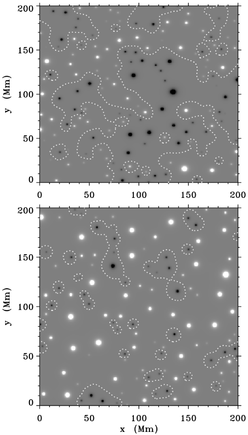
Figure 1.— Simulated photospheric magnetograms for random time steps in a quiet Sun simulation with $\xi=0$ (top) and a coronal hole simulation with $\xi=0.8$ (bottom). Positive polarities are shown as white, negative polarities are shown as black (each saturated at $|B_{z}|=100$ G), and the locations of magnetic neutral lines (where $|B_{z}|=0$) are overplotted as white dotted curves.

Figure 1 shows simulated magnetogram images for representative time snapshots in two of the models: one for a region of balanced magnetic flux ($\xi=0$) and one for a large degree of imbalance ($\xi=0.8$). The continuous magnetic field strength at the photosphere ($z=0$) was calculated using the multiple monopole model described in Section 5.1. A medium gray shade denotes $B_{z}\approx 0$, and the saturation to white and black is imposed at $B_{z}=+100$ and $-100$ G, respectively. For the balanced case, the neutral line meanders through the domain stochastically and splits the region into two roughly equal areas. For the imbalanced case, the neutral lines surround and confine the regions of minority polarity.

The balanced “quiet Sun” model shown in Figure 1(a) has an average total number of flux elements $N=163$, with roughly equal numbers of positive and negative elements and an average absolute flux per element of $8.9\times 10^{18}$ Mx. The imbalanced “coronal hole” model shown in Figure 1(b) has an average total $N=122$, with approximately 81 of the elements being positive and 41 being negative. Note that if the absolute flux per element was equal for the positive and negative populations, we would have expected that $N(1+\xi)/2=110$ elements would be positive, and $N(1-\xi)/2=12$ elements would be negative. Since the number of positive [negative] elements is smaller [larger] than predicted, it is clear that the two populations must have different average absolute fluxes. In fact, for the $\xi=0.8$ model, the average fluxes per element in the positive and negative sets were $2.3\times 10^{19}$ Mx and $5.1\times 10^{18}$ Mx, respectively.

Figure 2.— Time evolution of statistical quantities in the (a) $\xi=0$ and (b) $\xi=0.8$ photospheric models. The temporal variability of the box-averaged absolute flux density $B_{\rm abs}$, the total number $N$ of flux elements in the simulation (divided by 100 to keep the curve in the same plotting domain as the other curves), and the flux imbalance ratio $\xi$ are shown as labeled.

In Figure 2 we plot the time dependence of several statistical quantities for the $\xi=0$ and $\xi=0.8$ cases. These models reached dynamical equilibrium in only about 5 days of simulation time, and only the first 40 days are shown. After a stochastic steady state has been established, the level of continuing temporal variability appears similar in character to the simulations of Parnell (2001) and Crouch et al. (2007). Note that the imbalance ratio $\xi$ does not approach a rigidly constant value, but instead fluctuates with a standard deviation that is typically 2%–10% of its mean value.

Comparing Figures 2(a) and 2(b), we see that as $\xi$ increases the mean of the absolute flux density $\langle B_{\rm abs}\rangle$ increases and its variance decreases. Larger values of $\xi$ correspond to lower rates of flux emergence (see Equation (3)), so that a typical flux element in the large-$\xi$ simulation tends to have a longer lifetime before it is destroyed. However, the functional form of $E(\xi)$ is not the only reason for the increase in $B_{\rm abs}$ with increasing $\xi$. It is possible to illustrate such an increase with a simple analytic model that assumes a constant emergence rate. If the emergence rate $E$ is fixed, but the box-averaged rate of cancellation is assumed to be proportional to the product of the positive and negative flux densities present in the box, then their time evolution can be approximated to be a simple balance between these two effects, with

$$\frac{\partial B_{+}}{\partial t}\,=\,\frac{\partial|B_{-}|}{\partial t}\,=\,E-CB_{+}|B_{-}|\,\,.$$ (9)

In a steady state, the time derivatives can be ignored and we can solve for $E=CB_{+}|B_{-}|$. The individual values of the constants $E$ and $C$ do not need to be specified explicitly, but let us assume their ratio $E/C$ is a known constant called $B_{0}^{2}$. Thus, it becomes possible to solve for the absolute flux density in closed form,

$$B_{\rm abs}\,=\,B_{+}+|B_{-}|\,=\,\frac{2B_{0}}{\sqrt{1-\xi^{2}}}\,\,.$$ (10)

The above expression shows how $B_{\rm abs}$ must increase with an increasing imbalance ratio $\xi$, even in the case where $E$ is independent of $\xi$.

Figure 3 shows how the time-steady values of $\langle B_{\rm abs}\rangle$ from the simulations vary as a function of $\xi$. The error bars on these model points show $\pm 3$ standard deviations around the mean values. To ensure that specific realizations of the random number sequences did not affect the results, the means and standard deviations for each value of $\xi$ were computed from three independent runs of the BONES code. Each run used a different random seed, and each run was performed for a total of 400 days of simulation time. The modeled absolute flux densities generally fall between the observationally expected limiting values of about 3 and 10 Mx cm^-2. Figure 3 also shows two curves that illustrate the functional dependence of the simple analytic estimate of Equation (10) above. The two curves, which were computed using the arbitrary normalization constants $B_{0}=1.4$ and 2.1 G, appear to bracket the modeled points surprisingly well.

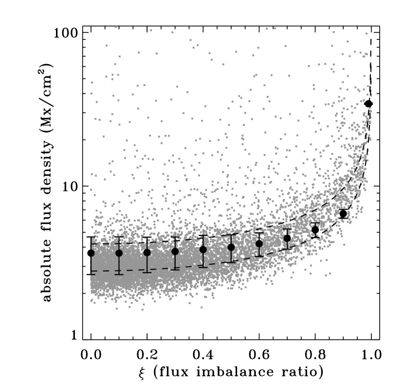
Figure 3.— Steady-state dependence of absolute flux density $B_{\rm abs}$ on the flux imbalance ratio $\xi$. Mean results from the BONES simulations (filled circles, with $\pm 3\sigma$ error bars) are compared with observational data computed from SOLIS full-disk magnetograms (gray points), and with the analytic approximation given by Equation (10) (dashed curves).

In Figure 3 we also plotted measurements made by the Vector SpectroMagnetograph (VSM) instrument of the Synoptic Optical Long-term Investigations of the Sun (SOLIS) facility (Keller et al., 2003). We used publicly available full-disk longitudinal magnetograms taken in the Fe I 6301.5 Å line. Over the time period from August 2003 to November 2009, we obtained one magnetogram per month for a total of 73 individual full-disk maps. For each magnetogram we generated a grid of “macropixels” covering the central part of the solar disk (out to 0.7 $R_{\odot}$ from disk-center). Each macropixel was defined to be $100\times 100$ magnetogram pixels, or 113^′′ square (see also Hagenaar et al., 2008). For each macropixel, we measured the average flux densities of the positive and negative polarities, $B_{+}$ and $B_{-}$, and computed $B_{\rm abs}$ and $\xi$ as defined in Section 3.1. A total of 8264 individual measured data points are shown in Figure 3.

The bulk of the low field-strength SOLIS data shown in Figure 3 appear to follow the same general increasing trend with $\xi$ as do the modeled points and analytic curves. The “long tail” in the data points that extends upward to 10–100 Mx cm^-2 represents times when the macropixels covered parts of active regions. Points on the upper-left of the plot represent active regions that were mostly centered in the macropixel, and points on the upper-right represent times when only one dominant polarity of an active region was in the macropixel. The models presented in this paper are generally meant to be simulations of quiet Sun and coronal hole regions, which are sampled by the majority of weak-field data points in the lower part of Figure 3.

4.2. Number Distributions of Flux Elements

An additional way to verify that the BONES simulations produce magnetic fields similar to those on the real Sun is to examine the probability distributions of element fluxes and compare them with observed distributions. Because the simulations typically have only 100–200 elements in them at any one time, we sampled the distributions a number of times in order to accumulate statistics appropriate for a large number of uncorrelated patches of Sun. In the models, the time cadence for this sampling was fixed at 30 days. This time cadence was found to be more than adequate for the requirement that any given distribution of flux elements must be completely recycled from (i.e., uncorrelated with) the distribution at the previous sampling time. For each case discussed below, the simulations were run until the total number of collected flux elements exceeded $10^{5}$.

Figure 4 shows example distributions for the two models discussed above ($\xi=0$ and 0.8). The distributions of positive and negative polarity elements are plotted separately. For comparison, the analytic distribution of emerging flux elements given by Equation (4) is also shown. This latter distribution has been scaled down in flux by a factor of two (i.e., shifted to the left in the plot) to show the distribution of fluxes in the individual poles of the emerging bipoles, not the total absolute flux in the bipoles as specified by Equation (4). For ease of comparison with observations, these plots are shown in the same general format as Figures 4 and 6 of Parnell (2002) and Figures 2 and 3 of Hagenaar et al. (2008).

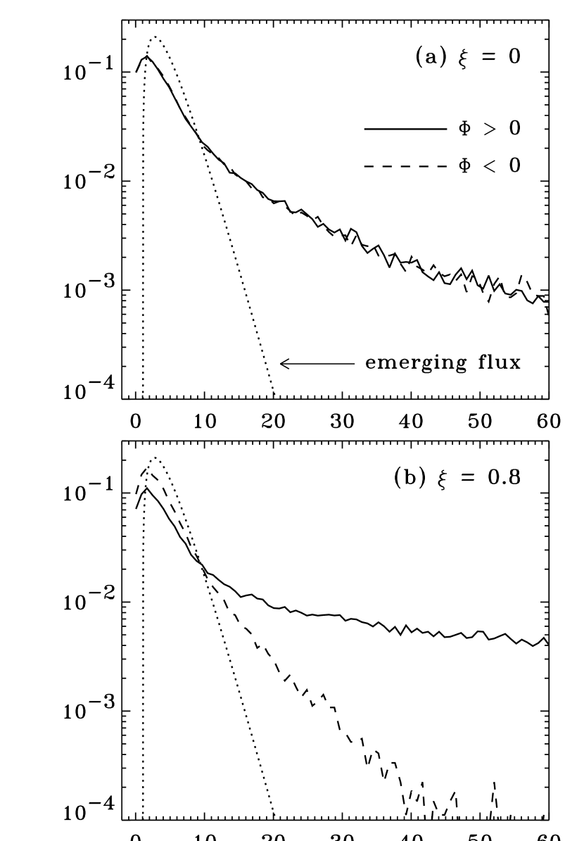
Figure 4.— Statistical number distributions of flux elements as a function of their absolute fluxes in the (a) $\xi=0$ and (b) $\xi=0.8$ models. The time-steady distributions in the numerical simulations are shown separately for positive (solid curves) and negative (dashed curves) polarities, and both are compared with the imposed distribution of emerging flux elements (dotted curves). For plotting convenience, both the fluxes themselves and the normalized probability distributions were divided by $10^{18}$.

The time-steady distributions shown in Figure 4 are substantially “flatter” than the initial distribution of emerging flux elements. In other words, the fluxes have spread out from the relatively narrow range of injected fluxes (roughly $10^{18}$–$10^{19}$ Mx) to both lower and higher values (see Parnell, 2002). Most noticeably, the populations of flux elements with $|\Phi|\gtrsim 3\times 10^{19}$ Mx are hugely enhanced with respect to the distribution of injected flux elements. These stronger flux elements must be the result of mergings between smaller elements of like polarity. In addition, the existence of this enhanced strong-flux tail is the reason that the mean flux per element is larger than the mean flux in a newly emerged flux element (see Section 4.1).

Although it is difficult to see in the plots, there is also a significant number of elements in the simulations with fluxes below the minimum emergent flux per element ($\Phi_{\rm min}/2=10^{18}$ Mx). These weakest flux elements must be the result of fragmentation and partial cancellation. For the $\xi=0$ case, 22% of the flux elements have fluxes less than this threshold value. Because of their small fluxes, however, these account for only about 2.7% of the total absolute flux in the simulation. For the $\xi=0.8$ case, 18% of the flux elements have fluxes below the emerging threshold value, and they account for 1.2% of the total absolute flux.

Figure 4(b) shows the difference between the distributions of positive and negative elements for the imbalanced case of $\xi=0.8$. Overall, the majority polarity has a flatter distribution than does the minority polarity, but there is an excess of minority polarity elements for the weakest fluxes ($|\Phi|\lesssim 10^{19}$ Mx). This is in good agreement with the observational conclusions of Zhang et al. (2006) for coronal holes. Also, the differences in shape shown in Figure 4(b) are highly reminiscent of the flux element distributions shown in Figure 2 of Hagenaar et al. (2008) for coronal holes.

4.3. Naturally Occurring Supergranular Scales

The resemblance between the cellular pattern of solar granulation and that of the larger-scale supergranulation has long been interpreted as evidence that both phenomena are manifestations of the Sun’s convective instability (e.g., Leighton et al., 1962; Roxburgh & Tavakol, 1979; Simon & Weiss, 1991; Rieutord & Rincon, 2010). However, because the flow patterns in the supergranular network are weak and intermittent, it has not been possible to definitively prove their convective origin. It may be that multiple interactions between granule-scale structures produce a distributed network of downflows that in turn seeds horizontal supergranular flows and the aggregation of strong network fields (Rast, 2003; Goldbaum et al., 2009). Alternately, the opposite may be the case; i.e., it may be the aggregation of small-scale magnetic fields that gives rise to the weak supergranular flows (Crouch et al., 2007). In this section we show that the BONES simulations provide some evidence for the initial magnetic-field aggregation described in the latter scenario.

How are the spatial scales of supergranulation measured? It is well known that the dominant cell sizes are of order 10–30 Mm, but different types of measurement give different answers. Simon & Leighton (1964) found cell diameters around 32 Mm by interpreting autocorrelation functions of chromospheric Dopplergrams. Singh & Bappu (1981) traced the cells manually, based on Ca II K-line intensity images, and found diameters of $\sim$22 Mm. Wang (1988) and Wang et al. (1996) applied the autocorrelation technique to magnetograms and found scale sizes between 10 and 25 Mm, depending on the precise diagnostic techniques used. Finally, De Rosa & Toomre (2004) and Hagenaar et al. (1997) used a range of sophisticated algorithms to trace and characterize supergranular boundaries, and found average diameters of only $\sim$15 Mm.

Because the BONES simulations predict only the properties of the magnetic field—and neither the chromospheric emission nor the Doppler velocities—we decided that the most straightforward comparison to make would be with the measured magnetogram autocorrelation functions of Wang (1988). First, a random time step from each of the 11 models was used to create simulated magnetograms similar to those shown in Figure 1. Then, for each $y$ row in the magnetogram, we computed a series of one-dimensional autocorrelation functions in the $x$ direction for the scalar value of $B_{z}$, i.e.,

$$AC(x^{\prime},y)\,=\,\int_{-\infty}^{+\infty}B_{z}(x,y)\,B_{z}(x+x^{\prime},y)\,dx\,\,,$$ (11)

which was then normalized such that $AC(0,y)=1$. Figure 5(a) shows an example autocorrelation function from the $\xi=0$ simulation, plotted as a function of the lag parameter $x^{\prime}$. Similar results were found when the roles of the $x$ and $y$ coordinates were reversed.

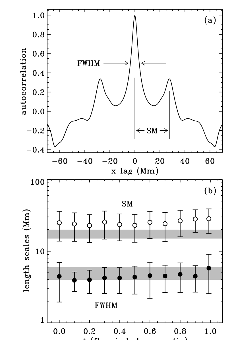
Figure 5.— (a) Example of a simulated magnetogram autocorrelation function for a slice across the $\xi=0$ model, plotted as a function of the lag parameter $x^{\prime}$ (see Equation (11)). (b) Results for modeled mean values of FWHM (filled circles) and SM (open circles) plotted as a function of $\xi$, with error bars denoting $\pm 1\sigma$ in the simulated distributions of values, and the observed ranges of FWHM and SM values from Wang (1988) (gray regions).

We characterized the model autocorrelation functions by finding both the full-width at half-maximum (FWHM) of the central peak and the distance between the central peak and the next secondary maximum (SM). Doing this for each value of $y$ gave rise to ensembles of values for FWHM and SM in each of the 11 simulations. Figure 5(b) shows the mean values for each of these ensembles, along with error bars that show $\pm 1$ standard deviations about the means. There is no significant $\xi$ dependence in the modeled values. For all 11 simulations, the average model FWHM is 4.48 Mm and the average SM distance is 25.1 Mm. These values compare favorably to the solar observations reported by Wang (1988) (shown as gray bars in Figure 5), who found FWHM values between 4 and 6 Mm, and SM distances of 15 to 20 Mm.

The benefit of making a direct comparison between simulated and observed FWHM and SM values is that there is no need to interpret these quantities in terms of arbitrarily defined cell diameters. The models appear to succeed in roughly reproducing the observed autocorrelation properties of the network. It may be possible to explain this success by invoking processes of diffusion-limited aggregation as suggested by Crouch et al. (2007). In this picture, time-steady magnetic structures “collect” on specific scales that depend on the combined emergence, diffusion, and cancellation of flux elements. Supergranular flows may then occur as a result of the magnetic structuring. Crouch et al. (2007) performed tests with a Monte Carlo model that varied several of the discrete step sizes and interaction distances, and found that the resulting supergranular scale size does not depend on these input parameter choices. Instead, it is the overall level of flux emergence and horizontal diffusion—which in turn drives the cancellation rate—that sets the time-steady distance between network concentrations.

5. Coronal Field Evolution

One of the major goals of this paper is to explore how the complex photospheric fields in the magnetic carpet connect with time-variable open flux tubes and closed loops in the extended corona. Thus, here we describe how the field lines are traced upwards and are evolved in time (Section 5.1), we summarize the resulting open and closed fields as a function of the flux imbalance ratio $\xi$ (Section 5.2), we compute relevant time scales for the opening up of closed flux tubes (Section 5.3), we estimate the amount of magnetic energy that emerges in the form of bipoles (Section 5.4), and we compare it to the energy released into the solar wind by magnetic reconnection (Section 5.5).

5.1. Field-line Extrapolation Method

As summarized in Section 2, we compute the vector magnetic field ${\bf{B}}$ above the photospheric surface by assuming the field is derivable from a scalar potential. In other words, each flux element is assumed to act as a monopole-type source, with

$${\bf B}({\bf r})\,=\,\sum_{i}\frac{\Phi_{i}}{2\pi}\frac{{\bf r}-{\bf r}_{i}}{|{\bf r}-{\bf r}_{i}|^{3}}\,\,,$$ (12)

where the coordinates ${\bf r}_{i}=(x_{i},y_{i},z_{i})$ specify the locations of each flux element $i$, and the field point ${\bf r}=(x,y,z)$ can be located anywhere at or above the photosphere ($z\geq 0$). $\Phi_{i}$ is the signed magnetic flux in each element (see, e.g., Wang, 1998; Close et al., 2003).

To avoid singularities at the solar surface, all elements are assumed to be “submerged” below the photosphere (Seehafer, 1986; Longcope, 2005). For simplicity we assumed that all flux elements are at a constant depth. We chose an optimum value of $z_{i}=-1$ Mm on the basis of the following considerations. The peak magnetic field strength $B_{\rm peak}$ in the photosphere, due to a single flux element, occurs right over the point itself at $x=x_{i}$, $y=y_{i}$, and $z=0$. Thus,

$$B_{\rm peak}\,=\,\frac{\Phi_{i}}{2\pi z_{i}^{2}}\,\,.$$ (13)

We want to ensure that $|B_{\rm peak}|$ is less than the equipartition field strength $B_{\rm max}$ for all elements in the simulation (see Section 3.1). Because we do not model pores and sunspots, we can apply this constraint to elements up to a maximum flux of $|\Phi|\approx 10^{20}$ Mx. Thus, applying the condition $|B_{\rm peak}|\leq B_{\rm max}$ to Equation (13) for this value of the flux gives rise to $|z_{i}|\gtrsim 1.1$ Mm. On the other hand, observations have shown that the field strength in a recently emerged ER is at least a few hundred Gauss (Martin, 1988). For the average flux in one pole of an emerging ER (i.e., $\langle\Phi\rangle/2\approx 4.5\times 10^{18}$ Mx), we apply the condition $B_{\rm peak}\gtrsim 100$ G and obtain an upper limit $|z_{i}|\lesssim 0.85$ Mm. The two above constraints on the magnitude of $z_{i}$ are formally incompatible with one another, but the value $\sim$1 Mm appears to be a likely compromise between the two.

The BONES code contains a subroutine that can either trace field lines up from the photospheric surface or down from a larger height. The incremental path length $\Delta s$ for numerical steps taken along the field varies with height, from a minimum value of 0.03 Mm at the photosphere to a maximum value of 10 Mm at a height of $z=200$ Mm. At intermediate heights,

$$\Delta s\,=\,(0.03\,\,\mbox{Mm})^{1-\zeta}(10\,\,\mbox{Mm})^{\zeta}\,\,,$$ (14)

where $\zeta=z/(200\,\,\mbox{Mm})$. Field lines that begin at the photosphere are traced until they either curve back down to intersect the $z=0$ plane again (and are called “closed”) or they climb past a maximum height of 200 Mm (and are called “open”). As discussed in Section 2, on the real Sun it is possible that many flux tubes that reach higher than 200 Mm may eventually be closed back down in the form of large-scale helmet streamers. Whether this occurs or not depends on the global distribution of magnetic flux across the entire solar surface. In any case, it is likely that some plasma that reaches large heights in streamers also interacts with the accelerating solar wind (Wang et al., 2000), so it may not be too erroneous to classify these field lines as open.

When the Monte Carlo simulation of the photospheric field settles into a dynamical steady state (defined here as $t\geq 50$ days), we begin tracing field lines in order to compute the coronal vector field in each time step. This essentially assumes that any temporal changes occur “instantaneously;” i.e., with a time scale shorter than $\Delta t=5$ min. In similar kinds of potential-field simulations, Regnier (2009) found that the actual delay between a given photospheric impulse and the response higher up in the corona is only of order 2 min. Thus, our assumption that ${\bf B}({\bf r})$ can be recomputed from each time step’s new lower boundary condition appears to be reasonable.

In order to quantify the changes that occur in the magnetic field from one time step to the next, we trace a set of field lines that is associated with the $N$ flux elements on the surface. The general idea is to compare the open/closed topology of flux tubes that can be identified unambiguously both at the beginning of a time step and at the end (see also Close et al., 2005). If a flux element moves around on the surface and does not undergo substantial merging, cancellation, or fragmentation, then we can say that it has “survived” that time step, and thus it makes sense to evaluate how its open/closed connectivity may have changed. In cases where the merging, cancellation, or fragmentation makes only a minor change to an original element’s flux, we also consider that element to have survived when the element’s flux changes by less than a specified fractional threshold $\delta$. In most runs of the BONES code presented below, $\delta=0.1$. This means that if a flux element ends the time step with a flux that is within 10% of its original flux, it is classified as being the same element. Flux elements that cannot be tagged in this way are not counted. We discuss the effects of varying the $\delta$ parameter below.

Rather than just trace one field line from each flux element, we instead chose to more finely resolve the coronal magnetic field by tracing seven field lines from each element. The initial footpoints of these seven field lines are arranged in a hexagonal pattern with respect to each flux element’s circular “patch” on the surface. One field line is centered on the flux element. The other six are arranged in a ring around the central point with an angular separation of 60°, each at a horizontal distance of $r_{c}(1+p)/2$ from the central point. This distance is halfway between the flux element’s intrinsic radius $r_{c}$ and its critical interaction distance as defined in Section 3.4. At the beginning of each time step the BONES code traces $7N$ field lines and tags each footpoint with a unique (nonzero) numerical identifier. Each of the flux tubes associated with element $i$ is assigned an equal magnetic flux $\Phi_{i}/7$. During the progress of each time step, new flux elements that emerge are given an identifier of zero. Also, if merging, cancellation, or fragmentation changes the flux in an element to a degree greater than the relative threshold $\delta$, its numerical identifier is reset to zero. At the end of each time step, the coronal field is traced again for the subset of surviving flux elements that have nonzero numerical identifiers. The magnetic flux in those elements is grouped into four bins that are defined by whether the flux tubes were open or closed at the beginning of the time step, and whether they are open or closed at the end. Section 5.2 discusses the distributions of magnetic flux in those four bins.

We note that our method of accounting for the open and closed magnetic flux has several potential shortcomings. By not counting either the newly emerged flux elements or those that undergo substantial merging, cancellation, or fragmentation, we run the risk of not seeing fields that may be releasing lots of energy via magnetic reconnection. We will see below, though, that the magnetic-carpet evolution is not so vigorous that these flux elements represent a significant fraction of the total number. In fact, for most models the fraction of magnetic flux that is missed by not counting these “rapid evolvers” is only of order 5% to 15%. Another possible limitation of our method is that we trace the identities of individual flux tubes for only one time step. If we wanted to measure more accurate time scales for flux reconfiguration, it may have been advantageous to follow field lines for more than just one time step. However, since the magnetic carpet keeps evolving, the number of flux tubes that would become uncountable (i.e., missed by virtue of exceeding the threshold $\delta$) increases for each additional time step over which flux-tube survival would be traced. Following field lines only over the course of one time step, with $\Delta t=5$ min, gave the best balance of time resolution and flux capturing.

5.2. General Results

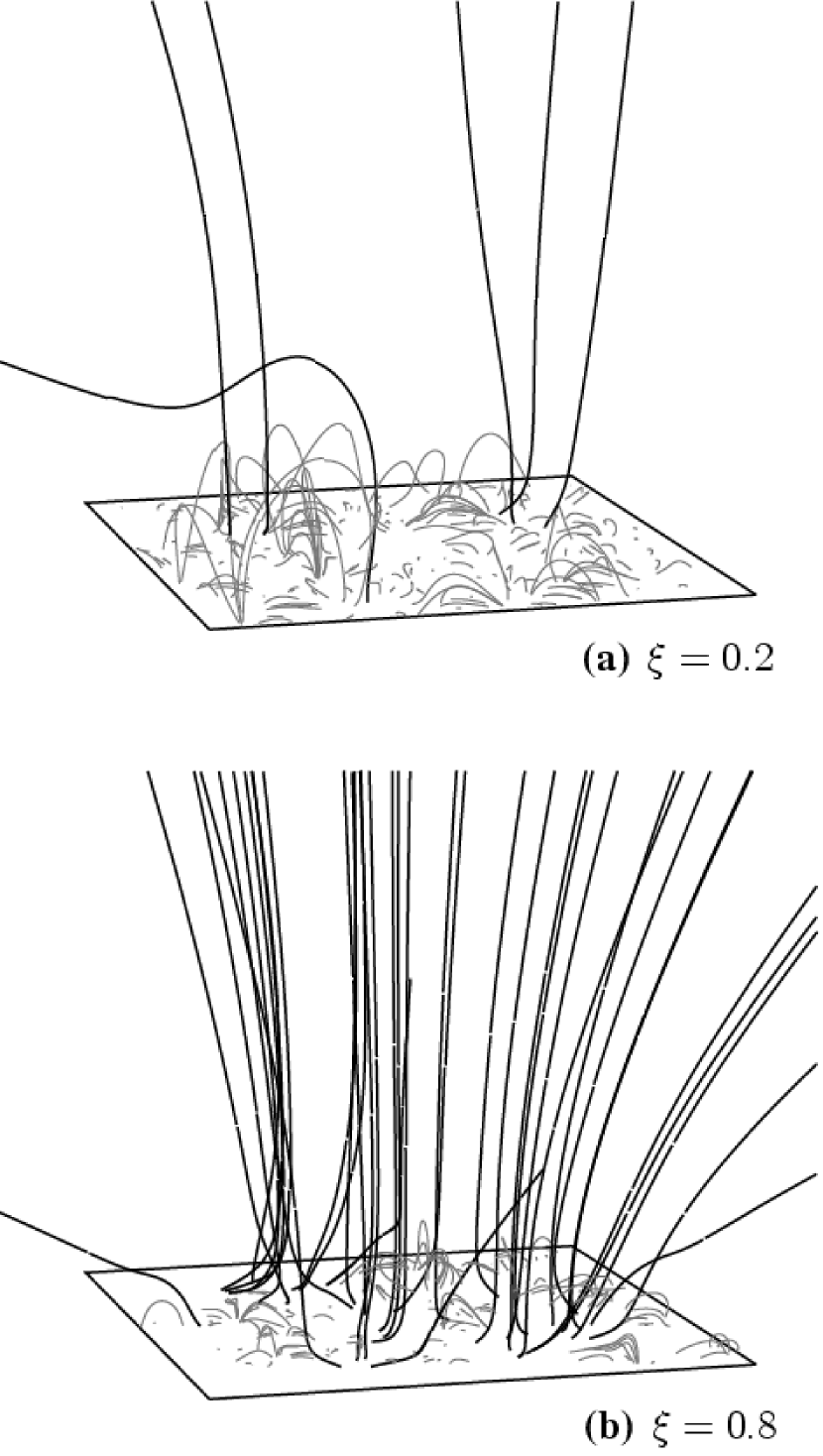
Figure 6.— Traced magnetic field lines at example time steps in BONES models having (a) $\xi=0.2$, and (b) $\xi=0.8$. Open and closed field lines are plotted in black and gray, respectively. In both panels, the horizontal box outlines the (200 Mm)² photospheric simulation domain. The vertical scaling has been stretched by about a factor of two, such that the uppermost tips of the field lines are at a height of $z\approx 110$ Mm.

Figure 6 illustrates a selection of field lines for BONES models with a mostly balanced lower boundary ($\xi=0.2$) and a highly imbalanced lower boundary ($\xi=0.8$). The three-dimensional field lines are shown projected into a two-dimensional plane that is defined by an observer viewing the scene at an inclination angle 82° from the normal to the photosphere. Two different shades denote closed versus open field lines. Models with more imbalanced fields (i.e., higher values of $\xi$) have both a larger fraction of open flux and a smaller vertical extent for the closed loops. Both of these trends are examined quantitatively below.

We studied the statistical properties of the closed loops in the simulations by tracing large numbers of field lines from random starting locations $(x,y,0)$ in the photosphere. Example time snapshots from the 11 models (with varying $\xi$ values) were used to trace at least 5000 loops in each model. For the six models with $\xi\leq 0.5$, for which there were fewer open field lines, we were able to compute at least 20000 loops. The maximum heights of these loops were collected into 11 statistical distributions, one for each model. Although the means and standard deviations of these distributions were computed, the distributions were far from Gaussian in shape. Thus, we quantified them further by computing percentile intervals $H_{n}$ of the sorted cumulative distributions of heights. For example, 25% of the loops have heights less than the quartile height of $H_{25}$, and 50% of the loops have heights less than the median height of $H_{50}$. We also computed $H_{75}$ and $H_{95}$, with the latter being an approximate indicator of the largest loops (without being dependent on the statistically insignificant tail of the very largest loops).

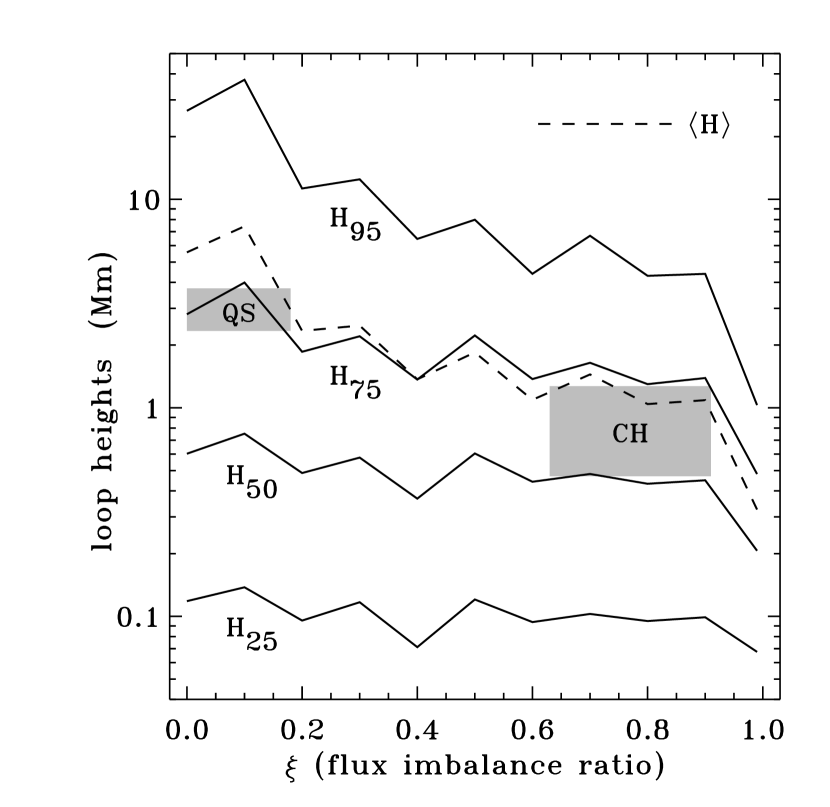
Figure 7.— Variation of percentile intervals of the sorted statistical distributions of loop heights, shown as a function of $\xi$. Percentiles at the 25%, 50%, 75%, and 95% levels (solid curves) are compared with the mean loop height $\langle H\rangle$ (dashed curve) and with observationally inferred values from Wiegelmann & Solanki (2004) for quiet Sun (QS) and coronal hole (CH) regions (gray boxes).

Figure 7 shows how the percentile intervals vary as a function of the flux imbalance ratio $\xi$. On the smallest spatial scales (i.e., for granule-sized loops characterized by $H_{25}$ and $H_{50}$) there does not appear to be a significant dependence on $\xi$. However, the longest loops follow the trend that is visually apparent in Figure 6; i.e., the more balanced the photospheric field, the larger the loops. This trend is apparent not only in $H_{75}$ and $H_{95}$, but also in the mean height $\langle H\rangle$ that is weighted more strongly by the longest loops.

Figure 7 also shows approximate observational ranges of mean loop heights for quiet Sun (QS) and coronal hole (CH) regions as determined by Wiegelmann & Solanki (2004). These loop-height calculations were similar to ours in that they were based on potential-field extrapolations from photospheric lower boundary conditions, but Wiegelmann & Solanki (2004) used observed magnetograms from the Michelson Doppler Imager (MDI) instrument on SOHO (see also Close et al., 2003; Tian et al., 2010; Ito et al., 2008). The overall agreement with the modeled $\xi$ dependence of $\langle H\rangle$ is good. The general trend for high-$\xi$ CH regions to have shorter loops than low-$\xi$ QS regions is also consistent with the trend pointed out by Feldman et al. (1999) and Gloeckler et al. (2003) for the source regions of fast solar wind to be correlated with short loops and the source regions of slow wind to be correlated with long loops.

A representative illustration of the footpoints of open field lines is given in Figure 8 for the $\xi=0.8$ model. This plot shows the locations of the photospheric footpoints of $10^{4}$ field lines that were traced down from an evenly spaced grid at the top ($z=200$ Mm). In order to account for the horizontal flaring of potential field lines from the finite-sized simulation box, the grid of $100\times 100$ starting points had an overall horizontal size of $1800\times 1800$ Mm in the $x$ and $y$ directions (centered on the $200\times 200$ Mm simulation box). The overall appearance of Figure 8 is highly reminiscent of the observed supergranular network. The apparent “cell diameters” tend to be between 20 and 40 Mm as on the real Sun. Note also the appearance of thin channels, stretched between smaller knots of closed-field regions, that appear to support the connectivity theorems described by Antiochos et al. (2007).

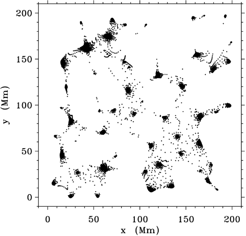
Figure 8.— Photospheric locations of footpoints of “open” magnetic field lines traced down from an evenly spaced grid at a height of $z=200$ Mm, for one time snapshot of the $\xi=0.8$ model.

All of the $10^{4}$ open field lines with footpoints shown in Figure 8 are of positive polarity. This is the dominant polarity as specified by the initial conditions of the BONES code (see Section 3.1). All negative polarities end up connected to positive polarities in closed loops, and thus there are no “open funnels” with the non-dominant polarity. Of course, this is also a highly simplified situation when compared to the real Sun, for which there are often network concentrations of both polarities even in strongly unipolar coronal holes.

As described above, at the beginning of each time step there is a set of field lines traced from each of the flux elements. These $7N$ field lines are used to estimate the instantaneous fractions of absolute unsigned flux that are either open or closed. The fraction of flux that is open is denoted $f_{\rm open}$, and in Figure 9 we show its mean value as a function of the $\xi$ imbalance ratio. This fraction is never exactly the same from one time step to the next, and the error bars show $\pm 1$ standard deviations about the mean values. On average, $f_{\rm open}$ is roughly equal to $\xi$ itself. In other words, models with balanced fields tend not to have much open flux, but when there is an increase in the unbalanced component of the field there is a corresponding increase in the fraction of open flux. Figure 9 also compares the modeled values of $f_{\rm open}$ with observational determinations of this quantity from Wiegelmann & Solanki (2004), and there is a similar trend of direct proportionality, with $f_{\rm open}\approx\xi$.

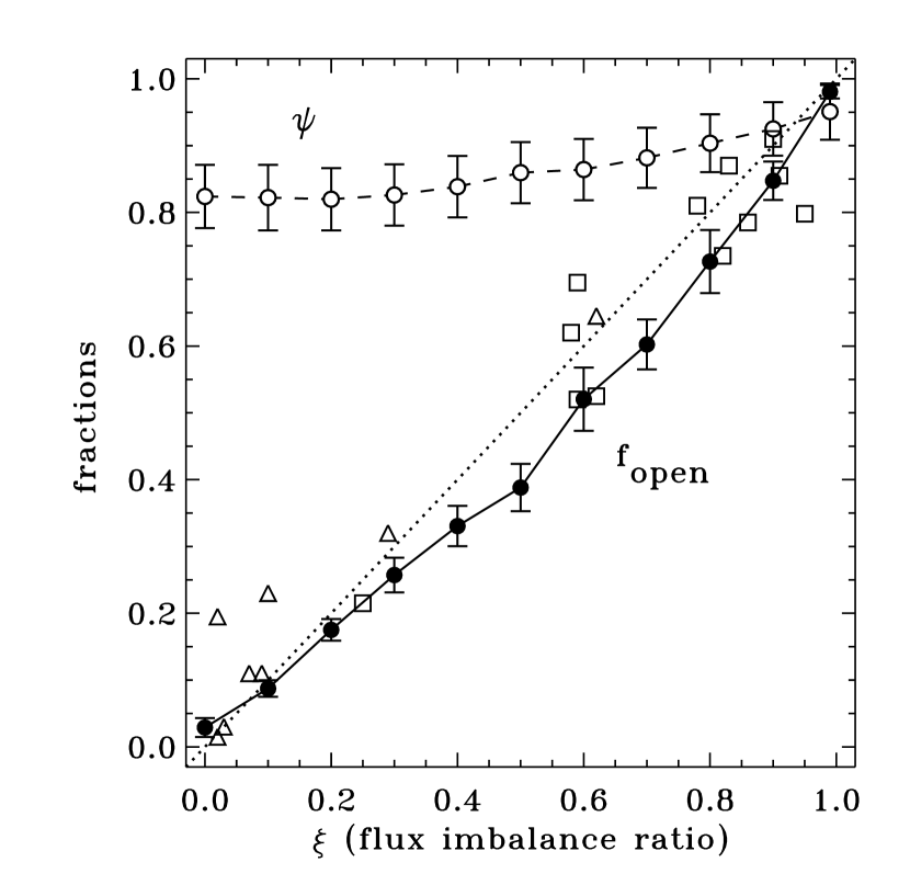
Figure 9.— Various dimensionless flux fractions shown as a function of $\xi$: mean values of $f_{\rm open}$ (filled circles) and mean values of $\psi$ (open circles), both with their $\pm 1\sigma$ spreads shown as error bars, and observational estimates of $f_{\rm open}$ from Wiegelmann & Solanki (2004) in QS (triangles) and CH (squares) regions.

5.3. Comparison of Relevant Time Scales

We studied the time evolution of magnetic topology in the BONES simulations by following the opening and closing of flux tubes from the beginning to the end of each time step. For comparison, we also computed the recycling time scale for flux to emerge from below the photospheric surface (see also Section 3.2). We defined this quantity as

$$\tau_{\rm em}\,=\,\frac{\langle B_{\rm abs}\rangle}{E}\,\,.$$ (15)

For our models we took $\langle B_{\rm abs}\rangle$ from Figure 3 and $E$ from Equation (3), and we found that the emergence time scale $\tau_{\rm em}$ tends to have values around 1–2 hr (see Hagenaar et al., 2008). Regions of extreme flux imbalance undergo slower emergence, with $\tau_{\rm em}$ exceeding 10–20 hr when $\xi\gtrsim 0.9$. Figure 10(a) shows the $\xi$ dependence of this time scale.

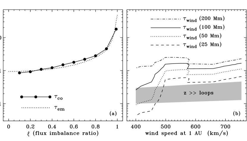
Figure 10.— Comparison of time scales for various models. (a) For the Monte Carlo models of the magnetic carpet, the recycling time for flux emergence (dotted curve) is compared with the time scale for flux opening (filled circles and solid curve). (b) For the Cranmer et al. (2007) solar wind models, we plot acceleration times $\tau_{\rm wind}$ up to heights of 25 Mm (dashed curve), 50 Mm (dotted curve), 100 Mm (solid curve), and 200 Mm (dot-dashed curve) versus the outflow speeds at 1 AU. Also shown is an approximate region of parameter space that corresponds to upper heights $z$ that exceed 2–3 times the maximum heights of closed loops in the corresponding BONES models (gray box).

Next we used the flux tubes traced in our simulations to investigate the time scales for magnetic field evolution in the corona. Close et al. (2005) performed a similar study in the limit of a balanced field, with $\xi=0$. They computed a so-called coronal flux recycling time that is meant to characterize a local rate of change of the coronal field. This rate is driven both by reconnection and by topological evolution of the complex “hierarchical tree” of footpoint domains in the magnetic carpet. Because changes in the coronal field can take place even without any flux emergence or cancellation, Close et al. (2005) found that coronal flux recycling times can be significantly shorter than photospheric flux recycling times. Changes in topological connections can occur purely as a result of the horizontal motions of flux elements (e.g., Edmondson et al., 2009, 2010a). Close et al. (2005) used an older photospheric flux recycling time of $\tau_{\rm em}\approx 15$ hr, but they found that the coronal flux recycling time can be as short as 1.4 hr. When emergence and cancellation were suppressed, the coronal time scale was approximately a factor of two larger ($\sim$3 hr) but still much more rapid than $\tau_{\rm em}$. Our models differ from those of Close et al. (2005) in that our photospheric emergence time scale is now of the same order of magnitude as their coronal recycling time scale.

Below we describe how we estimate how long it takes for just the open flux to recycle itself in the corona. We do not track the (possibly more numerous) changes in topology that do not involve open flux tubes. As summarized in Section 5.1, over the course of a time step some of the flux in the model is unaccounted for because it has either emerged since the last time step or it has evolved beyond recognition as the same flux element. The remaining fraction of total absolute flux—i.e., that which survives the time step unaltered—is called $\psi$, and Figure 9 shows how its mean value increases steadily from about 0.82 to 0.95 as $\xi$ increases from 0 to 1. A larger choice for the relative tolerance parameter $\delta$ would give a larger survival fraction $\psi$ (see below), but it can be argued that too much tolerance would give rise to errors in how flux tubes are identified and tracked.

For flux tubes that survive a time step relatively unchanged, we compared the endpoints of the field lines traced at the beginning and end of the time step. The fluxes in these field lines are summed into four separate bins that are defined by their connectivity. The four bins correspond to four fractions of the total surviving absolute flux: $f_{\rm oo}$ (starts open, ends open), $f_{\rm oc}$ (starts open, ends closed), $f_{\rm co}$ (starts closed, ends open), and $f_{\rm cc}$ (starts closed, ends closed). Because the overall magnetic configuration of the system does not vary strongly over a single time step, we found that $f_{\rm oo}\approx f_{\rm open}$. Also, the two fractions that denote change ($f_{\rm oc}$ and $f_{\rm co}$) both tend to be small contributors to the total. The mean values of $f_{\rm co}$ in the models tend to vary between about 0.005 and 0.025, with the largest values occurring for intermediate imbalance ratios of $\xi\approx 0.5$ and the smallest values occurring at the extremes of $\xi=0$ and 0.99. We also note that the time averages of $f_{\rm co}$ and $f_{\rm oc}$ are always roughly equal to one another (as should be required for a time-steady dynamical equilibrium). For all 11 models, the time averages of these two fractions never differ from one another by more than about 2%.

At any one time, we define the amount of open (absolute) flux density as $B_{\rm open}=f_{\rm open}B_{\rm abs}$. We computed the instantaneous rate of opening in each time step $\Delta t$ as

$$\left(\frac{dB}{dt}\right)_{\rm co}\,=\,\frac{f_{\rm co}B_{\rm abs}}{\Delta t}\,\,.$$ (16)

Note that the above definition makes the implicit assumption that $f_{\rm co}$ is the fraction of the total absolute flux density in the simulation that opens up in one time step. However, this fraction is only approximately $\psi$ times the total absolute flux that opens up. We assumed that the small fraction $(1-\psi)$ that was not counted contributes in the same way as the larger fraction $\psi$ that was counted. (This assumption is tested below.) Thus, the mean time scale for the opening up of closed flux tubes is

$$\tau_{\rm co}\,=\,\frac{\langle B_{\rm open}\rangle}{\langle(dB/dt)_{\rm co}\rangle}\,=\,\frac{\langle f_{\rm open}\rangle\,\Delta t}{\langle f_{\rm co}\rangle}\,\,.$$ (17)

Because the quantities $f_{\rm co}$ and $(dB/dt)_{\rm co}$ can be quite variable from time step to time step, we realized that care should be taken in computing the averages in Equation (17). We ended up computing these averages in two independent ways. First, we took simple arithmetic averages of the time series for $(dB/dt)_{\rm co}$ and the other quantities. Second, we integrated the rate defined in Equation (16) as a function of time to build up the cumulative amount of flux density that is opened up over the course of the simulation. This is a monotonically increasing function, but its increase with time is intermittent because different amounts of flux are opened up in each time step. We fit the cumulative growth of opened flux density with a linear function, and then used the slope of this linear fit as the mean value of $(dB/dt)_{\rm co}$. These two methods gave results that agreed with one another to within about 10%, and we used the latter technique for all values reported below.

Figure 10(a) compares the above time scales with one another. It is clear that $\tau_{\rm co}\approx\tau_{\rm em}$ in these models. In other words, the time scale for the replacement of the photospheric flux—via emergence from below—is the same as the time scale for replacement of the open flux that feeds the solar wind. At first glance, this appears to be a simple requirement for a time-steady equilibrium, in the same way that $f_{\rm co}\approx f_{\rm oc}$ is required to maintain a steady state. However, one can imagine situations where the rate of flux evolution in the corona is not so strongly coupled to the emergence rate of new flux from below (e.g., Close et al., 2005). In our case, it is the use of potential fields—which are remapped during each time step with no allowance for the storage of free energy in the corona—that demands $\tau_{\rm co}\approx\tau_{\rm em}$. In other words, the BONES models reproduce the case of highly efficient magnetic reconnection, where the corona “processes” the flux as quickly as it is driven (stressed or injected) from below. One can imagine that in a full MHD simulation the efficiency of magnetic reconnection may not be so high, and thus the resulting non-potential, current-filled corona should exhibit $\tau_{\rm co}>\tau_{\rm em}$.

Note that Figure 10(a) does not show the value of $\tau_{\rm co}$ for the $\xi=0$ model. As Equation (17) makes clear, in this case both the numerator and denominator are numbers that should approach zero. Ideally, there should be no open fields at all in a perfectly balanced potential field. The BONES models do in fact give slightly nonzero values for $\langle f_{\rm open}\rangle$ and $\langle f_{\rm co}\rangle$, but these are believed to be numerical artifacts arising from the discrete nature of the field-line tracing technique. We reiterate that we do not compute the time scale for all of the coronal flux to be recycled. That recycling time should be nonzero even for the balanced $\xi=0$ model (Close et al., 2005). In all models with $\xi\ll 0$, the full coronal recycling time is likely to be significantly shorter than $\tau_{\rm co}$.

In order to study the dependence of our results on the assumptions made about flux-tube identification, we varied the threshold flux identification parameter $\delta$ away from its default value of 0.1, in a range between 0 and 0.5. This parameter sets the relative tolerance for the classification of evolving flux elements over a time step. Table 1 shows several resulting parameters of the test simulations, which were all performed for $\xi=0.4$. As we expected, the flux survival fraction $\psi$ increases monotonically with increasing $\delta$. However, there does not seem to be any definitive trend with $\delta$ in the fraction of flux that opens up ($f_{\rm co}$), the related time scale for flux opening ($\tau_{\rm co}$), or the energy flux released by reconnection into open-field regions ($\langle F_{\rm co}\rangle$, see Section 5.5). This suggests that the topological changes resulting from flux-tube opening are adequately resolved in the simulations. Thus, we retain the standard value $\delta=0.1$ for the remainder of the paper.

Table 1Variation of Mean Magnetic Properties ($\xi=0.4$ model) with $\delta$

$\delta$	$\psi$	$\langle f_{\rm co}\rangle$	$\tau_{\rm co}$	$\langle F_{\rm co}\rangle$
			(hr)	(erg cm-2 s-1)
0.00	0.759	0.0199	1.403	$1.50\times 10^{4}$
0.10	0.839	0.0220	1.222	$1.77\times 10^{4}$
0.25	0.901	0.0219	1.273	$1.65\times 10^{4}$
0.38	0.926	0.0245	1.160	$1.80\times 10^{4}$
0.50	0.938	0.0226	1.233	$1.70\times 10^{4}$

It is worthwhile to compare the time scale for flux opening to the time scale for solar wind acceleration along the open flux tubes. If a significant amount of solar wind plasma flows out during the time it takes the open field to reorganize itself via reconnection, then the reconnection processes themselves probably are not responsible for producing the majority of the solar wind. The RLO idea depends on the plasma in open flux tubes coming from the opening up of closed loops. Thus, we want to determine whether or not a large amount of mass accelerates out in the open flux tubes over the time it would take for significant mass to be processed via loop-opening.

The time scale for wind acceleration from a lower height $z_{\rm TR}$ in the solar transition region (TR) to an arbitrary upper height $z$ is

$$\tau_{\rm wind}(z)\,=\,\int_{z_{\rm TR}}^{z}\frac{dz^{\prime}}{u(z^{\prime})}\,\,,$$ (18)

where $u(z)$ is the radial wind speed. The TR was chosen as the height to start the integration because that is where the mass flux of the wind is thought to be determined (see, e.g., Hammer, 1982; Withbroe, 1988; Hansteen & Leer, 1995). We used the one-fluid solar wind models of Cranmer et al. (2007) to compute $\tau_{\rm wind}$, and we defined $z_{\rm TR}$ as the height at which the temperature in a wind model first reaches $10^{5}$ K.

Figure 10(b) shows the wind acceleration time scales for several representative upper heights $z$, and for a range of models of the fast and slow wind that have speeds at 1 AU between 400 and 750 km s^-1 (see Cranmer et al., 2007). Two side-by-side plots are necessary in Figure 10 because there is not a unique one-to-one correspondence between the flux imbalance ratio $\xi$ and the wind speed at 1 AU. We do know, however, that there is some association between slow wind streams and QS regions on the surface ($\xi\approx 0$) and between fast wind streams and CH regions on the surface ($\xi\approx 1$). Thus, the overall left-to-right variations in the two panels can be roughly associated with one another.

The slow solar wind models shown in Figure 10(b) have the shortest acceleration time scales. Given Equation (18), this is potentially counterintuitive. However, we note that the slow wind models from Cranmer et al. (2007) often have local maxima in $u(z)$ of order 100 km s^-1 in the low corona that are not present in the more steadily accelerating fast wind models (see also Figure 7a of Cranmer, 2010). These regions correspond to enhanced magnetic fields that were included to simulate open fields at the edges of streamers and active regions. Observations are beginning to show hints of such rapid outflows as well (Harra et al., 2008; Subramanian et al., 2010; Bryans et al., 2010).

When comparing the time scales for flux opening and solar wind acceleration, we can use the loop heights illustrated in Figure 7 as an order-of-magnitude guide for the maximum height $z$ to use when computing $\tau_{\rm wind}(z)$. For example, when parcels of solar wind exceed a height that is 2–3 times $H_{95}$, it can be safely assumed that the wind has left behind virtually all interactions with closed loops and should be considered to be freely accelerating. This allows us to compare the time scales between panels in Figure 10 for the two general types of solar wind:

1. For slow wind streams rooted in balanced QS regions (i.e., $\xi\approx 0$), the height at which the wind flows “free and clear” of loops is of order 50–100 Mm. Figure 10(b) shows that this height corresponds to $\tau_{\rm wind}\approx 0.1$–0.3 hr. This is a shorter time scale than the representative flux-opening time $\tau_{\rm co}\approx 1$ hr that corresponds to the left side of Figure 10(a), but it is still of the same order of magnitude. Thus, it is possible that RLO processes could be important for slow wind acceleration.

2. For fast wind streams rooted in unbalanced CH regions (i.e., $\xi\approx 1$), the height corresponding to 2–3 times $H_{95}$ is only of order 5–15 Mm. The fast wind accelerates to this range of heights in less than about 0.3 hr, but the flux-opening recycling time in coronal holes can be as long as 3–10 hr. This is a larger discrepancy than in the case of the slow wind, and it implies that it is unlikely that RLO processes are important in accelerating the bulk of the fast wind. (Of course, it still may be the case that RLO processes produce a highly intermittent or episodic injection of mass and energy into the fast wind in coronal holes—just not enough to affect the majority of the accelerating plasma. The polar jets discussed further in Section 6 may be a prime example of this intermittency.)

The gray box in Figure 10(b) shows the approximate range of wind acceleration time scales that correspond to maximum heights $z$ exceeding about 2–3 times $H_{95}$ as discussed above. The shape of the gray region is roughly independent of wind speed and $\xi$. This is because, as one goes from left to right in the plot, the increase in $\tau_{\rm wind}$ (for constant $z$) is offset by the fact that the relevant value of $z$ decreases (because $H_{95}$ decreases; see Figure 7).

Finally, we reiterate that the values of $\tau_{\rm co}$ shown in Figure 10(a) are likely to just be lower limits to the actual time scales of flux-opening. As discussed above, our models assume a succession of potential fields that are consistent with the assumption of rapid magnetic reconnection. If the true MHD state of the corona exhibits less efficient magnetic reconnection, then the photospheric footpoint stressing will build up non-potential fields and current sheets in the corona and thus give rise to larger net values of $\tau_{\rm co}$. In this case, it is even more certain that $\tau_{\rm co}\gg\tau_{\rm wind}$, and our conclusion that RLO processes are unimportant in accelerating the solar wind is strengthened.

5.4. Poynting Flux in Emerging Bipoles

Our primary reason for constructing the BONES simulations was to estimate how much energy is deposited into the solar wind by the evolving magnetic carpet. First, though, it is necessary to compute how much magnetic energy is being injected into the system from below the photosphere. It is not obvious that all (or even most) of this energy is able to be converted into forms that supply heat or momentum to the accelerating solar wind. Since, on small scales, much of the injected magnetic energy is in the form of compact bipoles, it may be difficult for much of this energy to become “liberated” into the open-field regions when these bipoles evolve and interact with one another. Thus, in this section we discuss the total magnetic energy that is potentially available, and in the following section we estimate what fraction of it is actually released by reconnection into the open-field regions.

The relevant quantity to compute when considering the rate of injection of magnetic energy from below the photosphere is the Poynting flux, which is defined as

$${\bf S}\,=\,\frac{c}{4\pi}{\bf E}\times{\bf B}\,\approx\,-\frac{1}{4\pi}\left[\left({\bf v}\times{\bf B}\right)\times{\bf B}\right]\,\,,$$ (19)

and where the latter approximation assumes the ideal condition of MHD flux freezing. In the Cartesian system studied in this paper, the most relevant component of the Poynting flux is the $z$ component, with

$$S_{z}\,=\,\frac{1}{4\pi}\left[B_{\perp}^{2}v_{z}-({\bf v}_{\perp}\cdot{\bf B}_{\perp})B_{z}\right]$$ (20)

where ${\bf B}_{\perp}$ and ${\bf v}_{\perp}$ are the components of the magnetic field and velocity in the horizontal ($x$–$y$) plane. The two terms on the right-hand side of Equation (20) represent components associated with flux emergence and surface flows, respectively. For simplicity, though, in the remainder of this section we will endeavor only to estimate the overall magnitude $S$ of the Poynting flux. This gives a reliable upper limit that is independent of the adopted geometry and topology of the emerging flux elements.

Observationally, the Poynting flux can be estimated from various measured proxies (e.g., Welsch et al., 2009), but there exist ambiguities in the data that give rise to significant uncertainties. Fisk et al. (1999) estimated the magnitude of ${\bf S}$ to be about $5\times 10^{5}$ erg cm^-2 s^-1 in source regions of the solar wind. Martínez González et al. (2010) used vector magnetic fields measured by Hinode/SOT to estimate that small-scale emerging loops provide something like $10^{6}$ to $2\times 10^{7}$ erg cm^-2 s^-1 to the low chromosphere in quiet regions.

We estimated the magnitude of the Poynting flux for the Monte Carlo models developed above in two independent ways. Figure 11(a) shows that the two methods gave rise to similar ranges of Poynting flux (both of order $10^{6}$ erg cm^-2 s^-1) with a relatively weak dependence on $\xi$. These two methods are described below.

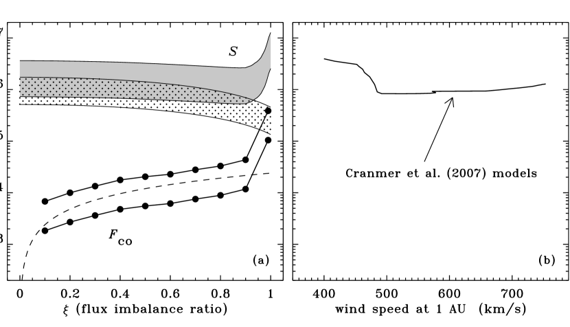
Figure 11.— Comparison of energy fluxes for various models. (a) Estimated flux $\langle F_{\rm co}\rangle$ in loop-opening events (filled circles and solid curves) computed with two choices for $\theta_{\rm L}C_{\rm L}$. Also shown are approximate Poynting fluxes $S$ for photospheric flux emergence, with the dotted region showing estimates from Equation (23) and the gray region showing estimates from Equation (26). The dashed curve shows a linear scaling $\langle F_{\rm co}\rangle\propto\xi$. (b) Total dissipated solar wind energy flux $F_{\rm wind}$ from the WTD models of Cranmer et al. (2007).

First, we note that the emergence rate $E$ (Equation (3)) already describes how much magnetic flux is driven up from below the photosphere, per unit area and per unit time (i.e., its units are Mx cm^-2 s^-1). What we want to know is how much magnetic energy emerges, in units of erg cm^-2 s^-1. Thus, if we can relate the flux in an emerging bipole to its magnetic energy, we can convert easily from $E$ to $S$. Treating a pair of equal-and-opposite emerging flux elements as an an ideal (but partially submerged) magnetic dipole, we can specify its field strength as

$$B\,=\,\frac{\Phi_{i}D}{2\pi r^{3}}\sqrt{1+3\cos^{2}\theta}\,\,,$$ (21)

where $\Phi_{i}$ is the absolute flux in each pole, $D$ is the horizontal separation between the two poles, $r$ is the distance measured from the center of the dipole, and $\theta$ is the polar angle measured from the (horizontal) dipole axis. Assuming the dipole is submerged at a depth $|z_{i}|$, it is possible to integrate the magnetic energy $U_{\rm mag}$ over the full coronal volume $V$ (i.e., over all $x$ and $y$, and all $z>0$) analytically. We thus found

$$U_{\rm mag}\,=\,\int dV\,\frac{B^{2}}{8\pi}\,=\,\frac{\Phi_{i}^{2}D^{2}}{128\pi^{2}|z_{i}|^{3}}\,\,.$$ (22)

Note that the magnetic energy above the photosphere is extremely sensitive to the submerged depth $|z_{i}|$. Once the magnetic energy due to a given bipole is known, we can estimate the magnitude of the Poynting flux as

$$S\,\approx\,E\,\frac{\langle U_{\rm mag}\rangle}{\langle\Phi\rangle}$$ (23)

where the angle brackets denote the properties of the “average” emerging bipole as discussed in Section 3.2. Figure 11(a) shows this quantity for the 11 models as a function of $\xi$, and for two reasonable choices of $|z_{i}|$ (0.8 and 1.2 Mm). For typical values of $E=10^{-3}$ Mx cm^-2 s^-1, $\langle\Phi\rangle=9\times 10^{18}$ Mx, $D=6.8$ Mm, and $|z_{i}|=1$ Mm, we find that $S\approx 8\times 10^{5}$ erg cm^-2 s^-1.

The second way to estimate $S$ was proposed by Fisk et al. (1999). Here, we compute the total magnetic energy in the system (per unit surface area) and divide it by the flux recycling time. In other words,

$$S\,\approx\,\frac{1}{\tau_{\rm em}}\int dz\,\frac{B^{2}}{8\pi}\,\,.$$ (24)

Here, the value of $B$ at the photospheric surface is essentially the time-averaged absolute flux density (i.e., $B_{\odot}\approx\langle B_{\rm abs}\rangle$). It is the height-dependence of $B$, for $z>0$, that is the major source of uncertainty in evaluating Equation (24). However, it is straightforward to follow Fisk et al. (1999) and assume a vertical falloff that depends on a power of heliocentric radius. Thus,

$$B\,\approx\,B_{\odot}\left(\frac{R_{\odot}}{r}\right)^{n}$$ (25)

(where $r=z+R_{\odot}$), and then

$$S\,\approx\,\frac{B_{\odot}^{2}R_{\odot}}{8\pi\tau_{\rm em}(2n-1)}\,\,.$$ (26)

At large distances above the photosphere, the exponent $n$ approaches a value of 2, but it is believed to take on larger values closer to the surface (see, e.g., Banaszkiewicz et al., 1998). For a typical value of $B_{\odot}=4$ G and $\tau_{\rm em}=1$ hr, we can estimate an upper limit on $S$ by assuming $n=2$, and thus obtain $S=4\times 10^{6}$ erg cm^-2 s^-1. For a more realistic coronal value of $n\approx 8$, we have $S\approx 6\times 10^{5}$ erg cm^-2 s^-1. Figure 11(a) shows how $S$ varies as a function of $\xi$ when the modeled variations in $\langle B_{\rm abs}\rangle$ and $\tau_{\rm em}$ are used, and when the two above values of $n=2$ and 8 are assumed to define the lower and upper limiting cases. Given the uncertainties, the two alternate methods of estimating $S$ give numerical values that are quite consistent with one another.

5.5. Energy Release in Loop-Opening Events

We used the output of the BONES simulations to estimate the amount of energy released by magnetic reconnection for cases of closed flux tubes turning into open flux tubes (and vice versa). It is important to note that there are also expected to be many other sites of reconnection and energy release that do not involve open flux tubes. For example, in a balanced QS region there may be a large number of small-scale “footpoint-swapping” events that start with a configuration of closed loops and end with a slightly different topological distribution of closed loops (Priest et al., 2002; Close et al., 2005). In this paper, we explicitly ignore the energy release in the closed–closed events in order to focus on only the subset of events that can input mass and energy into the solar wind.

The basic geometrical picture for a flux-opening event is the “anemone” type structure that is believed to exist at the footpoints of many X-ray bright points, coronal jets, and polar plumes (e.g., Syrovatskii, 1982; Shibata et al., 1992, 2007; Filippov et al., 2009; Shimojo & Tsuneta, 2009). In this picture, a small bipolar magnetic field either emerges or advects into the presence of a larger-scale open field. Magnetic reconnection is believed to occur roughly above the end of the bipole with the opposite polarity as the open field (Edmondson et al., 2009, 2010a). The newly opened flux may take the form of a jet or plume (Wang, 1998), and the newly closed flux may “subduct” and provide heating to the underlying chromosphere (Guglielmino et al., 2008). In one of these interchange-reconnection type events, the amount of closed magnetic flux that opens up should be the same as the amount of pre-existing open flux that becomes closed (i.e., $f_{\rm co}\approx f_{\rm oc}$).

Because we model the evolution of the coronal magnetic field as a succession of potential fields (see Section 2), we use the quasi-static “minimum current corona” (MCC) model to estimate the energy loss due to reconnection (Longcope, 1996; Longcope & Kankelborg, 1999; Beveridge & Longcope, 2006). In this model, the mean energy flux released in closed-to-open reconnection events is proportional to the rate $(dB/dt)_{\rm co}$ at which magnetic flux is opened up (see Equation (16)). For our simulations, we derived the MCC energy flux to be

$$F_{\rm co}\,=\,\theta_{\rm L}C_{\rm L}\frac{\Phi_{1}}{\langle d\rangle}\left|\frac{dB}{dt}\right|_{\rm co}\,\,,$$ (27)

where $\Phi_{1}$ is the mean absolute flux per element, $\langle d\rangle$ is the mean separation between elements in the simulation, and $\theta_{\rm L}$ and $C_{\rm L}$ are dimensionless constants. The Appendix presents a detailed derivation of Equation (27) for anemone-type reconnection events, including a discussion of the most likely numerical values for $\theta_{\rm L}$ and $C_{\rm L}$.

It is important to clarify that the energy flux given by Equation (27) is meant to be an order-of-magnitude representation of the magnetic “free energy” released by reconnection. The MCC model depends on an estimate of the current that builds up and is dissipated along an idealized separator, and truly non-potential MHD simulations are needed to verify whether these estimates are valid. Also, the MCC model does not specify how the energy is partitioned into other forms such as thermal energy, bulk kinetic energy, waves, MHD turbulence, and energetic particles. Determining this partitioning is a complex problem—one definitely beyond the scope of this paper—that often requires the use of fully kinetic simulations. However, it has been found that many forms of particle energization that occur rapidly and locally in reconnection regions may eventually become unstable to dissipation that randomizes the velocity distributions (Bhattacharjee, 2004; Fujimoto & Machida, 2006; Yamada, 2007). Thus, much of the energy that initially goes into, e.g., waves or supra-Alfvénic beams may end up released in the form of heat. This will be our implicit assumption when comparing $F_{\rm co}$ with the energy fluxes required to heat the corona and accelerate the solar wind along open flux tubes.

Figure 11(a) shows the time-averaged quantities $\langle F_{\rm co}\rangle$ for 10 of the standard BONES models as a function of $\xi$ (excluding the case $\xi=0$). See below for a discussion of how $F_{\rm co}$ varies in time. The lower and upper sets of points were computed by assuming the product of the two dimensionless constants $\theta_{\rm L}C_{\rm L}$ to be 0.003 and 0.011, respectively (see the Appendix). For nearly all of the models, $\langle F_{\rm co}\rangle$ is significantly smaller than the available Poynting flux $S$. For the lowest values of $\xi$, the resulting “efficiency” of energy release in open-field regions (i.e., $\langle F_{\rm co}\rangle/S$) may be as low as 0.001–0.01. This means that in QS regions, only a tiny fraction of the magnetic energy that enters the system ends up being available for driving the solar wind via RLO processes.

For most values of $\xi$, the computed values of $\langle F_{\rm co}\rangle$ are significantly lower than the canonical heat fluxes (i.e., $3\times 10^{5}$ to $10^{6}$ erg cm^-2 s^-1) that Withbroe & Noyes (1977) estimated are needed to maintain QS and CH regions on the Sun. However, for the most unbalanced CH regions ($\xi\gtrsim 0.95$) the modeled energy fluxes do appear to approach both the empirically required heating rates and the empirically constrained Poynting fluxes. Observed coronal holes, however, exhibit values of $\xi$ over a much wider range of values (Wiegelmann & Solanki, 2004; Abramenko et al., 2009), so the models still have a problem with explaining CH coronal heating in general.

Figure 11(a) also shows a curve that represents a linear dependence with the flux imbalance ratio; i.e., $\langle F_{\rm co}\rangle\propto\xi$. For $0.2\leq\xi\leq 0.9$, this linear relationship appears to fit the variation in the modeled energy fluxes. Because we also know that $f_{\rm open}\propto\xi$ (see Figure 9), this tells us that the heating rate in flux-opening events is roughly proportional to how much of the time-averaged magnetic field remains open.

As was done in Section 5.3 above, we can also compare the results from the BONES simulations with earlier models of solar wind acceleration along open flux tubes. We would like to assess how much energy flux needs to be deposited in open-field regions in order to produce the solar wind. We used the one-fluid WTD-type models of Cranmer et al. (2007) to estimate this quantity. These models involved finding a self-consistent description of the volumetric heating rate $Q=|\nabla\cdot{\bf F}|$ (in units of erg cm^-3 s^-1) that was able to maintain time-steady corona and solar wind. In order to derive the total energy flux $|{\bf F}|$ that was dissipated in one of these models, we had to integrate over the entire radial grid, which extended from the photosphere to the heliosphere. The Cranmer et al. (2007) models were computed along magnetic flux tubes that have a radially varying cross-sectional area $A_{\rm tube}(z)$. Thus, the radial integral of the product $QA_{\rm tube}$ gives the total power dissipated (in erg s^-1) in a flux tube. To express this quantity as an energy flux and compare it to the quantities shown in Figure 11(a), we normalized the area function $A_{\rm tube}(z)$ to the area of the simulation box ($A=[200\,\mbox{Mm}]^{2}$) at a height corresponding to the low corona, at which the supergranular funnels have expanded to fill the “canopy” volume. For the Cranmer et al. (2007) models, this height corresponds to $z\approx 0.04\,R_{\odot}\approx 28$ Mm. Then the energy flux can be computed by dividing the total power by the box area $A$, and

$$F_{\rm wind}\,=\,|{\bf F}|\,=\,\frac{1}{A}\int_{0}^{\infty}dz\,\,A_{\rm tube}(z)\,Q(z)\,\,.$$ (28)

Figure 11(b) shows how $F_{\rm wind}$ depends on the wind speed at 1 AU for the same models that were shown in Figure 10(b). We point out that Fisk et al. (1999) was correct to conclude that the energy flux needed to accelerate the solar wind is of the same order of magnitude as the emerging Poynting flux $S$ (see also Leer et al., 1982; Schwadron & McComas, 2003). However, Figure 11(a) shows that RLO-type flux-opening events do not appear to be able to release the required energy flux into the open flux tubes.

A key result of many coronal heating models—including the MCC models of Longcope (1996)—is that the energy dissipation process should be highly intermittent. This occurs in the BONES simulations as well. Figure 12 shows a snapshot of the time dependence of the quantity $F_{\rm co}$ for the $\xi=0.2$ and 0.8 models. These heating rates were computed with the upper-limit value of the product $\theta_{\rm L}C_{\rm L}=0.011$. Thus, the time averages of these quantities correspond to the upper set of solid points in Figure 11(a). For the majority of the models ($0.2\leq\xi\leq 0.9$) the standard deviation of $F_{\rm co}$ is approximately half of its mean value. For the extreme models with the lowest and highest values of $\xi$, the standard deviations increase to be about equal to their means. Such a scaling would be expected if the energy fluxes were sampled from an exponential distribution similar in form to that of the emerging bipole fluxes (Equation (4)). In any case, the variability of the predicted heating rates may be just as useful as the mean values when attempting to distinguish between different coronal heating models (see, e.g., Parker, 1988; Walsh & Galtier, 2000; Buchlin & Velli, 2007).

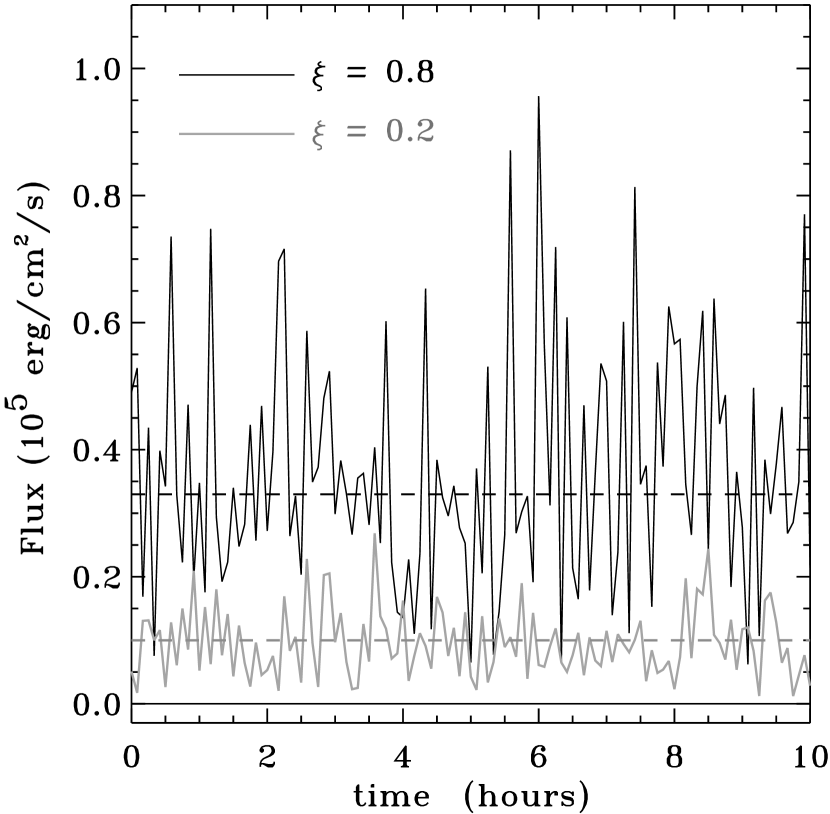
Figure 12.— Time evolution of the energy flux $F_{\rm co}$ released by reconnection into open-field regions, for BONES models having $\xi=0.2$ (gray curves) and $\xi=0.8$ (black curves). Time averages for both cases are denoted by dashed lines.

It is worthwhile to list some of the ways in which the above models may be incomplete or incorrect. For example,

1. The assumption of a succession of potential fields is likely to limit the verisimilitude of the models. It is clear that time dependent, three-dimensional MHD models—which contain currents, resistivity, and finite-pressure effects—would shed more light on the dynamics and energetics of this system. If the gas pressure in localized reconnection regions begins to exceed the magnetic pressure (i.e., $\beta\gtrsim 1$), there may be additional ways for the flux tubes to “break open” that were not accounted for here.

2. Even within the confines of a succession of potential fields, the assumptions of the MCC model may be too simplistic. For example, it is known that in three-dimensional reconnection there are both spatial and temporal variations of the current along separators, which our implementation of MCC does not include (e.g., Galsgaard & Parnell, 2005; Parnell et al., 2010).

3. Our assumption of $\theta_{\rm L}=1$ in Equation (27) may be too large, and thus our resulting estimate for the energy flux released by reconnection may be too high.

4. The simple three-pole magnetic geometry discussed in the Appendix did not consider realistic asymmetries in either the footpoint locations or the magnitudes of the flux sources. When such asymmetries are included (Al-Hachami & Pontin, 2010), the resulting range of values for $C_{\rm L}$ would likely be different. It is unclear whether $C_{\rm L}$ would be larger or smaller than the values estimated in the Appendix.

5. The use of the mean flux element separation $\langle d\rangle$ in Equation (27) is only a rough approximation. Since there may be significant energy release when one flux element gets very close to another, it may be better to use a mean distance that is smaller than $\langle d\rangle$. In that case, our estimate for the heating rate could be too low.

6. As we mentioned in Section 5.1 above, many of the flux tubes that are classified as “open” may in fact be closed in the form of hydrostatic helmet streamers. In reality, then, the energy flux that escapes out into the solar wind could be even lower than the values of $\langle F_{\rm co}\rangle$ that were shown in Figure 11(a). It is also possible that large-scale interchange reconnection could eventually open up these flux tubes (Wang et al., 2000; Fisk, 2005; Antiochos et al., 2010; Edmondson et al., 2010a), but modeling those processes is beyond the scope of this paper.

Roughly speaking, there appear to be just as many reasons why our results for the rates of RLO heating and flux-opening may be overestimates as there are reasons why they may be underestimates. Despite the approximate nature of these models, however, we believe that the main result (i.e., $\langle F_{\rm co}\rangle\ll S$ for most values of $\xi$) is not likely to be wrong by many orders of magnitude.

6. Discussion and Conclusions

The primary aim of this paper was to begin testing the conjecture that the opening up of closed flux in the Sun’s magnetic carpet is responsible for driving the solar wind. First, we created Monte Carlo simulations of the complex photospheric sources of the solar magnetic field. The resulting time-averaged properties of the models appeared to agree well not only with observations of the flux density and the flux imbalance ratio, but also with observed probability distributions for the flux elements and autocorrelation functions of the field strength. A supergranular pattern of network magnetic concentrations appeared spontaneously in the models, despite the lack of any imposed supergranular motions. Then, armed with some degree of confidence that the model photosphere is an adequate reflection of reality, we then computed the coronal magnetic field. Assuming that the coronal field evolves as a succession of potential-field extrapolations, we were able to estimate both the time scales and energy fluxes associated with RLO-type flux-opening events.

From the simulations, we found that the Poynting flux in emerging magnetic elements (which could be a proxy for the maximum energy flux available for coronal heating) is typically around $10^{6}$ erg cm^-2 s^-1. However, for quiet regions ($\xi\ll 1$), only a tiny fraction of the available Poynting flux was found to be released in flux-opening events via magnetic reconnection. A similar situation was found to exist in mixed-polarity regions that can correspond to either quiet Sun or coronal holes ($\xi\lesssim 0.8$). For the most unbalanced coronal hole regions ($\xi\approx 1$), the fraction of Poynting flux released in flux-opening events may approach unity. In these regions, however, the time scale for flux opening was found to be significantly longer than the solar wind travel time from the coronal base to heights far above the tops of loops. Thus, it appears that a significant amount of mass accelerates out into the solar wind over the time that it would take for the plasma to be processed via RLO type mechanisms. From the above estimates of time scales and MCC energetics, we conclude that it is unlikely that the solar wind is driven by reconnection and loop-opening processes in the magnetic carpet.

Despite the negative conclusion regarding the solar wind as a whole, we believe that the physical processes modeled in this paper are likely to be relevant in many other ways. For example, it is possible that more can be learned about the energetics of polar jets with the methodology developed here. Soft X-ray observations can be used to estimate the energy flux released due to jet eruptions. These jets are believed to span several orders of magnitude in the total amount of energy released; i.e., between about $10^{26}$ and $10^{29}$ erg (Shimojo et al., 1998; Chifor et al., 2008; Pariat et al., 2009; Morita et al., 2010). Let us take a canonical value of $E_{\rm jet}\approx 4\times 10^{28}$ erg from the model of Shimojo et al. (1998). Recently, Savcheva et al. (2007) identified 104 jets with the Hinode X-Ray Telescope (XRT) over a time span of 44 hours in a polar coronal hole, which gives a mean time between jets (for the observed area) of $\tau_{\rm jet}\approx 1500$ s. The area examined by Savcheva et al. (2007) was approximately the “front half” of the polar cap, viewed from the side, which extended down to about 25° colatitude and thus covered about $A_{\rm jet}\approx 1.5\times 10^{21}$ cm². Thus, we estimate the mean energy flux released in jets to be $F_{\rm jet}\approx E_{\rm jet}/(A_{\rm jet}\tau_{\rm jet})\approx 2\times 10^{4}$ erg cm^-2 s^-1. This agrees reasonably well with the predicted energy fluxes (for $\xi\approx 0.6$–0.9) shown in Figure 11(a).

The flux-opening events modeled in this paper may also be relevant to understanding the small eruptions seen in quiet regions (Innes et al., 2009; Schrijver, 2010) that may be related to coronal mass ejections (CMEs). However, it is not guaranteed that every jet-like eruption observed in the corona releases material that accelerates up into the solar wind. There is observational evidence that at least some coronal jets contain plasma that falls back down because it failed to reach the escape speed (Baker et al., 2008; Scullion et al., 2009). This may put some jets into the same category as spicules, which are known to carry orders of magnitude more mass up (and down) than is needed to feed the solar wind (e.g., Sterling, 2000; De Pontieu et al., 2009).

A potentially valuable set of observational diagnostics of the processes discussed in this paper are the elemental abundances and ionization states of different particle species that escape into the solar wind (Zurbuchen, 2007). The closed-to-open reconnection events that we have modeled may inject some plasma with a distinctly “closed” composition signature into regions that have signatures otherwise dominated by flux tubes that remain open. It is worth noting, however, that there remains disagreement about exactly what kinds of abundance and ionization signatures signal the presence of closed loops, and which do not. Cranmer et al. (2007) showed that a range of WTD-type open-flux-tube models can produce values of the commonly measured O⁷⁺/O⁶⁺ and Fe/O ratios that agree reasonably well with in situ measurements (see also Pucci et al., 2010). Thus, we question the popular assertion that the charge-state and first-ionization-potential (FIP) properties measured in the slow solar wind can only be explained by the injection of plasma from closed-field regions on the Sun.

Whether or not the solar wind energy budget is accounted for by RLO processes, the inherent variability in the magnetic carpet is likely to cause some kind of MHD fluctuations to propagate up into the corona. The response of the coronal field to the evolving footpoints may result in Alfvén waves with periods of order $\tau_{\rm em}\approx\tau_{\rm co}$ (see Figure 10). In fact, Hollweg (1990, 2008) suggested that “flux cancellation” events in the corona may be the most likely source of the long-period (i.e., 0.5–10 hour) Alfvén waves that dominate in situ measurements. The statistical properties of these low-frequency fluctuations may also be consistent with an origin in the motions of coronal field-line footpoints (Matthaeus & Goldstein, 1986; Giacalone & Jokipii, 2004; Nicol et al., 2009).

In order to further test the applicability of RLO-type processes to accelerating the solar wind, the models need to evolve beyond the approximate potential-field “skeleton” and to incorporate MHD effects. Multi-dimensional MHD simulations (e.g., Gudiksen & Nordlund, 2005; Moreno-Insertis et al., 2008; von Rekowski & Hood, 2008; Edmondson et al., 2009) illustrate the aspects of coronal reconnection that are—and are not—modeled well by potential fields, and future studies need to account for these effects more consistently. Also, analytic models of the micro-scale kinetic physics should be developed further in order to complement the coarser-gridded numerical simulations. Ideas such as stochastic growth theory (Cairns & Robinson, 1998) or non-modal stability (Camporeale et al., 2010) may be useful ways to understand the partitioning of energy within reconnection regions.

Additional work should be done to refine and test the idea that the supergranular network is the natural by-product of smaller-scale granular activity (Rast, 2003). Our success in reproducing the measured autocorrelation patterns in magnetograms (see Figure 5) does not necessarily imply that there is no convective component to supergranulation. However, our results do appear to provide evidence that at least some of the 10–30 Mm magnetic structure on the Sun can be built up from $\sim$1 Mm granulation effects via a kind of diffusion-limited aggregation (see also Crouch et al., 2007).

Another topic that requires further study is the coupling between waves and flux emergence in the granular convective flows at the photospheric lower boundary. Cranmer & van Ballegooijen (2005) estimated that the surface-averaged energy flux of Alfvén waves in the low corona is of order $10^{6}$ erg cm^-2 s^-1 (see Figure 12 of Cranmer & van Ballegooijen, 2005). It is probably not a coincidence that this is of the same order of magnitude as the Poynting flux $S$ due to the emergence of ephemeral regions. The interplay between convective overturning motions, colliding granular cells, and thin flux tubes may give rise to a rough equipartition between these different sources of energy. By constructing models that contain the seeds of both WTD and RLO processes, we can better determine their relative contributions to coronal heating and solar wind acceleration.

Appendix A An Idealized Application of Longcope’s MCC Model for Anemone-Type Events

In this section we show how the Longcope (1996) MCC model can be applied to the results of the BONES simulations described above. In this model, the motions of discrete flux sources on the solar surface give rise to stresses in the coronal field that are concentrated at topological boundaries (i.e., separatrix surfaces and separator field lines). Electric currents are assumed to form along the separators, and then dissipate as magnetic reconnection occurs in response to the evolution of the flux domains. Longcope (1996) found that the power dissipated in a single flux transfer event must be choppy and intermittent, but its time average can be written as

$$\bar{P}\,=\,\theta_{\rm L}\frac{I^{\ast}}{2c}\left|\frac{d\Phi}{dt}\right|\,\,,$$ (A1)

where $d\Phi/dt$ is the time derivative of magnetic flux that is in the process of transferring its connectivity, $I^{\ast}$ is a characteristic current that is assumed to flow along the separator, $\theta_{\rm L}$ is a dimensionless threshold constant describing the intermittency of reconnection, and $c$ is the speed of light in vacuum.

In the double-bipole configuration of Longcope (1996), the transfer of magnetic flux ($d\Phi/dt$) occurred because a fraction of the flux from the positive pole of one bipole became reconnected with the negative pole of the other bipole. In our model, we consider the transfer of flux from a closed flux tube to an open flux tube, or from open to closed. Equation (B9) of Longcope (1996) gave the characteristic current used in Equation (A1) above. Correcting a typographical error in Longcope (1996), this current is given by

$$I^{\ast}\,=\,\frac{c\bar{B}_{\perp}^{\prime}L^{2}s}{8\pi^{2}}$$ (A2)

where $L$ is the length of the separator field line, $s$ is a dimensionless geometrical constant (with $s=1$ corresponding to a circularly shaped separator field line), and $\bar{B}_{\perp}^{\prime}$ is an average value of the Jacobian-like perpendicular derivative of the vector field at the separator,

$$B_{\perp}^{\prime}\,=\,\sqrt{-\mbox{det}\left(\nabla_{\perp}{\bf B}_{\perp}\right)}\,\,.$$ (A3)

In the above, the perpendicular direction is defined relative to the separator field line.

For a given magnetic configuration, the above equations let us estimate the power emitted from the loss of magnetic free energy via reconnection. However, it would be too computationally intensive to locate and trace all of the separator field lines during every time step of the BONES simulation. Thus, we aim to simplify the application of Equation (A1) by creating a characteristic “building block” for the magnetic geometry in a typical (anemone-type) opening/closing event. These building blocks can then be assembled together in a statistical way to account for the total amount of evolving flux in each time step of the Monte Carlo simulations.

Wang (1998) described a simple model of plume/jet events in coronal holes that involved only three discrete flux sources: two that form a localized bipole and a third that represents a unipolar source of open field. As discussed in Section 5.5, the energy release that is assumed to occur in this system happens when some of the flux in the bipole reconnects with the unipolar region, giving rise to an equal amount of opening and closing of flux ($f_{\rm co}=f_{\rm oc}$). For geometric simplicity, let us assume that all three flux sources are collinear along the $x$ axis, with a negative source in between two positive sources. The flux evolution occurs as the negative pole of the bipole moves away from its original positive partner and towards the positive source of open field. We want to evaluate the properties of this system at a representative time in the middle of its evolution, so let us posit an additional symmetry; i.e., we assume that the negative pole sits at the origin ($x=0$) and the two positive poles are both equidistant from the origin ($x=\pm d$) and of equal positive flux. This may be an extreme simplification, since it is known that many details of three-dimensional null-point reconnection do depend on whether the geometry is symmetric or asymmetric (Al-Hachami & Pontin, 2010). However, the other uncertainties in the order-of-magnitude MCC model are probably not outweighed by this issue.

To evaluate the coronal magnetic field arising from this three-pole system, we set the flux in the positive poles to $\Phi_{+}>0$ and flux in the negative pole at the origin to $\Phi_{-}<0$. The two free parameters that constrain the topology of the field lines are the pole separation $d$ and the ratio of negative to positive fluxes $m=|\Phi_{-}/\Phi_{+}|$. Thus, Equation (12) gives

$$B_{x}(x,y,z)=\frac{\Phi_{+}}{2\pi}\left\{\frac{x+d}{[(x+d)^{2}+y^{2}+z^{2}]^{3/2}}+\frac{x-d}{[(x-d)^{2}+y^{2}+z^{2}]^{3/2}}-\frac{mx}{[x^{2}+y^{2}+z^{2}]^{3/2}}\right\}\,\,,$$ (A4)

$$B_{y}(x,y,z)=\frac{\Phi_{+}}{2\pi}\left\{\frac{y}{[(x+d)^{2}+y^{2}+z^{2}]^{3/2}}+\frac{y}{[(x-d)^{2}+y^{2}+z^{2}]^{3/2}}-\frac{my}{[x^{2}+y^{2}+z^{2}]^{3/2}}\right\}\,\,,$$ (A5)

$$B_{z}(x,y,z)=\frac{\Phi_{+}}{2\pi}\left\{\frac{z}{[(x+d)^{2}+y^{2}+z^{2}]^{3/2}}+\frac{z}{[(x-d)^{2}+y^{2}+z^{2}]^{3/2}}-\frac{mz}{[x^{2}+y^{2}+z^{2}]^{3/2}}\right\}\,\,.$$ (A6)

We will consider values of the flux ratio $m$ between about 0.5 and 2. For $m>2$, the central source “breaks out” with its own open field of negative polarity, which is a situation that we are not considering here.

Figure 13(a) illustrates a few representative field lines for the case $m=0.8$. For simplicity, we assume the poles are at $z=0$. The coronal volume ($z>0$) can be separated into four distinct domains according to the field-line topology: (1) a set of open field lines that originates from the left-hand positive pole, (2) a set of open field lines that originates from the right-hand positive pole, (3) a set of closed field lines that connects the left and center poles, and (4) a set of closed field lines that connects the center and right poles. There are two separatrix surfaces that delineate the boundaries between these domains: a vertical surface that spans the $y$–$z$ plane and is defined by the condition $x=0$, and the upper half of a prolate spheroidal surface centered on the origin. The separator field line is the intersection of the two separatrix surfaces, and for this model it is a semicircle in the $y$–$z$ plane.

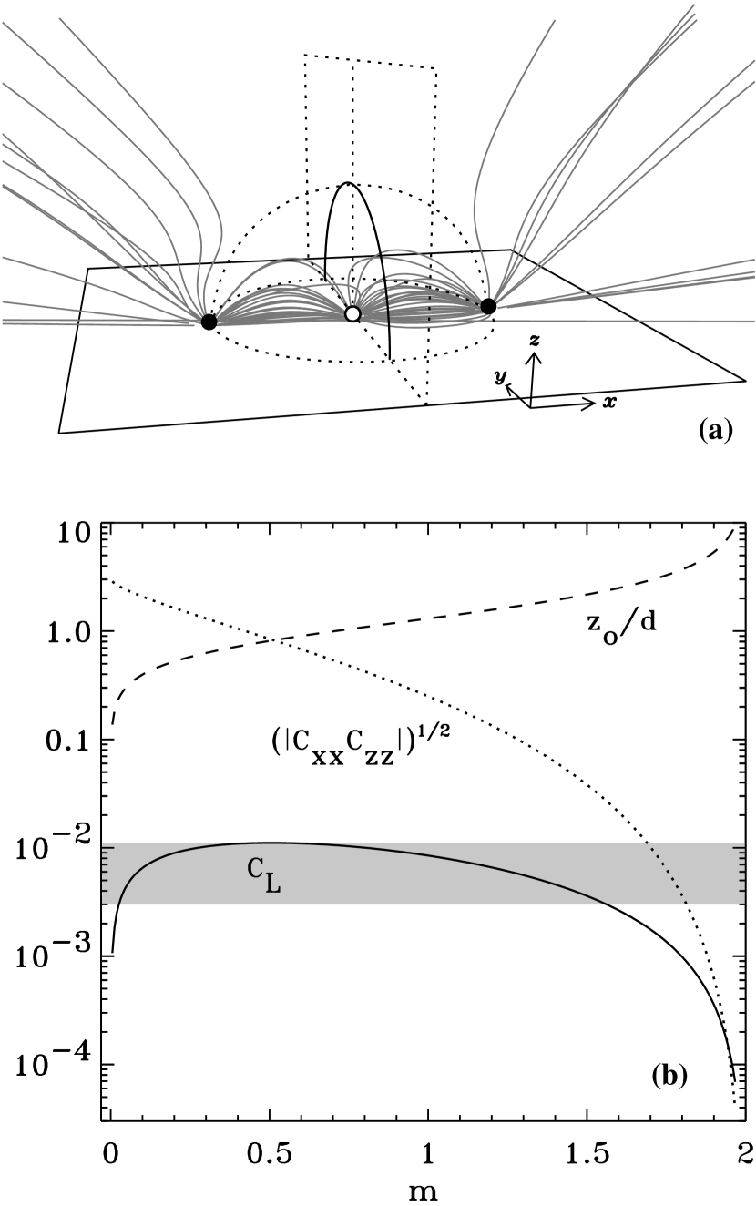
Figure 13.— Properties of the simple three-pole geometry used to estimate several factors in the MCC model. (a) Three-dimensional projection of selected field lines (gray curves), shown along with the two positive poles (filled circles) and the negative pole (open circle) on the surface, the separator field line (black solid curve), and outlines of the locations of the separatrix surfaces (dotted curves). (b) Plot that shows how the null-point height $z_{0}/d$ (dashed curve), the magnetic Jacobian factor $(|C_{xx}C_{zz}|)^{1/2}$ (dotted curve), and the constant $C_{\rm L}$ (solid curve) depend on the flux imbalance ratio $m$. The range of values for $C_{\rm L}$ used when analyzing the results of the BONES models is shown as a gray band.

In order to solve Equation (A3) we need to evaluate the exact position of the separator. First, we locate its maximum height $z_{0}$ by looking for the height of the magnetic null point along the vertical line denoted by $x=0$ and $y=0$. We use Equations (A4)–(A6) to solve for the magnitude of the magnetic field strength, but we do not worry about its absolute normalization. Along the vertical line in question, $B_{x}=B_{y}=0$, and we find that

$$B_{z}\,\propto\,\frac{2}{(d^{2}+z^{2})^{3/2}}-\frac{m}{z^{3}}\,\,.$$ (A7)

We set $B_{z}=0$ and search for a nontrivial solution for $z_{0}>0$. This is a cubic polynomial equation, and Figure 13(b) shows the numerical solution for the ratio $z_{0}/d$ as a function of $m$. Solutions exist only for $m<2$. Due to the symmetry in our assumed system, the separator field line is confined to the plane $x=0$, and it subtends a semicircular shape for $y\neq 0$. Thus, the separator obeys $y^{2}+z^{2}=z_{0}^{2}$, its length is $L=\pi z_{0}$, and we can use the geometrical factor $s=1$ in Equation (A2).

We estimate the average value of $\bar{B}_{\perp}^{\prime}$ along the separator by just computing its value at the maximum height ($x=y=0$, $z=z_{0}$). At this point, the field’s parallel direction points along the $y$ axis, so Equation (A3) can be written

$$\bar{B}_{\perp}^{\prime}\,=\,\sqrt{\left|\frac{\partial B_{x}}{\partial x}\frac{\partial B_{z}}{\partial z}-\frac{\partial B_{z}}{\partial x}\frac{\partial B_{x}}{\partial z}\right|}\,\,.$$ (A8)

The cross-derivatives in the second term are found to be zero, and it can be shown that

$$\bar{B}_{\perp}^{\prime}\,=\,\frac{\Phi_{+}}{\pi d^{3}}\sqrt{|C_{xx}C_{zz}|}\,\,,$$ (A9)

where

$$C_{xx}\,=\,\frac{x-2}{(x+1)^{5/2}}-\frac{m}{2x^{3/2}}$$ (A10)

$$C_{zz}\,=\,\frac{1-2x}{(x+1)^{5/2}}+\frac{m}{x^{3/2}}$$ (A11)

and $x=(z_{0}/d)^{2}$. The two dimensionless factors given in Equations (A10) and (A11) are related to Equation (A8) via

$$\frac{\partial B_{x}}{\partial x}=\frac{\Phi_{+}}{\pi d^{3}}C_{xx}\,\,,\,\,\,\,\,\frac{\partial B_{z}}{\partial z}=\frac{\Phi_{+}}{\pi d^{3}}C_{zz}\,\,.$$ (A12)

Figure 13(b) shows the dimensionless factor $(|C_{xx}C_{zz}|)^{1/2}$ as a function of the flux imbalance ratio $m$.

The above model gives us the ability to write the average power dissipated (Equation (A1)) as

$$\bar{P}\,=\,\theta_{\rm L}C_{\rm L}\frac{\Phi_{+}}{d}\left|\frac{d\Phi}{dt}\right|\,\,,$$ (A13)

where the dimensionless factors dependent on $m$ have been collected into a single constant

$$C_{\rm L}\,=\,\frac{1}{16\pi}\sqrt{|C_{xx}C_{zz}|}\left(\frac{z_{0}}{d}\right)^{2}\,\,.$$ (A14)

Figure 13(b) shows that $C_{\rm L}$ varies less strongly as a function of $m$ than either of its components. In our models, we will not keep track of the individual $m$ imbalance ratios for each reconnection event. Instead we adopt a range of values for $C_{\rm L}$ that spans the majority of the variation for many likely $m$ values. The gray region in Figure 13(b) shows this range of values; the lower limit is 0.003, and the upper limit is the maximum value of 0.011.

The other dimensionless constant in Equation (A1) is $\theta_{\rm L}$. This parameter is a threshold ratio of the instantaneous current density to the characteristic current $I^{\ast}$, and in the MCC model it is assumed that plasma instabilities (e.g., the ion-acoustic instability or tearing-mode instabilities) will limit the growth of the current to some fraction of $I^{\ast}$. Longcope (1996) argued that $\theta_{\rm L}\ll 1$ was reasonable to expect, and he ended up using $\theta_{\rm L}=0.15$ in the initial MCC models. However, Longcope & Silva (1998) and Longcope & Kankelborg (1999) found that some situations appear to demand larger values of order $\theta_{\rm L}\approx 1$. We will use the latter value, but we will keep in mind that the resulting heating rate may be an upper limit.

To apply the heating rate derived above to our Monte Carlo models, we note that Equation (16) gives the time derivative of magnetic flux that is being opened up in the simulation box, during each time step. In order to solve Equation (A13), however, we also need to know the characteristic fluxes in the elements that are interacting, as well as their inter-element distances. Since many reconnection events may be occurring simultaneously in each time step, we must use averages taken over the box area. We also divide both sides of Equation (A13) by $A$ in order to express the heating rate per unit area in terms of the variations in magnetic flux density. Thus,

$$\langle F_{\rm co}\rangle\,=\,\theta_{\rm L}C_{\rm L}\frac{\Phi_{1}}{\langle d\rangle}\left|\frac{dB}{dt}\right|_{\rm co}$$ (A15)

where $\Phi_{1}=\Phi_{\rm abs}/N$ is the mean absolute flux per element in the simulation box, and

$$\langle d\rangle\,=\,\sqrt{\frac{4A}{\pi N}}$$ (A16)

is the mean separation between flux elements. This is the form of the MCC energy flux used for the BONES results presented in Section 5.5.

References

- Abramenko et al. (2009) Abramenko, V., Yurchyshyn, V., & Watanabe, H. 2009, Sol. Phys., 260, 43
- Al-Hachami & Pontin (2010) Al-Hachami, A. K., & Pontin, D. I. 2010, A&A, 512, A84
- Amari et al. (2005) Amari, T., Luciani, J. F., & Aly, J. J. 2005, ApJ, 629, L37
- Antiochos et al. (2007) Antiochos, S. K., DeVore, C. R., Karpen, J. T., & Mikić, Z. 2007, ApJ, 671, 936
- Antiochos et al. (2010) Antiochos, S. K., Mikić, Z., Lionello, R., Titov, V., & Linker, J. 2010, ApJ, submitted
- Aschwanden (2008) Aschwanden, M. J. 2008, in IAU Symp. 247, Waves and Oscillations in the Solar Atmosphere: Heating and Magneto-Seismology, ed. R. Erdélyi & C. Mendoza-Briceño (Cambridge: Cambridge U. Press), 257
- Asensio Ramos (2009) Asensio Ramos, A. 2009, A&A, 494, 287
- Axford & McKenzie (1992) Axford, W. I., & McKenzie, J. F. 1992, in Solar Wind Seven, ed. E. Marsch & R. Schwenn (New York: Pergamon), 1
- Baker et al. (2008) Baker, D., van Driel-Gesztelyi, L., Kamio, S., Culhane, J. L., Harra, L. K., Sun, J., Young, P. R., & Matthews, S. A. 2008, in ASP Conf. Proc. 397, First Results From Hinode, ed. S. Matthews, J. Davis, & L. Harra (San Francisco: ASP), 23
- Banaszkiewicz et al. (1998) Banaszkiewicz, M., Axford, W. I., & McKenzie, J. F. 1998, A&A, 337, 940
- Berger et al. (1998) Berger, T. E., Löfdahl, M. G., Shine, R. A., & Title, A. M. 1998, ApJ, 506, 439
- Berger & Title (1996) Berger, T. E., & Title, A. M. 1996, ApJ, 463, 365
- Beveridge & Longcope (2006) Beveridge, C., & Longcope, D. W. 2006, ApJ, 636, 453
- Bhattacharjee (2004) Bhattacharjee, A. 2004, ARA&A, 42, 365
- Bruno & Carbone (2005) Bruno, R., & Carbone, V. 2005, Living Rev. Solar Phys., 2, 4
- Bryans et al. (2010) Bryans, P., Young, P. R., & Doschek, G. A. 2010, ApJ, 715, 1012
- Buchlin & Velli (2007) Buchlin, E., & Velli, M. 2007, ApJ, 662, 701
- Cadavid et al. (1999) Cadavid, A. C., Lawrence, J. K., & Ruzmaikin, A. A. 1999, ApJ, 521, 844
- Cairns & Robinson (1998) Cairns, I. H., & Robinson, P. A. 1998, ApJ, 509, 471
- Camporeale et al. (2010) Camporeale, E., Passot, T., & Burgess, D. 2010, ApJ, 715, 260
- Chifor et al. (2008) Chifor, C., et al. 2008, A&A, 491, 279
- Close et al. (2005) Close, R. M., Parnell, C. E., Longcope, D. W., & Priest, E. R. 2005, Sol. Phys., 231, 45
- Close et al. (2003) Close, R. M., Parnell, C. E., Mackay, D. H., & Priest, E. R. 2003, Sol. Phys., 212, 251
- Cranmer (2009) Cranmer, S. R. 2009, Living Rev. Solar Phys., 6, 3
- Cranmer (2010) Cranmer, S. R. 2010, ApJ, 710, 676
- Cranmer & van Ballegooijen (2005) Cranmer, S. R., & van Ballegooijen, A. A. 2005, ApJS, 156, 265
- Cranmer et al. (2007) Cranmer, S. R., van Ballegooijen, A. A., & Edgar, R. J. 2007, ApJS, 171, 520
- Crouch et al. (2007) Crouch, A. D., Charbonneau, P., & Thibault, K. 2007, ApJ, 662, 715
- De Pontieu et al. (2009) De Pontieu, B., McIntosh, S. W., Hansteen, V. H., & Schrijver, C. J. 2009, ApJ, 701, L1
- De Rosa & Toomre (2004) De Rosa, M. L., & Toomre, J. 2004, ApJ, 616, 1242
- Deubner & Gough (1984) Deubner, F.-L., & Gough, D. 1984, ARA&A, 22, 593
- Dowdy et al. (1986) Dowdy, J. F., Jr., Rabin, D., & Moore, R. L. 1986, Sol. Phys., 105, 35
- Edmondson et al. (2010a) Edmondson, J. K., Antiochos, S. K., DeVore, C. R., Lynch, B. J., & Zurbuchen, T. H. 2010a, ApJ, 714, 517
- Edmondson et al. (2010b) Edmondson, J. K., Antiochos, S. K., DeVore, C. R., & Zurbuchen, T. H. 2010b, ApJ, 718, 72
- Edmondson et al. (2009) Edmondson, J. K., Lynch, B. J., Antiochos, S. K., DeVore, C. R., & Zurbuchen, T. H. 2009, ApJ, 707, 1427
- Einaudi et al. (1999) Einaudi, G., Boncinelli, P., Dahlburg, R. B., & Karpen, J. T. 1999, J. Geophys. Res., 104, 521
- Fang et al. (2010) Fang, F., Manchester, W., Abbett, W. P., & van der Holst, B. 2010, ApJ, 714, 1649
- Feldman et al. (1999) Feldman, U., Widing, K. G., & Warren, H. P. 1999, ApJ, 522, 1133
- Filippov et al. (2009) Filippov, B., Golub, L., & Koutchmy, S. 2009, Sol. Phys., 254, 259
- Fisk (2003) Fisk, L. A. 2003, J. Geophys. Res., 108, 1157
- Fisk (2005) Fisk, L. A. 2005, ApJ, 626, 563
- Fisk et al. (1999) Fisk, L. A., Schwadron, N. A., & Zurbuchen, T. H. 1999, J. Geophys. Res., 104, 19765
- Fujimoto & Machida (2006) Fujimoto, K., & Machida, S. 2006, J. Geophys. Res., 111, A09216
- Galsgaard (2006) Galsgaard, K. 2006, Adv. Space Res., 37, 1323
- Galsgaard & Parnell (2005) Galsgaard, K., & Parnell, C. E. 2005, A&A, 439, 335
- Giacalone & Jokipii (2004) Giacalone, J., & Jokipii, J. R. 2004, ApJ, 616, 573
- Gloeckler et al. (2003) Gloeckler, G., Zurbuchen, T. H., & Geiss, J. 2003, J. Geophys. Res., 108, 1158
- Goldbaum et al. (2009) Goldbaum, N., Rast, M. P., Ermolli, I., Sands, J. S., & Berrilli, F. 2009, ApJ, 707, 67
- Grappin et al. (2008) Grappin, R., Aulanier, G., & Pinto, R. 2008, A&A, 490, 353
- Gudiksen & Nordlund (2005) Gudiksen, B. V., & Nordlund, Å. 2005, ApJ, 618, 1020
- Guglielmino et al. (2008) Guglielmino, S. L., Zuccarello, F., Romano, P., & Bellot Rubio, L. R. 2008, ApJ, 688, L111
- Hagenaar (2001) Hagenaar, H. J. 2001, ApJ, 555, 448
- Hagenaar et al. (2008) Hagenaar, H. J., De Rosa, M. L., & Schrijver, C. J. 2008, ApJ, 678, 541
- Hagenaar et al. (2010) Hagenaar, H. J., De Rosa, M. L., & Schrijver, C. J. 2010, ApJ, 715, 696
- Hagenaar et al. (1997) Hagenaar, H. J., Schrijver, C. J., & Title, A. M. 1997, ApJ, 481, 988
- Hagenaar et al. (1999) Hagenaar, H. J., Schrijver, C. J., Title, A. M., & Shine, R. A. 1999, ApJ, 511, 932
- Hammer (1982) Hammer, R. 1982, ApJ, 259, 767
- Hansteen (2007) Hansteen, V. H. 2007, in ASP Conf. Proc. 369, New Solar Physics with Solar-B Mission, ed. K. Shibata, S. Nagata, & T. Sakurai (San Francisco: ASP), 193
- Hansteen & Leer (1995) Hansteen, V. H., & Leer, E. 1995, J. Geophys. Res., 100, 21577
- Harra et al. (2008) Harra, L. K., Sakao, T., Mandrini, C. H., Hara, H., Imada, S., Young, P. R., van Driel-Gesztelyi, L., & Baker, D. 2008, ApJ, 676, L147
- Harvey & Martin (1973) Harvey, K. L., & Martin, S. F. 1973, Sol. Phys., 32, 389
- Hirzberger (2002) Hirzberger, J. 2002, A&A, 392, 1105
- Hollweg (1986) Hollweg, J. V. 1986, J. Geophys. Res., 91, 4111
- Hollweg (1990) Hollweg, J. V. 1990, Comput. Phys. Rep., 12, 205
- Hollweg (2008) Hollweg, J. V. 2008, J. Astrophys. Astron., 29, 217
- Innes et al. (2009) Innes, D. E., Genetelli, A., Attie, R., & Potts, H. E. 2009, A&A, 495, 319
- Isobe et al. (2008) Isobe, H., Proctor, M. R. E., & Weiss, N. O. 2008, ApJ, 679, L57
- Ito et al. (2008) Ito, H., Tsuneta, S., Shiota, D., Tokumaru, M., & Fujiki, K. 2010, ApJ, in press, arXiv:1005.3667
- Jiang et al. (2010) Jiang, J., Cameron, R., Schmitt, D., & Schüssler, M. 2010, ApJ, 709, 301
- Keller et al. (2003) Keller, C. U., Harvey, J. W., & the SOLIS Team 2003, in ASP Conf. Proc. 307, Solar Polarization, ed. J. Trujillo-Bueno & J. Sanchez Almeida (San Francisco: ASP), 13
- Krijger & Roudier (2003) Krijger, J. M., & Roudier, T. 2003, A&A, 403, 715
- Kubo et al. (2010) Kubo, M., Low, B. C., & Lites, B. W. 2010, ApJ, 712, 1321
- Leer et al. (1982) Leer, E., Holzer, T. E., & Flå, T. 1982, Space Sci. Rev., 33, 161
- Leighton et al. (1962) Leighton, R. B., Noyes, R. W., & Simon, G. W. 1962, ApJ, 135, 474
- Lionello et al. (2006) Lionello, R., Linker, J. A., Mikić, Z., & Riley, P. 2006, ApJ, 642, L69
- Lites (2002) Lites, B. W. 2002, ApJ, 573, 431
- Livi et al. (1985) Livi, S. H. B., Wang, J., & Martin, S. F. 1985, Australian J. Phys., 38, 855
- Longcope (1996) Longcope, D. W. 1996, Sol. Phys., 169, 91
- Longcope (2005) Longcope, D. W. 2005, Living Rev. Solar Phys., 2, 7
- Longcope & Kankelborg (1999) Longcope, D. W., & Kankelborg, C. C. 1999, ApJ, 524, 483
- Longcope & Silva (1998) Longcope, D. W., & Silva, A. V. R. 1998, Sol. Phys., 179, 349
- Lynch et al. (2008) Lynch, B. J., Antiochos, S. K., DeVore, C. R., Luhmann, J. G., & Zurbuchen, T. H. 2008, ApJ, 683, 1192
- Lynch et al. (2009) Lynch, B. J., Antiochos, S. K., Li, Y., Luhmann, J. G., & DeVore, C. R. ApJ, 697, 1918
- Malara et al. (2007) Malara, F., Veltri, P., & De Franceschis, M. F. 2007, A&A, 467, 1275
- Martin (1988) Martin, S. F. 1988, Sol. Phys., 117, 243
- Martínez González et al. (2010) Martínez González, M. J., Manso Sainz, R., Asensio Ramos, A., & Bellot Rubio, L. R. 2010, ApJ, 714, L94
- Matsumoto & Shibata (2010) Matsumoto, T., & Shibata, K. 2010, ApJ, 710, 1857
- Matthaeus & Goldstein (1986) Matthaeus, W. H., & Goldstein, M. L. 1986, Phys. Rev. Lett., 57, 495
- Matthaeus et al. (1999) Matthaeus, W. H., Zank, G. P., Oughton, S., Mullan, D. J., & Dmitruk, P. 1999, ApJ, 523, L93
- Moreno-Insertis et al. (2008) Moreno-Insertis, F., Galsgaard, K., & Ugarte-Urra, I. 2008, ApJ, 673, L211
- Morita et al. (2010) Morita, S., Shibata, K., Ueno, S., Ichimoto, K., Kitai, R., & Otsuji, K.-I. 2010, PASJ, in press, arXiv:1002.2143
- Muller & Keil (1983) Muller, R., & Keil, S. L. 1983, Sol. Phys., 87, 243
- Nicol et al. (2009) Nicol, R. M., Chapman, S. C., & Dendy, R. O. 2009, ApJ, 703, 2138
- Nisticò et al. (2009) Nisticò, G., Bothmer, V., Patsourakos, S., & Zimbardo, G. 2009, Sol. Phys., 259, 87
- Pariat et al. (2009) Pariat, E., Antiochos, S. K., & DeVore, C. R. 2009, ApJ, 691, 61
- Parker (1958) Parker, E. N. 1958, ApJ, 128, 664
- Parker (1976) Parker, E. N. 1976, ApJ, 210, 810
- Parker (1988) Parker, E. N. 1988, ApJ, 330, 474
- Parnell (2001) Parnell, C. E. 2001, Sol. Phys., 200, 23
- Parnell (2002) Parnell, C. E. 2002, MNRAS, 335, 389
- Parnell & Galsgaard (2004) Parnell, C. E., & Galsgaard, K. 2004, A&A, 428, 595
- Parnell et al. (2008) Parnell, C. E., Haynes, A. L., & Galsgaard, K. 2008, ApJ, 675, 1656
- Parnell et al. (2010) Parnell, C. E., Haynes, A. L., & Galsgaard, K. 2010, J. Geophys. Res., 115, A02102
- Peter et al. (2006) Peter, H., Gudiksen, B. V., & Nordlund, Å. 2006, ApJ, 638, 1086
- Press et al. (1992) Press, W. H., Teukolsky, S. A., Vetterling, W. T., & Flannery, B. P. 1992, Numerical Recipes in Fortran: The Art of Scientific Computing (Cambridge: Cambridge Univ. Press)
- Priest et al. (2002) Priest, E. R., Heyvaerts, J. F., & Title, A. M. 2002, ApJ, 576, 533
- Pucci et al. (2010) Pucci, S., Lie-Svendsen, Ø., & Esser, R. 2010, ApJ, 709, 993
- Rast (2003) Rast, M. P. 2003, ApJ, 597, 1200
- Regnier (2009) Regnier, S. 2009, Eos Trans. AGU, 90 (52), Fall Meet. Suppl., abstract SH51A-1260
- Rieutord & Rincon (2010) Rieutord, M., & Rincon, F. 2010, Living Rev. Solar Phys., 7, 2
- Roxburgh & Tavakol (1979) Roxburgh, I. W., & Tavakol, R. K. 1979, Sol. Phys., 61, 247
- Ryutova et al. (2003) Ryutova, M., Tarbell, T. D., & Shine. R. 2003, Sol. Phys., 213, 231
- Sánchez Almeida et al. (2010) Sánchez Almeida, J., Bonet, J. A., Viticchié, B., & Del Moro, D. 2010, ApJ, 715, L26
- Sandman et al. (2009) Sandman, A. W., Aschwanden, M. J., De Rosa, M. L., Wülser, J. P., & Alexander, D. 2009, Sol. Phys., 259, 1
- Savcheva et al. (2007) Savcheva, A., et al. 2007, PASJ, 59, S771
- Schrijver (2001) Schrijver, C. J. 2001, ApJ, 547, 475
- Schrijver (2010) Schrijver, C. J. 2010, ApJ, 710, 1480
- Schrijver et al. (1997) Schrijver, C. J., Title, A. M., van Ballegooijen, A. A., Hagenaar, H. J., & Shine, R. A. 1997, ApJ, 487, 424
- Schwadron & McComas (2003) Schwadron, N. A., & McComas, D. J. 2003, ApJ, 599, 1395
- Scullion et al. (2009) Scullion, E., Popescu, M. D., Banerjee, D., Doyle, J. G., & Erdélyi, R. 2009, ApJ, 704, 1385
- Seehafer (1986) Seehafer, N. 1986, Sol. Phys., 105, 223
- Shibata et al. (1992) Shibata, K., Nozawa, S., & Matsumoto, R. 1992, PASJ, 44, 265
- Shibata et al. (2007) Shibata, K., et al. 2007, Science, 318, 5856
- Shimojo et al. (2007) Shimojo, M., Narukage, N., Kano, R., Sakao, T., Tsuneta, S., Shibasaki, K., Cirtain, J. W., Lundquist, L. L., Reeves, K. K., & Savcheva, A. 2007, PASJ, 59, S745
- Shimojo et al. (1998) Shimojo, M., Shibata, K., Yokoyama, T., & Hori, K. 1998, in Solar Jets and Coronal Plumes, ed. T.-D. Guyennel, (Noordwijk, The Netherlands: ESA), ESA SP-421, 163
- Shimojo & Tsuneta (2009) Shimojo, M., & Tsuneta, S. 2009, ApJ, 706, L145
- Simon & Leighton (1964) Simon, G. W., & Leighton, R. B. 1964, ApJ, 140, 1120
- Simon et al. (1995) Simon, G. W., Title, A. M., & Weiss, N. O. 1995, ApJ, 442, 886
- Simon et al. (2001) Simon, G. W., Title, A. M., & Weiss, N. O. 2001, ApJ, 561, 427
- Simon & Weiss (1991) Simon, G. W., & Weiss, N. O. 1991, MNRAS, 252, 1P
- Singh & Bappu (1981) Singh, J., & Bappu, M. K. V. 1981, Sol. Phys., 71, 161
- Stein et al. (2010) Stein, R. F., Lagerfjärd, A., Nordlund, Å., & Georgobiani, D. 2010, Sol. Phys., in press, arXiv:0912.4938
- Sterling (2000) Sterling, A. C. 2000, Sol. Phys., 196, 79
- Subramanian et al. (2010) Subramanian, S., Madjarska, M. S., & Doyle, J. G. 2010, A&A, 516, A50
- Suess & Nerney (2004) Suess, S. T., & Nerney, S. 2004, Adv. Space Res., 33, 668
- Suzuki & Inutsuka (2006) Suzuki, T. K., & Inutsuka, S.-I. 2006, J. Geophys. Res., 111, A06101
- Syrovatskii (1982) Syrovatskii, S. I. 1982, Sol. Phys., 76, 3
- Tian et al. (2010) Tian, H., Tu, C.-Y., Marsch, E., He, J.-S., Zhou, C., & Zhao, L. 2010, in AIP Conf. Proc. 1216, Solar Wind 12, ed. M. Maksimovic, K. Issautier, N. Meyer-Vernet, M. Moncuquet, & F. Pantellini (Melville, NY: AIP), 36
- Title and Schrijver (1998) Title, A. M., & Schrijver, C. J. 1998, in ASP Conf. Proc. 154, 10th Cambridge Workshop on Cool Stars, Stellar Systems and the Sun, ed. R. Donahue & J. Bookbinder (San Francisco: ASP), 345
- Tu & Marsch (1995) Tu, C.-Y., & Marsch, E. 1995, Space Sci. Rev., 73, 1
- van Ballegooijen et al. (1998) van Ballegooijen, A. A., Cartledge, N. P., & Priest, E. R. 1998, ApJ, 501, 866
- van Ballegooijen & Mackay (2007) van Ballegooijen, A. A., & Mackay, D. H. 2007, ApJ, 659, 1713
- Velli et al. (1991) Velli, M., Grappin, R., & Mangeney, A. 1991, Geoph. Astrophys. Fluid Dyn., 62, 101
- Verdini et al. (2010) Verdini, A., Velli, M., Matthaeus, W. H., Oughton, S., & Dmitruk, P. 2010, ApJ, 708, L116
- von Rekowski & Hood (2008) von Rekowski, B., & Hood, A. W. 2008, MNRAS, 385, 1792
- Walsh & Galtier (2000) Walsh, R. W., & Galtier, S. 2000, Sol. Phys., 197, 57
- Wang (1988) Wang, H. 1988, Sol. Phys., 116, 1
- Wang et al. (1996) Wang, H., Tang, F., Zirin, H., & Wang, J. 1996, Sol. Phys., 165, 223
- Wang (1998) Wang, Y.-M. 1998, ApJ, 501, L145
- Wang et al. (2009) Wang, Y.-M., Ko, Y.-K., & Grappin, R. 2009, ApJ, 691, 760
- Wang et al. (1989) Wang, Y.-M., Nash, A. G., & Sheeley, N. R., Jr. 1989, ApJ, 347, 529
- Wang & Sheeley (1991) Wang, Y.-M., & Sheeley, N. R., Jr. 1991, ApJ, 372, L45
- Wang et al. (2000) Wang, Y.-M., Sheeley, N. R., Socker, D. G., Howard, R. A., & Rich, N. B. 2000, J. Geophys. Res., 105, 25133
- Wang et al. (1998) Wang, Y.-M., Sheeley, N. R., Socker, D. G., Howard, R. A., Brueckner, G. E., Michels, D. J., Moses, D., St. Cyr, O. C., Llebaria, A., & Delaboudinière, J. P. 1998, ApJ, 508, 899
- Welsch et al. (2009) Welsch, B. T., Li, Y., Schuck, P. W., & Fisher, G. H. 2009, ApJ, 705, 821
- Wiegelmann & Solanki (2004) Wiegelmann, T., & Solanki, S. K. 2004, Sol. Phys., 225, 227
- Withbroe (1988) Withbroe, G. L. 1988, ApJ, 325, 442
- Withbroe & Noyes (1977) Withbroe, G. L., & Noyes, R. W. 1977, ARA&A, 15, 363
- Yamada (2007) Yamada, M. 2007, Phys. Plasmas, 14, 058102
- Yeates et al. (2010) Yeates, A. R., Attrill, G. D. R., Nandy, D., Mackay, D. H., Martens, P. C. H., & van Ballegooijen, A. A. 2010, ApJ, 709, 1238
- Zhang et al. (2006) Zhang, J., Ma, J., & Wang, H. 2006, ApJ, 649, 464
- Zurbuchen (2007) Zurbuchen, T. H. 2007, ARA&A, 45, 297