3D Euler equations and ideal MHD mapped to regular systems:
probing the finite-time blowup hypothesis

Abstract

We prove by an explicit construction that solutions to incompressible 3D Euler equations defined in the periodic cube $\Omega=[0,L]^{3}$ can be mapped bijectively to a new system of equations whose solutions are globally regular. We establish that the usual Beale-Kato-Majda criterion for finite-time singularity (or blowup) of a solution to the 3D Euler system is equivalent to a condition on the corresponding regular solution of the new system. In the hypothetical case of Euler finite-time singularity, we provide an explicit formula for the blowup time in terms of the regular solution of the new system. The new system is amenable to being integrated numerically using similar methods as in Euler equations. We propose a method to simulate numerically the new regular system and describe how to use this to draw robust and reliable conclusions on the finite-time singularity problem of Euler equations, based on the conservation of quantities directly related to energy and circulation. The method of mapping to a regular system can be extended to any fluid equation that admits a Beale-Kato-Majda type of theorem, e.g. 3D Navier-Stokes, 2D and 3D magnetohydrodynamics, and 1D inviscid Burgers. We discuss briefly the case of 2D ideal magnetohydrodynamics. In order to illustrate the usefulness of the mapping, we provide a thorough comparison of the analytical solution versus the numerical solution in the case of 1D inviscid Burgers equation.

I Introduction

One of the most important unsolved problems in Mathematics entails a simple question: are solutions to the three-dimensional Euler equations globally regular or do they blow up in a finite time? The analogous question for Navier-Stokes equations, also unsolved, corresponds to one of the famous Millennium Prize problems Millennium . The analytical and numerical methods appearing in the scientific literature to solve these equations have been highly transferrable to real-life problems, such as high-Reynolds number turbulence and vortex reconnection in Navier-Stokes, magnetic reconnection in magnetohydrodynamics, and extreme events in the atmosphere, to mention a few.

While several conclusive results are available for Euler and Navier-Stokes in two dimensions, three dimensions with axial symmetry and three dimensions with helical symmetry Yudovich63 ; Kat67 ; Ladyzenskaja68 ; Ukhovskii68 ; Mahalov90 ; Dutrifoy99 ; Ettinger09 , attempts to understand the regularity of three-dimensional solutions have only reached local and/or conditional analytical results Ebi70 ; Kat72 ; Bou74 ; Tem75 ; BKM84 ; Pon85 ; Fer93 ; Cons94 ; Consetal96 ; KozTan00 ; Cor01 ; Dengetal03 ; Cha03 ; Cha04 ; Cha05 ; Dengetal05 ; Dengetal05a ; Chae07 ; Gib07 ; Gib08 . Since the advent of powerful computers circa 1980, numerical researchers have also contributed with competing yes/no conclusions regarding finite-time singularity, mainly in three-dimensional Euler, which is the focus of the present paper Bar76 ; Morf80 ; Cho82 ; Bra83 ; Sig84 ; Kid85 ; Pum87 ; Ash87 ; Pum90 ; Bel92 ; Bra92 ; Ker93 ; Bor94 ; Pel97 ; Gra98 ; Pel01 ; Ker05a ; Pel05 ; Gul05 ; Cich05 ; Ker05 ; Pau06 ; HouLi06 ; Orl07 ; Graf08 ; HouLi08 ; BusKerr08 .

In a 3D Euler numerical simulation the spatial distribution of vorticity tends to get localised in structures that become increasingly sharp with time. This entails a finite-time loss of resolution, not necessarily due to a true finite-time singularity of the solutions, but rather to a finite amount of memory available for a computer simulation. One can identify two main drawbacks in current and previous state-of-the-art numerical attempts on the Euler singularity problem. On the one hand, it is not known analytically whether a given initial condition can give rise to a finite-time singularity, hence a numerical solution of 3D Euler equations is inherently “blind” to any potential finite-time singularity that may be encountered: numerical dissipation and loss of resolution may certainly “shield” the singularity. On the other hand, instability and numerical error could give rise to a “fake” finite-time singularity, typically associated with a lack of resolution at late stages of a simulation.

This observation motivated the current research: our main analytical result is that there is a bijective mapping from Euler equations (along with velocity fields) to a new system of equations, hereby called mapped, whose solutions are globally regular. The mapped system is amenable to direct numerical integration using the same methods as in Euler equations, with the important advantage that the solutions of the mapped system are regular by definition. In this way, and for the first time ever, reliable and robust conclusions on the problem of finite-time singularity of Euler equations could be drawn, by analysing in post-processing the data from a careful numerical integration of the mapped system.

In Section II we define the bijective mapping from 3D Euler to a regular system, provide the proofs of global regularity, and show how to use the solution of the regular system to probe the hypothesis of finite-time singularity of the 3D Euler equations. In Section III we propose a numerical method to implement these ideas and discuss the advantages and potential challenges of the new approach. In Section IV we show that other equations of interest in physics and mathematics can be mapped to regular systems, provided they admit a Beale-Kato-Majda (BKM) type of theorem (e.g., Navier-Stokes, magnetohydrodynamics and inviscid Burgers), and we construct an explicit mapping from the 2D ideal magnetohydrodynamics equations to a regular system. In Section V we illustrate the usefulness of the mapping to a regular system, by considering a simple equation admitting a BKM type of theorem: the 1D inviscid Burgers equation. We compare thoroughly the analytical solution for the supremum norm of velocity gradient, with the numerical data from both direct numerical simulation of inviscid Burgers and numerical simulation of the mapped system, and conclude that the integration of the regular mapped system is far more accurate and converges better than the original system. Finally, we present concluding remarks in Section VI.

II Euler equations: previous vs. novel approach

II.1 Euler equations in a periodic cuboid

The Euler fluid equations describe the evolution of an incompressible, unit mass density flow with velocity field ${\mathbf{u}}(x,y,z,t)\in\mathbb{R}^{3}$ defined for $(x,y,z)\in\mathbb{R}^{3}$ and in a time interval $t\in[0,T)$:

$$\frac{\partial{\mathbf{u}}}{\partial t}+{\mathbf{u}}\cdot\nabla{\mathbf{u}}=-\nabla p\,,\qquad\quad\nabla\cdot{\mathbf{u}}=0.$$ (1)

Periodic boundary conditions are assumed for the velocity field and pressure with a basic periodicity domain $\Omega=[0,L]^{3}$. That is, for any $(x,y,z)\in\mathbb{R}^{3}$ we have ${\mathbf{u}}(x+L,y,z,t)={\mathbf{u}}(x,y+L,z,t)={\mathbf{u}}(x,y,z+L,t)={\mathbf{u}}(x,y,z,t),\,\forall\,t\in[0,T)$ and similarly for $p$. The basic periodicity domain is by definition the smallest domain with such periodicity property.

Here, and throughout this proposal, $T$ denotes a generic time so that ${\mathbf{u}}\in C([0,T);H^{s})\cap C^{1}([0,T);H^{s-1})\,,\,\,s\geq 3\,,$ so in particular the Sobolev norms of the velocity field are bounded:

$${{||{\mathbf{u}}(\cdot,t)||_{H^{s}}\equiv\left({\displaystyle\sum\limits_{{\mathbf{k}}\in\mathbb{Z}^{3}}}(1+|{\mathbf{k}}|^{2})^{s}\,|\widehat{{\mathbf{u}}}({\mathbf{k}},t)|^{2}\right)^{\frac{1}{2}}\leq c_{s}\,,\,\,t\in[0,T)\,,\,\,s\geq 3\,,}}$$ (2)

where $c_{s}$ are some constants and $\widehat{{\mathbf{u}}}({\mathbf{k}},t)$ are the Fourier coefficients of the velocity field.

II.2 Previous analytical and numerical results: vorticity and the finite-time singularity hypothesis

In order to gain some insight on the problem of finite-time blowup, the most common approach is to monitor from numerical simulations a number of quantities pertaining to the theory. The main quantity studied since early numerical simulations (ca. 1987) is the vorticity supremum norm $||\mathbf{\mbox{\boldmath{$\omega$}}}(\cdot,t)||_{\infty}\equiv{\sup_{{\mathbf{x}}\in\Omega}}|\mbox{\boldmath{$\omega$}}({\mathbf{x}},t)|\,,$ where $\mbox{\boldmath{$\omega$}}\equiv\nabla\times{\mathbf{u}}$ is the vorticity field. According to a theorem by Beale, Kato and Majda (BKM) BKM84 , the assumed regularity of the velocity field can be extended up to and including the time $T$ if and only if $\tau(T)\equiv\int_{0}^{T}||\mbox{\boldmath{$\omega$}}(\cdot,t)||_{\infty}~{}dt<\infty.$ By ‘regular up to and including the time $T$’ we mean ${\mathbf{u}}\in C([0,T];H^{s})\cap C^{1}([0,T];H^{s-1}),\,s\geq 3$.

The hypothesis of finite-time singularity (blowup) states that there is a ‘singularity time’ $T\in(0,\infty)$, such that $\tau(T)=\infty.$ It is an open problem to establish analytically the validity of this hypothesis. Consequently, it has been an important aim of many numerical simulations of Euler equations (1), published since BKM theorem emerged, to conclude yes, no or maybe on the validity of this hypothesis. Unfortunately, direct numerical simulations of Euler equations entail an inherent uncertainty about the time of a hypothetical singularity. Therefore, current numerical attempts on the Euler singularity problem cannot give 100% reliable conclusions in favour of or against a finite-time singularity. A fresh approach is urgently needed to continue along this research path.

II.3 The novel approach

The main goal of this paper is to provide such a fresh approach to study the validity of the hypothesis of finite-time singularity. This is based on a bijective mapping which maps the Euler equations to a system whose solutions are globally regular. The mapping from ‘old variables’ $(t,{\mathbf{u}}({\mathbf{x}},t))$ to ‘mapped variables’ $(\tau,{\mathbf{u}}_{\mathrm{map}}({\mathbf{x}},\tau))$ is defined by:

$$\tau(t)\equiv\int_{0}^{t}||\mathbf{\mbox{\boldmath{$\omega$}}}(\cdot,t^{\prime})||_{\infty}~{}dt^{\prime}\,,\qquad{\mathbf{u}}_{\mathrm{map}}({\mathbf{x}},\tau)\equiv\frac{{\mathbf{u}}({\mathbf{x}},t)}{||\mathbf{\mbox{\boldmath{$\omega$}}}(\cdot,t)||_{\infty}}\,.$$ (3)

The mapped time $\tau(t)$ is a strictly monotonically increasing function of $t$ and the mapped velocity is well defined due to the following result:

Lemma 1. Assume the initial vorticity is not identically zero on $\Omega.$ Then the vorticity supremum norm is positive: $||\mathbf{\mbox{\boldmath{$\omega$}}}(\cdot,t)||_{\infty}>0\,,\forall\,t\in[0,T).$ $\square$

Proof. Using the well-known fact that the zeroes of vorticity are preserved by the flow for as long as the vorticity is defined, we get: $||\mathbf{\mbox{\boldmath{$\omega$}}}(\cdot,t_{1})||_{\infty}=0$ for some $t_{1}\in[0,T)$ if and only if $||\mathbf{\mbox{\boldmath{$\omega$}}}(\cdot,t)||_{\infty}=0\,,\,\,\forall\,t\in[0,T).$ Since the initial vorticity is not identically zero, the Lemma follows. $\square$

Moreover, the characteristics of each system are mapped accordingly. Let ${\mathbf{X}}({\mathbf{X}}_{0},t)$ and ${\mathbf{X}}_{\mathrm{map}}({\mathbf{X}}_{0},\tau)$ be the respective solutions of

$$\frac{d}{dt}{\mathbf{X}}({\mathbf{X}}_{0},t)={\mathbf{u}}({\mathbf{X}}({\mathbf{X}}_{0},t),t)\,,\qquad\frac{d}{d\tau}{\mathbf{X}}_{\mathrm{map}}({\mathbf{X}}_{0},\tau)={\mathbf{u}}_{\mathrm{map}}({\mathbf{X}}_{\mathrm{map}}({\mathbf{X}}_{0},\tau),\tau)\,,$$

with initial conditions ${\mathbf{X}}_{\mathrm{map}}({\mathbf{X}}_{0},0)={\mathbf{X}}({\mathbf{X}}_{0},0)={\mathbf{X}}_{0}\,.$ Then, using equations (3) we get ${\mathbf{X}}_{\mathrm{map}}({\mathbf{X}}_{0},\tau(t))={\mathbf{X}}({\mathbf{X}}_{0},t)\,.$

The Euler equations (1) are equivalent to the system:

$$\frac{\partial{\mathbf{u}}_{\mathrm{map}}}{\partial\tau}+{\mathbf{u}}_{\mathrm{map}}\cdot\nabla{\mathbf{u}}_{\mathrm{map}}=-\nabla{p_{\mathrm{map}}}-\beta(\tau)\,{\mathbf{u}}_{\mathrm{map}}\,,\qquad\quad\nabla\cdot{\mathbf{u}}_{\mathrm{map}}=0\,,$$ (4)

where all mapped fields are to be evaluated at $({\mathbf{x}},\tau)$ unless explicitly stated, and the coefficient $\beta(\tau)$ (damping if and only if $\int_{\Omega}|{\mathbf{u}}_{\mathrm{map}}({\mathbf{x}},\tau)|^{2}~{}d^{3}x$ decreases in time) is defined by

$$\beta(\tau)\equiv{\mbox{\boldmath{$\omega$}}_{\mathrm{map}}({\mathbf{Y}}(\tau),\tau)\cdot\left(\nabla{\mathbf{u}}_{\mathrm{map}}({\mathbf{Y}}(\tau),\tau)\right)\cdot\mbox{\boldmath{$\omega$}}_{\mathrm{map}}({\mathbf{Y}}(\tau),\tau)}\,,$$ (5)

where $\mbox{\boldmath{$\omega$}}_{\mathrm{map}}({\mathbf{x}},\tau)\equiv\nabla\times{\mathbf{u}}_{\mathrm{map}}({\mathbf{x}},\tau)$ is the mapped vorticity and ${\mathbf{Y}}(\tau)$ is the position of mapped vorticity maximum, with $|{\mbox{\boldmath{$\omega$}}}_{\mathrm{map}}({\mathbf{x}},\tau)|\leq||{\mbox{\boldmath{$\omega$}}}_{\mathrm{map}}(\cdot,\tau)||_{\infty}=|{\mbox{\boldmath{$\omega$}}}_{\mathrm{map}}({\mathbf{Y}}(\tau),\tau)|=1\,\quad\forall\,\tau,\,\forall\,{\mathbf{x}}\in\Omega\,.$

The existence of ${\mathbf{Y}}(\tau)$ and $\beta(\tau)$ is a consequence of the assumed regularity of the velocity field: ${\mathbf{u}}\in C([0,T);H^{s})\cap C^{1}([0,T);H^{s-1})\,,\,\,s\geq 3\,,$ along with Lemma 1 and a well-known Sobolev lemma:

$$||D^{p}{\mathbf{F}}(\cdot)||_{\infty}\leq\widetilde{c}_{s}\,||{\mathbf{F}}(\cdot)||_{H^{s+p}}\,,\,\forall\,p\in\mathbb{Z}^{+}\cup\{0\},\,s>3/2\,,$$

valid for 3D vector fields ${\mathbf{F}}$ defined on $\Omega$, where $D^{p}$ is any combination of spatial derivatives of combined order $p$.

In order to be able to treat ${\mathbf{Y}}(\tau)$ as a function, a selection mechanism is required. Apart from mirror images –which do not pose any problem for the selection mechanism–, in the generic case ${\mathbf{Y}}(\tau)$ can be taken as a piecewise continuous function, with jumps at times when two competing local spatial maxima of $|{\mbox{\boldmath{$\omega$}}}_{\mathrm{map}}({\mathbf{x}},\tau)|$, located at different places, coincide in value. The full treatment of this generic case of discontinuous ${\mathbf{Y}}(\tau)$ is possible and straightforward. But, for the sake of this paper and to fix ideas, we assume from here on that ${\mathbf{Y}}(\tau)$ is continuous. We remark that the main results discussed in this paper (Theorem 2 and Corollary 3) can be extended with slight modifications to the general case of discontinuous ${\mathbf{Y}}(\tau)$. It is worth mentioning that several initial conditions considered as candidates for finite-time singularity Bra83 ; Ker93 ; HouLi06 ; Kid85 belong to the simplified case of continuous ${\mathbf{Y}}(\tau)$.

The new system (4)–(5) is globally regular:

Theorem 2. The solution of the new system (4)–(5) is regular for all finite values of the mapped time $0\leq\tau<\infty$. $\square$

Proof. Let us suppose $\tau\in[0,\tau_{0}]$ with $0<\tau_{0}<\infty$ fixed. We obtain, using equation (3),

$$\int_{0}^{t^{\prime}}||{\mbox{\boldmath{$\omega$}}}(\cdot,t^{\prime\prime})||_{\infty}~{}dt^{\prime\prime}\leq\tau_{0}<\infty\,,\quad\forall\,t^{\prime}\in[0,t(\tau_{0})]\,,$$

where $t(\tau)$ is the inverse map from new to original time. According to BKM theorem BKM84 , this implies that in original variables all Sobolev norms of velocity $||{\mathbf{u}}(\cdot,t)||_{H^{s}}$ are bounded for all times $t\in[0,t(\tau_{0})]\,.$ Also, by virtue of Lemma 1 the vorticity modulus supremum norm is positive: $||{\mbox{\boldmath{$\omega$}}}(\cdot,t)||_{\infty}>0,t\in[0,t(\tau_{0})]\,.$ Therefore we can transform to the mapped variables and use equation (2) to conclude that all Sobolev norms of mapped velocity $||{\mathbf{u}}_{\mathrm{map}}(\cdot,\tau)||_{H^{s}}=||{\mathbf{u}}(\cdot,t(\tau))||_{H^{s}}/||{\mbox{\boldmath{$\omega$}}}(\cdot,t(\tau))||_{\infty}$ are bounded for $\tau\in[0,\tau_{0}]\,.$ Since $\tau_{0}$ is arbitrary the result ${\mathbf{u}}_{\mathrm{map}}\in C([0,\infty);H^{s})\,,\,\,s\geq 3$ is established. Along similar lines we can show that ${\mathbf{u}}_{\mathrm{map}}\in C^{1}([0,\infty);H^{s-1}).$ The proof is omitted here. $\square$

Theorem 2 holds even if the Euler system (1) has a finite-time singularity. This is very useful from a computational point of view: one is sure that a careful numerical integration of the new system should give rise to a regular solution, and this alone leads to a more reliable test of the validity of the finite-time singularity hypothesis. This is in contrast with numerical simulations of the original Euler equations, where numerical errors and lack of resolution may fail to find true finite-time singularities or may give rise to spurious ones, making any conclusions unreliable.

II.4 A robust criterion for finite-time singularity of Euler system

In the original variables there are two types of constants of motion: the total kinetic energy of the fluid and the circulations of velocity field along selected closed contours. For simplicity we focus on the energy $E\equiv\frac{1}{2}||{\mathbf{u}}(\cdot,t)||_{L^{2}}^{2}=\frac{1}{2}\int_{\Omega}|{\mathbf{u}}({\mathbf{x}},t)|^{2}~{}d^{3}x,$ defined in terms of the $L^{2}$-norm of velocity. In pseudospectral Euler simulations, constancy of energy is very robust and it holds even when small-scale errors pervade the system. In a numerical simulation of the mapped system (4)–(5) we do not have direct access to the Euler energy but we can define the mapped energy:

$$E_{\mathrm{map}}(\tau)\equiv\frac{1}{2}||{\mathbf{u}}_{\mathrm{map}}(\cdot,\tau)||_{L^{2}}^{2}=\frac{1}{2}\int_{\Omega}|{\mathbf{u}}_{\mathrm{map}}({\mathbf{x}},\tau)|^{2}~{}d^{3}x\,,$$ (6)

which is not constant. From (3) we deduce that the supremum norm of the original vorticity $||{\mbox{\boldmath{$\omega$}}}(\cdot,t(\tau))||_{\infty}$ can be obtained in terms of the Euler energy and mapped energy:

$$||{\mbox{\boldmath{$\omega$}}}(\cdot,t(\tau))||_{\infty}=\sqrt{\frac{E}{E_{\mathrm{map}}(\tau)}}\,,$$ (7)

where the implicit inverse transformation $t(\tau)$ appears naturally. Notice that in practical applications, both the original Euler energy $E$ and mapped energy $E_{\mathrm{map}}(\tau)$ are nonzero.

We reconstruct the original time $t(\tau)$ by integrating $dt/d\tau=1/||{\mbox{\boldmath{$\omega$}}}(\cdot,t(\tau))||_{\infty}$ and using (7):

$$t(\tau)=\int_{0}^{\tau}\frac{1}{||{\mbox{\boldmath{$\omega$}}}(\cdot,t(\tau^{\prime}))||_{\infty}}~{}d\tau^{\prime}=\int_{0}^{\tau}\sqrt{\frac{E_{\mathrm{map}}(\tau^{\prime})}{E}}~{}d\tau^{\prime}\,.$$ (8)

This allows us to re-word the BKM criterion for singularity of Euler, in terms of the regular solution of the mapped equations (4)–(5). Let us define the quantity $t_{\mathrm{end}}$:

$$t_{\mathrm{end}}\equiv\int_{0}^{\infty}\sqrt{\frac{E_{\mathrm{map}}(\tau)}{E}}~{}d\tau=\frac{\int_{0}^{\infty}||{\mathbf{u}}_{\mathrm{map}}(\cdot,\tau)||_{L^{2}}~{}d\tau}{||{\mathbf{u}}(\cdot,0)||_{L^{2}}}\,.$$ (9)

Corollary 3. The solution of the 3D Euler system (1) has a finite-time singularity if and only if  $t_{\mathrm{end}}<\infty,$ in which case the singularity is attained at time $t=t_{\mathrm{end}}$ in the original variables. $\square$

This represents a ‘duality’ between the mapped regular system and the original system: a fast decay in time of the mapped field is equivalent to a finite-time blowup of the original field.

III Proposed numerical simulations of mapped system and the finite-time blowup hypothesis of 3D Euler equations

III.1 Advantages of the new approach

The numerical integration of the mapped system (4)–(5) is completely independent of the Euler system (1), and its main advantages are:

Adv. 1. Since the profile of vorticity modulus is always bounded by 1, we expect a better regularity of all fields involved in the computation of the next timestep data: velocity field and damping coefficient $\beta(\tau)$. This will reduce numerical errors.

Adv. 2. As the profile of vorticity becomes more and more pronounced near its maximum (with vorticity modulus equal to 1 at the maximum), the value of vorticity modulus away from the peak tends to zero. Accordingly, all numerical noise generated away from the peak should be damped to zero. This is due to the damping produced by $\beta(\tau)$, defined in equation (5).

Adv. 3. Due to the boundedness of velocity, the Courant condition will produce a timestep which is bounded from below (see Section III.3 for details on the numerical code).

Adv. 4. The new approach puts in the same footing the two potential types of solutions of Euler equations: the ones that are globally regular and the ones that blow up in a finite time. The reason being that for each of the two types, the mapped version is regular. This gives a common platform to study the effect of initial conditions on the singular character of the solutions.

Adv. 5. For solutions of Euler equations that are candidates for finite-time singularity, the integration of the mapped regular equations will get further in time with better accuracy than the direct integration of Euler equations. Once the new numerical codes to solve the mapped equations are validated, our method will serve as a consistency test for the old Euler codes.

III.2 Initial conditions

The guiding principle to set up initial conditions will be to use discrete mirror symmetries, which enable us to reach high resolution by saving memory and computation time. Types of initial conditions to be studied range from Taylor-Green-like to anti-parallel vortices, and we will apply to all these initial conditions a growth-optimisation procedure which is under development. First we set up the initial conditions for the field ${\mathbf{u}}({\mathbf{x}},t)$ at $t=0$: ${\mathbf{u}}({\mathbf{x}},0)={\mathbf{u}}_{0}({\mathbf{x}})$ such that $\nabla\cdot{\mathbf{u}}_{0}({\mathbf{x}})=0\,\,\forall\,{\mathbf{x}}\in\Omega\,.$ We construct the initial vorticity: $\mbox{\boldmath{$\omega$}}_{0}({\mathbf{x}})\equiv\nabla\times{\mathbf{u}}_{0}({\mathbf{x}})\,,$ and compute its supremum norm and the position ${\mathbf{Y}}(0)$ where it attains its maximum value: $||{\mbox{\boldmath{$\omega$}}}_{0}(\cdot)||_{\infty}\equiv\sup_{{\mathbf{x}}\in\Omega}|{\mbox{\boldmath{$\omega$}}}_{0}({\mathbf{x}})|=|{\mbox{\boldmath{$\omega$}}}_{0}({\mathbf{Y}}(0))|\,.$ Finally, we compute the initial energy $E=\frac{1}{2}\int_{\Omega}|{\mathbf{u}}_{0}({\mathbf{x}})|^{2}~{}d^{3}x\,.$

Following the mapping described in Section II.3, we now construct the initial conditions corresponding to the system (4)–(5). Notice that there is no need to explicitly ‘solve’ for $\tau$ as a function of $t$. We merely set $\tau(0)=0\,.$ The initial conditions for the mapped velocity are thus ${\mathbf{u}}_{\mathrm{map}}({\mathbf{x}},0)={{\mathbf{u}}_{0}({\mathbf{x}})}/{||{\mbox{\boldmath{$\omega$}}}_{0}(\cdot)||_{\infty}}\,.$ The mapped vorticity $\mbox{\boldmath{$\omega$}}_{\mathrm{map}}=\nabla\times{\mathbf{u}}_{\mathrm{map}}$ satisfies initially $|\mbox{\boldmath{$\omega$}}_{\mathrm{map}}({\mathbf{x}},0)|\leq 1,\,\forall\,{\mathbf{x}}\in\Omega,$ and $|\mbox{\boldmath{$\omega$}}_{\mathrm{map}}({\mathbf{Y}}(0),0)|=1\,.$

III.3 Numerical integration of the mapped equations

We will integrate numerically the mapped regular system (4)–(5). For this we will modify extensively two existing Euler codes, in order to develop a new code where at each time step the following extra procedures are implemented:

$\bullet$ an accurate modelling of the nonlocal damping coefficient $\beta(\tau)$, equation (5), using a high-order interpolation method to find the instantaneous position ${\mathbf{Y}}(\tau)$ of the maximum of vorticity modulus and then computing the interpolated gradient of velocity at that point;

$\bullet$ a normalisation algorithm that guarantees that the vorticity modulus be exactly equal to 1 at ${\mathbf{x}}={\mathbf{Y}}(\tau),$ as it should be analytically, and consequently $|\mbox{\boldmath{$\omega$}}_{\mathrm{map}}({\mathbf{x}},\tau)|\leq 1\,\,\forall{\mathbf{x}}\in\Omega$.

The former procedure takes a reasonably small fraction of the computation time, depending on the required interpolation accuracy. The latter procedure re-scales the fields uniformly in space, so it will increase only slightly the computation time. The new code will be pseudospectral and parallel, using a Message-Passing-Interface protocol (MPI). Time stepping will follow a high-order Runge-Kutta scheme, with a Courant condition to choose the value of the time step.

The following quantities need to be saved for post-processing analyses that can lead to conclusions about the finite-time singularity hypothesis: damping coefficient (5), mapped energy (6) and mapped circulations: $\sigma_{j}(\tau)=\oint_{{\mathcal{C}}_{j}}{\mathbf{u}}_{\mathrm{map}}({\mathbf{r}},\tau)\cdot d{\mathbf{r}}\,,\quad j=1,\ldots,N\,,$ where $\{{\mathcal{C}}_{j}\}_{j=1}^{N}$ are selected fixed contours that depend on the type of mirror symmetry used.

A reliability time $\tau_{\mathrm{rel}}$ will be determined for each numerical simulation performed, so that the simulation is reliable for times $\tau<\tau_{\mathrm{rel}}$. Reliability checks to be produced are: conservation of quantities $K_{j}=\sigma_{j}(\tau)/[E_{\mathrm{map}}(\tau)]^{1/2}$ defined in terms of mapped energy and circulation, classical resolution studies and analyticity-strip convergence studies Sul83 .

III.4 Searching for late-time trends of singular/nonsingular behaviour

We proceed to interpolate the saved quantities as functions of time $\tau$ between $0$ and $\tau_{\mathrm{rel}},$ in particular the supremum norm of the original vorticity $||{\mbox{\boldmath{$\omega$}}}(\cdot,t(\tau))||_{\infty}=\left({E}/{E_{\mathrm{map}}(\tau)}\right)^{1/2}\,.$

Notice that in the usual setting of Euler equations, researchers have tried various types of fits for the late-time trend of the vorticity supremum norm as a function of time $t$. For example, a double exponential $||{\mbox{\boldmath{$\omega$}}}(\cdot,t)||_{\infty}\approx a\,\exp(\exp(b\,t))$ in HouLi06 and a power law $||{\mbox{\boldmath{$\omega$}}}(\cdot,t)||_{\infty}\approx c\,(T_{*}-t)^{-d}$ in BusKerr08 . We can classify all types of fits in two classes: in one class, the fits that do not represent a finite-time singularity and in the other class, the fits that represent explicitly a finite-time singularity. In both classes, $||{\mbox{\boldmath{$\omega$}}}(\cdot,t)||_{\infty}$ increases monotonically with time $t$.

In contrast, in the new setting in terms of time $\tau$ and mapped variables, the frontier between the two classes is more subtle. According to Theorem 2, the mapped fields are regular for all times $\tau<\infty.$ In the two classes, any fit for $\tau\to\infty$ trends of $||{\mbox{\boldmath{$\omega$}}}(\cdot,t(\tau))||_{\infty}$ must be continuous.

In the new setting, there is a more robust means to conclude on the finite-time singularity hypothesis. From Corollary 3, the blowup time is $t_{\mathrm{end}}=\int_{0}^{\infty}||{\mbox{\boldmath{$\omega$}}}(\cdot,t(\tau^{\prime}))||_{\infty}^{-1}~{}d\tau^{\prime}=\int_{0}^{\infty}\left({E_{\mathrm{map}}(\tau^{\prime})}/{E}\right)^{1/2}~{}d\tau^{\prime}\,.$ Therefore, a late-$\tau$ fit for $E_{\mathrm{map}}(\tau)$ such that this integral converges, provides robust and reliable evidence in favour of the finite-time singularity hypothesis. Conversely, if the integral diverges, the evidence will be against the hypothesis.

To illustrate these ideas, let us suppose for example that we have obtained a late-time trend $||{\mbox{\boldmath{$\omega$}}}(\cdot,t(\tau))||_{\infty}\approx K\,\tau^{\gamma}\,,$ where $K>0$ and $\gamma>0$ are fit parameters. Using equation (8) we solve for $t(\tau)$ and, subsequently, find $||{\mbox{\boldmath{$\omega$}}}(\cdot,t)||_{\infty}$ by inversion and substitution. We get:

$$t\approx\left\{\begin{array}[]{rl}\frac{1}{(1-\gamma)\,K}\,\tau^{1-\gamma}+t_{0}\,,&\gamma\neq 1\\ \frac{1}{K}\ln\tau+t_{0}\,,&\gamma=1\end{array}\right.\qquad\quad||{\mbox{\boldmath{$\omega$}}}(\cdot,t)||_{\infty}\approx\left\{\begin{array}[]{rl}\widetilde{K}\left[(1-\gamma)\left(t-t_{0}\right)\right]^{\frac{\gamma}{1-\gamma}}\,,&\gamma\neq 1\\ K\exp K\left(t-t_{0}\right)\,,&\gamma=1\end{array}\right.$$ (14)

where $t_{0}$ is a constant of integration and $\widetilde{K}>0$ is a constant. We see that the simple power-law fit $||{\mbox{\boldmath{$\omega$}}}(\cdot,t(\tau))||_{\infty}\approx K\,\tau^{\gamma}\,,$ leads to a prediction of finite-time singularity if and only if the exponent $\gamma>1\,,$ which is in complete agreement with Corollary 3. In the case $\gamma>1,$ the hypothetical singularity time comes directly from equation (9), and is not a fit parameter.

IV Other equations that admit a mapping to a regular system: the case of ideal magnetohydrodynamics

The analysis in the previous two Sections can be extended to include other equations of physical and mathematical interest such as 3D Navier-Stokes, ideal 2D and 3D magnetohydrodynamics (MHD) and even 1D inviscid Burgers (see Section V). The basic ingredient needed is a BKM-type of theorem. For simplicity we discuss briefly the method for the equations of ideal 2D MHD:

$$\left(\partial_{t}+{\mathbf{u}}\cdot\nabla\right)\omega={\mathbf{b}}\cdot\nabla j\,,\qquad\left(\partial_{t}+{\mathbf{u}}\cdot\nabla\right)\psi=0\,,$$ (15)

where $\nabla$ denotes the 2D gradient, the vector fields ${\mathbf{b}}$ (magnetic induction) and ${\mathbf{u}}$ (velocity) are defined in terms of the scalars $\psi$ (magnetic potential) and $\omega$ (vorticity) by ${\mathbf{b}}=\nabla^{\perp}\psi\,,\quad{\mathbf{u}}=\nabla^{\perp}\triangle^{-1}\omega\,,$ and the current $j$ is given by $j=\triangle\psi.$ The perpendicular gradient is defined by $\nabla^{\perp}\equiv{\mathbf{\hat{k}}}\times\nabla\,,$ where ${\mathbf{\hat{k}}}$ denotes the out-of-plane unit vector.

A theorem of BKM type, valid for 2D and 3D MHD, was found by Caflisch, Klapper and Steele Caf97 and it states, for the 2D case:

BKM theorem for MHD. (Caflisch et al.) The solution of the MHD equations (15) is regular up to and including time $t$ if and only if the following integral is bounded:

$$\tau(t)=\int_{0}^{t}\left(\|\omega(\cdot,t^{\prime})\|_{\infty}+\|j(\cdot,t^{\prime})\|_{\infty}\right)~{}dt^{\prime}\,.~{}\square$$ (16)

Corresponding to this time transformation we define mapped fields as follows:

$$\Omega({\mathbf{x}},\tau)=\frac{\omega(x,t)}{\|\omega(\cdot,t)\|_{\infty}+\|j(\cdot,t)\|_{\infty}}\,,\quad\Psi({\mathbf{x}},\tau)=\frac{\psi(x,t)}{\|\omega(\cdot,t)\|_{\infty}+\|j(\cdot,t)\|_{\infty}}\,,$$ (17)

along with the mapped velocity ${\mathbf{U}}=\nabla^{\perp}\triangle^{-1}\Omega$ and mapped current $J=\triangle\Psi\,.$

In the new variables we have the identity $\|\Omega(\cdot,\tau)\|_{\infty}+\|J(\cdot,\tau)\|_{\infty}=1\quad\forall\,\tau\,,$ which assures the boundedness of the supremum norms of mapped vorticity and current. It will be useful to define the respective spatial positions ${\mathbf{Y}}_{1}(\tau),{\mathbf{Y}}_{2}(\tau)$ where the mapped vorticity $\Omega$ and current $J$ attain their respective maxima. We write

$$\|\Omega(\cdot,\tau)\|_{\infty}=|\Omega({\mathbf{Y}}_{1}(\tau),\tau)|\,,\quad\nabla\Omega({\mathbf{Y}}_{1}(\tau),\tau)=0\,,$$ (18)

$$\|J(\cdot,\tau)\|_{\infty}=|J({\mathbf{Y}}_{2}(\tau),\tau)|\,,\quad\nabla J({\mathbf{Y}}_{2}(\tau),\tau)=0\,.$$ (19)

As discussed in the 3D Euler case for the position of maximum vorticity, the positions ${\mathbf{Y}}_{1}(\tau),{\mathbf{Y}}_{2}(\tau)$ have discontinuities when competing maxima of vorticity and current coincide. However, in a fast-growth scenario, we expect these discontinuities to be distributed as a finite number of isolated points in the time axis, so after a transient we can consider these functions as continuous. The discontinuous case can be treated without difficulty but for simplicity of presentation we assume that these functions are continuous.

After the bijective mapping (16)–(17), the new variables satisfy the following system of equations:

$$\left(\partial_{\tau}+{\mathbf{U}}\cdot\nabla\right)\Omega={\mathbf{B}}\cdot\nabla J-\gamma(\tau)\,\Omega\,,\qquad\left(\partial_{\tau}+{\mathbf{U}}\cdot\nabla\right)\Psi=-\gamma(\tau)\,\Psi\,,$$ (20)

where the damping/amplifying coefficient $\gamma(\tau)$ is a quadratic function of the new variables. Explicitly, we have

$$\gamma(\tau)=\left[\mathrm{sgn}\Omega\,{\mathbf{B}}\cdot\nabla J\right]_{1}+\left[\mathrm{sgn}J\,{\mathbf{B}}\cdot\nabla\Omega\right]_{2}+\left[2\,\varepsilon_{pq}\partial_{r}B_{p}\,\partial_{r}U_{q}\right]_{2}\,,$$ (21)

where $\mathrm{sgn}$ represents the signum function, $\varepsilon_{pq}$ are the components of the 2-dimensional fully antisymmetric tensor with $\varepsilon_{12}=1,$ Einstein sum convention over repeated indices is assumed, and $[F({\mathbf{x}},\tau)]_{1}\equiv F({\mathbf{Y}}_{1}(\tau),\tau)\,,\quad[F({\mathbf{x}},\tau)]_{2}\equiv F({\mathbf{Y}}_{2}(\tau),\tau)\,,$ for any function $F({\mathbf{x}},\tau)\,.$ The coefficient $\gamma(\tau)$ will be damping if and only if $\int(|{\mathbf{U}}({\mathbf{x}},\tau)|^{2}+|{\mathbf{B}}({\mathbf{x}},\tau)|^{2})~{}d^{2}x$ grows in time.

In a way completely analogous to the 3D Euler case we can prove the global regularity of the MHD mapped system:

Theorem 4. Assuming smooth initial conditions, the solutions to the mapped system (20)–(21) is regular for all times $\tau>0.\,\square$

Also, it is possible to reword the BKM-type of theorem for MHD in terms of the mapped fields. Defining the original energy (constant) and the mapped energy (not constant) by

$${\mathcal{E}}\equiv\frac{1}{2}\,\int(|{\mathbf{u}}({\mathbf{x}},t)|^{2}+|{\mathbf{b}}({\mathbf{x}},t)|^{2})~{}d^{2}x\,,\quad{\mathcal{E}}_{\mathrm{map}}(\tau)\equiv\frac{1}{2}\,\int(|{\mathbf{U}}({\mathbf{x}},\tau)|^{2}+|{\mathbf{B}}({\mathbf{x}},\tau)|^{2})~{}d^{2}x\,,$$ (22)

we obtain $\|\omega(\cdot,t(\tau))\|_{\infty}+\|j(\cdot,t(\tau))\|_{\infty}=\sqrt{{\mathcal{E}}/{\mathcal{E}}_{\mathrm{map}}(\tau)}$, where $t(\tau)$ denotes the inverse of transformation (16). Defining the singularity time $t_{\mathrm{end}}=\int_{0}^{\infty}\sqrt{{\mathcal{E}}_{\mathrm{map}}(\tau)/{\mathcal{E}}}~{}d\tau\,,$ we have:

Corollary 5. The solution of the MHD system (15) has a finite-time singularity if and only if $t_{\mathrm{end}}<\infty,$ in which case the singularity is attained at time $t=t_{\mathrm{end}}$ in the original variables. $\square$

Notice that the amplifying coefficient is generically quadratic in the mapped MHD fields, in contrast to the Euler case where the coefficient is linear in the fields (for inviscid Burgers, see Section V, the coefficient turns out to be a constant!). This extra nonlinearity might determine an extra dealiasing factor in numerical applications, but this is to be established in a forthcoming paper.

V Proof of concept: an illustrative numerical example

V.1 The inviscid Burgers equation in one dimension

To illustrate the usefulness of the mapping (3), we have produced numerical simulations of a well-known nonlinear wave equation, called “inviscid Burgers equation” in modern literature, although it was introduced and solved at least as early as 1808 by Poisson Poisson1808 .

We have chosen this equation for illustration purposes for three reasons: (i) its solutions are known to blow up in a finite time, (ii) it posseses a BKM type of criterion for blowup, and (iii) all relevant norms (supremum of gradient, Sobolev) can be found analytically in terms of the initial conditions, by the method of characteristics. Point (i) ensures that the example is nontrivial because the numerical method is challenging. Point (ii) allows us to apply the time mapping in complete analogy to the case of 3D Euler equations. Point (iii) allows us to use the analytical expressions for the relevant norms, to produce reliable comparisons and validation tests of numerical datasets from both original equation and mapped regular system.

We consider a spatially periodic setting for a scalar field $u(x,t)\in\mathbb{R}$ depending on $x\in\mathbb{R}$ and $t\in[0,t_{\mathrm{end}})$, such that $u(x+2\pi,t)=u(x,t)$, with initial condition $u(x,0)=u_{0}(x)$ also periodic and of class ${C}^{\infty}$. The field $u(x,t)$ satisfies the differential equation

$$u_{t}+u\,u_{x}=0\,,$$ (23)

where the subscript denotes differentiation with respect to the corresponding argument. The blowup time $t_{\mathrm{end}}>0$ is given in terms of the initial condition $u_{0}(x)$ through the well-known formula $t_{\mathrm{end}}=-(\min_{x_{0}\in[0,2\pi]}u_{0}^{\prime}(x_{0}))^{-1}$. Relevant constants of motion in this case are the energy $E\equiv\frac{1}{2}\int_{0}^{2\pi}|u({x},t)|^{2}~{}dx$ and ‘circulation’ $\sigma_{0}\equiv\int_{0}^{2\pi}u({x},t)~{}dx\,.$

The analogue of supremum norm of vorticity in 3D Euler equations is for inviscid Burgers the supremum norm of $u_{x},$ defined by

$$\left\|u_{x}(\cdot,t)\right\|_{\infty}\equiv\sup_{x\in[0,2\pi]}\left|u_{x}(x,t)\right|\,.$$ (24)

For the sake of simplicity of presentation we avoid the situation of competing local maxima of the gradients, by assuming that $\left\|u_{0}^{\prime}(\cdot)\right\|_{\infty}=|\min_{x_{0}\in[0,2\pi]}u_{0}^{\prime}(x_{0})|\,.$ Then, there is a well-known analytical expression for the norm (24), obtained by solving equation (23) along the characteristics:

$$\left\|u_{x}(\cdot,t)\right\|_{\infty}=\frac{1}{t_{\mathrm{end}}-t}\,.$$ (25)

For times $t<t_{\mathrm{end}}$, it can be shown by explicit computations that the solution remains in the class ${C}^{\infty}$, while for $t=t_{\mathrm{end}}$ all supremum norms of the spatial derivatives diverge. By direct inspection it is therefore evident that, for inviscid Burgers, the analogue of 3D Euler’s BKM theorem is:

Theorem 6. The solution $u(x,t)$ of equation (23) is bounded up to and including time $t$ if and only if the following integral is bounded:

$$\tau(t)=\int_{0}^{t}\left\|u_{x}(\cdot,t^{\prime})\right\|_{\infty}~{}dt^{\prime}\,.~{}\square$$ (26)

The above equation defines the mapped time $\tau(t)$, and accordingly we define the mapped velocity field $v(x,\tau)=u(x,t)/\|u_{x}(\cdot,t)\|_{\infty}\,.$ The bijectively-mapped equation for $v(x,\tau)$ is

$$v_{\tau}+v\,v_{x}=-\alpha(\tau)\,v\,,$$ (27)

where the damping/amplifying coefficient is defined by $\alpha(\tau)\equiv-v_{x}(Y(\tau),\tau),$ and $Y(\tau)$ is the spatial position of the maximum of $\left|v_{x}(x,\tau)\right|\,.$ By virtue of the above transformation we have $|\alpha(\tau)|=\left|v_{x}(Y(\tau),\tau)\right|=\left\|v_{x}(\cdot,\tau)\right\|_{\infty}=1\,.$ Therefore, in our mapped equation (27), the damping/amplifying coefficient can generally take only two values: either $\alpha(\tau)=1$ or $\alpha(\tau)=-1.$ Discontinuities of this coefficient can arise when two local maxima of $\left|v_{x}(x,\tau)\right|$ compete. To avoid this situation, we have chosen for simplicity the initial condition such that $\left\|u_{0}^{\prime}(\cdot)\right\|_{\infty}=|\min_{x_{0}\in[0,2\pi]}u_{0}^{\prime}(x_{0})|\,.$ So, in our example the damping coefficient turns out to be a constant, equal to unity.

V.2 Mapping fields

From equations (25), (26) we obtain

$$\tau(t)=-\ln(t_{\mathrm{end}}-t),\quad\left\|u_{x}(\cdot,t(\tau))\right\|_{\infty}=\frac{1}{t_{\mathrm{end}}}\,\exp\tau\,.$$ (28)

In numerical simulations of the mapped equation (27) we have direct access to the mapped energy and circulation

$$E_{\mathrm{map}}(\tau)\equiv\frac{1}{2}\int_{0}^{2\pi}|v({x},\tau)|^{2}~{}dx\,,\quad\sigma(\tau)\equiv\int_{0}^{2\pi}v({x},\tau)~{}dx\,.$$

In a manner completely analogous to what was done in Section II.4, we obtain the identities $\left\|u_{x}(\cdot,t(\tau))\right\|_{\infty}=\sqrt{\frac{E}{E_{\mathrm{map}}(\tau)}}\,,\,\,\,\,t_{\mathrm{end}}=\int_{0}^{\infty}\sqrt{\frac{E_{\mathrm{map}}(\tau)}{E}}~{}d\tau\,,$ and the constant of motion $K=\frac{\sigma(\tau)}{\sqrt{E_{\mathrm{map}}(\tau)}}=\frac{\sigma_{0}}{E}\,.$

Correspondingly, the mapped energy and circulations can be obtained explicitly:

$$E_{\mathrm{map}}(\tau)=(t_{\mathrm{end}})^{2}\,E\,\exp(-2\tau)\,,\quad\sigma(\tau)=\sigma_{0}\,t_{\mathrm{end}}\,\exp(-\tau)\,.$$ (29)

V.3 Numerical simulations of inviscid Burgers and mapped system: comparison of data with the analytical solution

For simplicity we will take the initial condition $u_{0}(x_{0})=1+\cos x_{0}\,,$ which satisfies the assumptions at the beginning of this Section. The blowup time is $t_{\mathrm{end}}=1.$ The constants of motion for inviscid Burgers studied here, energy and circulation, are respectively $E=\frac{1}{2}\int_{0}^{2\pi}|u_{0}({x})|^{2}~{}dx=1.5\pi\,,\quad\sigma_{0}=\int_{0}^{2\pi}u_{0}({x})~{}dx=2\pi\,.$ We have put deliberately an additive constant in this initial condition so that the position of maximum of $|u_{x}(x,t)|$ moves in time, which is a necessary test for the algorithm that searches for the accurate position of the maximum in the numerical solution of the mapped equations.

In order to produce a proper comparison of the data arising from the numerical simulation of the inviscid Burgers equation (23) and the mapped equation (27), we approach the problem using the following principles:

$\bullet$ The basic numerical method used for both systems should be identical. We choose as a method the classical pseudospectral with leap-frog time advancement (second order accurate), which uses a constant time stepping determined by a CFL condition with a typical Courant number between 1/5 and 1/20. This method has been used previously in numerical simulations of inviscid Burgers Sul83 . Our method differs slightly with the one used in the cited reference, in that we do not mix odd- and even-timestep data every 20 steps. We found that it is not needed to do this mixing to obtain convergence. The damping term in the regular system is treated using a Crank-Nicholson scheme, which keeps the second-order accuracy.

$\bullet$ Unlike the integration of the inviscid Burgers equation, the integration of the regular system requires a normalisation of the fields every time step, so that the supremum norm is always equal to one. For this, at each time step the spatial position of the maximum of $|v_{x}(x,\tau)|$ is located using an accurate method of order 16, then the function $|v_{x}(x,\tau)|$ is interpolated at that position to obtain $\|v_{x}(\cdot,\tau)\|_{\infty}$, which is used to rescale the field $v(x,t)$. This procedure takes only a small fraction (less than 10 percent) of the full computer time used in a time stepping. To compensate for this extra time, we have proportionally reduced the CFL number in the integration of inviscid Burgers equation when producing comparisons, so that we will always be comparing runs with the same spatial resolution, that took approximately the same computer time and number of timestep iterations.

We will compare the numerical data with the analytical solution. We map the data for the maximum vorticity obtained from the integration of inviscid Burgers equation (23), using the map $\tau=-\ln(1-t)$, so that in all plots below we have $\tau$ as the time variable. From equation (28) we should have $\left\|u_{x}(\cdot,t(\tau))\right\|_{\infty}=\exp\tau.$ Therefore we plot the error $e_{1}(\tau)=2(\tau-\ln\left\|u_{x}(\cdot,t(\tau))\right\|_{\infty})$ versus $\tau$, where the data used comes from the integration of inviscid Burgers equation. If the numerical data is sensible, this error should be close to zero. Figure 1, left panel, shows a resolution study with resolutions $N=1024,2048,4096$ and $16384\,.$

For comparison, we use the data for the mapped energy $E_{\mathrm{map}}(\tau),$ obtained from the independent integration of the mapped system (27). From equation (29) we should have $E_{\mathrm{map}}(\tau)=1.5\,\pi\,\exp(-2\tau).$ We plot, versus $\tau$, the error $e_{2}(\tau)=2\tau+\ln E_{\mathrm{map}}(\tau)-\ln(1.5\,\pi)$ which analytically should be equal to $e_{1}(\tau)$ and therefore close to zero. Figure 1, right panel, shows a resolution study with resolutions $N=1024,2048,4096$ and $16384.$

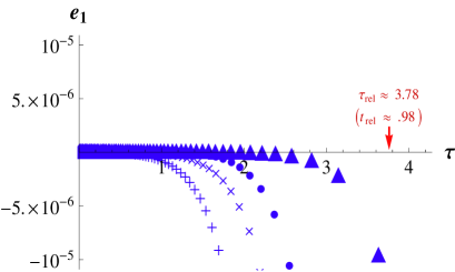
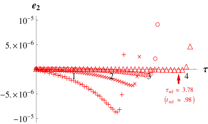
Figure 1: Colour online. Left panel: Resolution study of data from integration of inviscid Burgers equation. Plots, for different spatial resolutions, of the error $e_{1}$ with respect to the analytical solution. Symbols (blue online): ‘$+$’, ‘$\times$’, ‘$\bullet$’ and ‘$\blacktriangle$’ correspond respectively to resolutions 1024, 2048, 4096 and 16384. For reference, the reliability time computed from data of integration of mapped system at resolution 16384 is indicated by an arrow (orange online). Right panel: Resolution study of data from integration of regular mapped system. Plots, for different spatial resolutions, of the error $e_{2}$ with respect to the analytical solution. Symbols (red online): ‘$+$’, ‘$\times$’, ‘$\circ$’ and ‘$\triangle$’ correspond respectively to resolutions 1024, 2048, 4096 and 16384.

Notice that the scale used for both figures is the same. We observe that the convergence towards the analytical solution, as one increases the resolution, is much faster for the mapped system data than for the original inviscid Burgers system. Also, it is evident that the numerical simulation of the mapped system captures the singularity with better accuracy in the time domain for a given spatial resolution: figure 2, left panel, shows a comparison of $N=16384$ data from both methods. The error of the numerical data of the mapped system is one order of magnitude less than the error of the numerical data of the original system. This effect is due in part to the fact that the integration of the original inviscid Burgers system uses a constant timestep and therefore is bound to misrepresent the solution at times that are close to the singularity time $t_{\mathrm{end}}=1$. In contrast, the integration of the mapped system also uses a constant timestep but the singularity is at $\tau_{\mathrm{end}}=\infty\,,$ so the solution is well-resolved as long as the spatial resolution is not lost due to the localisation of the structures.

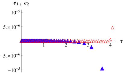
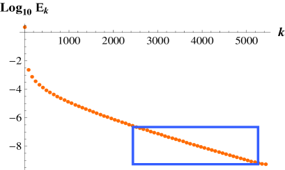
Figure 2: Colour online. Left Panel: Comparison of errors with respect to the analytical solution, of datasets obtained from integration of inviscid Burgers equation (error $e_{1}$, blue bullets) and regular mapped system (error $e_{2}$, red open circles), at fixed resolution 16384. Right panel: Log-lin plot of energy spectrum $E_{k}\propto|\hat{v}(k,t)|^{2}$ (orange bullets), of the solution $v(x,t)$ of the regular mapped equations at time $\tau=4.2,$ using data from numerical integration of regular mapped system. The resolution is 16384, corresponding to $k_{\max}=5461$ by the 2/3-rd dealiasing rule. It is possible to observe at least two decades of exponential decay of the spectrum (rectangular region, light blue online), in agreement with the criterion of reliability commonly used in the analiticity-strip method.

Finally, notice that for a given spatial resolution both original system and regular system have a ‘reliability time’ $\tau_{\mathrm{rel}}$ after which the fields are not well-resolved spatially anymore. One way to quantify the reliability time is by using the analiticity-strip method Sul83 , see also Bra83 ; BusKerr08 where the method is applied to 3D Euler equations. At resolution 16384, a calculation using the analiticity-strip method would give $\tau_{\mathrm{rel}}\approx 4.2,$ corresponding to original time $t_{\mathrm{rel}}\approx.99$ (see figure 2, right panel, and its caption). An ad-hoc and more conservative way to visualise the reliability time is to look at figure 1, right panel. The reliability time for a given spatial resolution is approximately the time when the local minimum of the error occurs. For example, at resolution 16384 the reliability time is $\tau_{\mathrm{rel}}\approx 3.78,$ corresponding to original time $t_{\mathrm{rel}}\approx 0.98\,.$ It is clear from figure 2, left panel, that the data from the mapped system agrees with the analytical solution up to times very close to the corresponding reliability time, while the data for inviscid Burgers system begins to diverge earlier.

As an extra check, using data from the numerical solution of the mapped regular system, we have confirmed the constancy of $K=\sigma(\tau)/\left(E_{\mathrm{map}}(\tau)\right)^{1/2}=\sigma_{0}/E^{1/2}=2\left(\pi/3\right)^{1/2}$ for all runs, within one part in $10^{-7}$ for resolution 1024, and well beyond the reliability time.

VI Conclusion and Discussion

We have established, for several equations of physical interest, a nonlinear time transformation and field rescaling that is based on a BKM-type of theorem, and which maps bijectively the original equations to a system that is globally regular in time.

We have learnt from the simple example of inviscid Burgers that the numerical integration of a mapped regular system produces more accurate and reliable results than the integration of the original system. The only way that the integration of the original system can match the regular system, is by upgrading the numerical method to an adaptive time stepping, based on the transformation (26), so that $d\tau=dt\times\|u_{x}(\cdot,t)\|_{\infty}$ is kept constant. In addition, we validated a procedure of spatial interpolation (of order 16) used to compute accurately the value of the supremum norm $\|v_{x}(\cdot,\tau)\|_{\infty}$. This procedure is essential for the numerical integration of the corresponding mapped regular system, not only in inviscid Burgers but also in 3D Euler, Navier Stokes and magnetohydrodynamics. It is worth mentioning that we also used this interpolation procedure to compute $\|u_{x}(\cdot,t)\|_{\infty}$ from the numerical data of inviscid Burgers equations. If we had just computed the collocation-point maximum value of the same quantity, we would have obtained a prohibitive amount of spurious oscillations (figure not shown).

In a forthcoming paper the method will be implemented to integrate the 3D Euler equations. We expect the integration of the regular mapped system to produce a significant improvement in accuracy. However in this case no analytical solution is at hand, so in order to draw robust conclusions on the trends we will need to make a late-time fit along with a careful determination of the reliability time. We are considering the possibility to include also a time-dependent spatial deformation in order to capture the localised structures as they develop. This procedure is in the spirit of McLau86 ; Land91 and the recent review Budd10 .

VII Acknowledgements

The author thanks E. Cox, F. Dias, D. D. Holm, R. M. Kerr, L. Ó Náraigh, R. Temam, E. S. Titi and an anonymous referee for useful comments. Support for this work was provided by UCD Seed Funding project SF304 and IRCSET Ulysses project “Singularities in three-dimensional Euler equations: simulations and geometry”.

References

-
[1]
http://www.claymath.org. - [2] V. I. Yudovich. Non-stationary flows of an ideal incompressible fluid. Z. Vyčisl. Mat. i Mat. Fiz., 3:1032–1066, 1963.
- [3] T. Kato. On classical solutions of the two-dimensional non-stationary Euler equation. Archive for Rational Mechanics and Analysis, 25:188–200, 1967.
- [4] O. A. Ladyženskaja. Unique global solvability of the three-dimensional Cauchy problem for the Navier-Stokes equations in the presence of axial symmetry. Zap. Naučn. Sem. Leningrad. Otdel. Mat. Inst. Steklov. (LOMI), 7:155–177, 1968.
- [5] M. R. Ukhovskii and V. I. Yudovich. Axially symmetric flows of ideal and viscous fluids filling the whole space. J. Appl. Math. Mech., 32:52–61, 1968.
- [6] A. Mahalov, E. S. Titi, and S. Leibovich. Invariant helical subspaces for the Navier-Stokes equations. Arch. Rational Mech. Anal., 112(3):193–222, 1990.
- [7] A. Dutrifoy. Existence globale en temps de solutions hélicoïdales des équations d’Euler. C. R. Acad. Sci. Paris Sér. I Math., 329(7):653 656, 1999.
- [8] B. Ettinger and E. S. Titi. Global existence and uniqueness of weak solutions of 3-D Euler equations with helical symmetry in the absence of vorticity stretching. SIAM J. Math. Anal., 41(1):269–296, 2009.
- [9] D. G. Ebin and J. Marsden. Groups of diffeomorphisms and the motion of an incompressible fluid. The Annals of Mathematics, Second Series, 92(1):102–163, 1970.
- [10] T. Kato. Nonstationary flows of viscous and ideal fluids in R3. J. Funct. Anal., 9:296–305, 1972.
- [11] J. P. Bourguignon and H. Brezis. Remarks on the Euler equation. Journal of functional analysis, 15(4):341–363, 1974.
- [12] R. Temam. On the Euler equations of incompressible perfect fluids. J. of Funct. Anal., 20:32–43, 1975.
- [13] J. T. Beale, T. Kato, and A. Majda. Remarks on the breakdown of smooth solutions for the 3-D Euler equations. Commun. Math. Phys., 94:61–66, March 1984.
- [14] G. Ponce. Remarks on a paper by J. T. Beale, T. Kato and A. Majda. Commun. Math. Phys., 98:349–353, 1985.
- [15] A. Ferrari. On the blow-up of solutions of the 3D Euler equations in a bounded domain. Commun. Math. Phys., 155:277–294, 1993.
- [16] P. Constantin. Geometric statistics in turbulence. SIAM Rev., 36:73–98, 1994.
- [17] P. Constantin, Ch. Fefferman, and A. J. Majda. Geometric constraints on potentially singular solutions for the 3D Euler equation. Commun. Partial Diff. Eqns., 21:559–571, 1996.
- [18] H. Kozono and Y. Taniuchi. Limiting case of the Sobolev inequality in BMO, with application to the Euler equations. Commun. Math. Phys., 214:191–200, 2000.
- [19] D. Cordoba and Ch. Fefferman. On the collapse of tubes carried by 3D incompressible flows. Commun. Math. Phys., 222:293–298, 2001.
- [20] J. Deng, T. Y. Hou, and X. Yu. Improved geometric condition for non-blowup of the 3D incompressible Euler equation. Commun. Partial Diff. Eqns., 31:293–306, 2003.
- [21] D. Chae. Remarks on the blow-up of the Euler equations and the related equations. Commun. Math. Phys., 245:539–550, 2003.
- [22] D. Chae. Local existence and blow-up criterion for the Euler equations in the Besov spaces. Asymptotic Analysis, 38:339–358, 2004.
- [23] D. Chae. Remarks on the blow-up criterion of the 3D Euler equations. Nonlinearity, 18:1021–1029, 2005.
- [24] J. Deng, T. Y. Hou, and X. Yu. Geometric properties and non-blowup of 3D incompressible Euler flow. Commun. Partial Diff. Eqns., 30:225–243, 2005.
- [25] J. Deng, T. Y. Hou, and X. Yu. A level set formulation for the 3D incompressible Euler equations. Methods Appl. Anal., 12:427–440, 2005.
- [26] D. Chae. On the finite-time singularities of the 3D incompressible Euler equations. Commun. Pure Appl. Math., 60(4):597–617, 2007.
- [27] J. D. Gibbon. Ortho-normal quaternion frames, Lagrangian evolution equations and the three-dimensional Euler equations. Russ. Math. Surv., 62:1–26, 2007.
- [28] J. D. Gibbon, M. D. Bustamante, and R. M. Kerr. The three-dimensional Euler equations: singular or non-singular? Nonlinearity, 21:T123, 2008.
- [29] C. Bardos, S. Benachour, and M. Zerner. Analyticité des solutions périodiques de l’équation d’Euler en deux dimensions. C. R. Acad. Sci. Paris, 282A:995–998, 1976.
- [30] R. H. Morf, S. A. Orszag, and U. Frisch. Spontaneous singularity in three-dimensional, inviscid incompressible flow. Phys. Rev. Lett., 44:572–575, 1980.
- [31] A. J. Chorin. The evolution of a turbulent vortex. Commun. Math. Phys., 83:517–535, 1982.
- [32] M. E. Brachet, D. I. Meiron, S. A. Orszag, B. G. Nickel, R. H. Morf, and U. Frisch. Small-scale structure of the Taylor-Green vortex. J. Fluid Mech., 130:411–452, 1983.
- [33] E. D. Siggia. Collapse and amplification of a vortex filament. Phys. Fluids, 28:794–805, 1984.
- [34] S. Kida. Three-dimensional periodic flows with high symmetry. J. Phys. Soc. Japan, 54:2132–2136, 1985.
- [35] A. Pumir and R. M. Kerr. Numerical simulation of interacting vortex tubes. Phys. Rev. Lett., 58:1636–1639, 1987.
- [36] W. Ashurst and D. Meiron. Numerical study of vortex reconnection. Phys. Rev. Lett., 58:1632–1635, 1987.
- [37] A. Pumir and E. D. Siggia. Collapsing solutions to the 3D Euler equations. Phys. Fluids A, 2:220–241, 1990.
- [38] J. B. Bell and D. L. Marcus. Vorticity intensification and transition to turbulence in the three-dimensional Euler equations. Commun. Math. Phys., 147:371–394, 1992.
- [39] M. E. Brachet, V. Meneguzzi, A. Vincent, H. Politano, and P.-L. Sulem. Numerical evidence of smooth selfsimilar dynamics and the possibility of subsequent collapse for ideal flows. Phys. Fluids A, 4:2845–2854, 1992.
- [40] R. M. Kerr. Evidence for a singularity of the three-dimensional incompressible Euler equations. Phys. Fluids A, 5:1725–1746, 1993.
- [41] O. N. Boratav and R. B. Pelz. Direct numerical simulation of transition to turbulence from a high-symmetry initial condition. Phys. Fluids, 6:2757–2784, 1994.
- [42] R. B. Pelz and Y. Gulak. Evidence for a real-time singularity in hydrodynamics from time series analysis. Phys. Rev. Lett., 79:4998 5001, 1997.
- [43] R. Grauer, C. Marliani, and K. Germaschewski. Adaptive mesh refinement for singular solutions of the incompressible Euler equations. Phys. Rev. Lett., 80:4177–4180, 1998.
- [44] R. B. Pelz. Symmetry and the hydrodynamic blow-up problem. J. Fluid Mech., 444:299–320, 2001.
- [45] R. M. Kerr. Vortex collapse and turbulence. Fluid Dyn. Res., 36:249–260, 2005.
- [46] R. B. Pelz and K. Ohkitani. Linearly strained flows with and without boundaries–the regularizing effect of the pressure term. Fluid Dyn. Res., 36:193–210, 2005.
- [47] Y. Gulak and R. B. Pelz. High-symmetry Kida flow: time series analysis and resummation. Fluid Dyn. Res., 36:211 220, 2005.
- [48] C. Cichowlas and M. E. Brachet. Evolution of complex singularities in Kida-Pelz and Taylor-Green inviscid flows. Fluid Dyn. Res., 36:239 248, 2005.
- [49] R. M. Kerr. Vorticity and scaling of collapsing Euler vortices. Phys. Fluids A, 17:075103–075114, 2005.
- [50] W. Pauls, T. Matsumoto, U. Frisch, and J. Bec. Nature of complex singularities for the 2D Euler equation. Physica D, 219:40–59, 2006.
- [51] T. Y. Hou and R. Li. Dynamic Depletion of Vortex Stretching and Non-Blowup of the 3-D Incompressible Euler Equations. J. Nonlinear Sci., 16:639–664, 2006.
- [52] P. Orlandi and G. Carnevale. Nonlinear amplification of vorticity in inviscid interaction of orthogonal Lamb dipoles. Phys. Fluids, 19:057106, 2007.
- [53] T. Grafke, H. Homann, J. Dreher, and R. Grauer. Numerical simulations of possible finite time singularities in the incompressible Euler equations: comparison of numerical methods. Physica D: Nonlinear Phenomena, 237:1932–1936, 2008.
- [54] T. Y. Hou and R. Li. Blowup or no blowup? The interplay between theory and numerics. Physica D: Nonlinear Phenomena, 237:1937–1944, 2008.
- [55] M. D. Bustamante and R. M. Kerr. 3D Euler about a 2D symmetry plane. Physica D: Nonlinear Phenomena, 237:1912–1920, 2008.
- [56] C. Sulem, P. L. Sulem, and H. Frisch. Tracing complex singularities with spectral methods. Journal of Computational Physics, 50:138–161, 1983.
- [57] R. E. Caflisch, I. Klapper, and G. Steele. Remarks on singularities, dimension and energy dissipation for ideal hydrodynamics and MHD. Communications in Mathematical Physics, 184:443–455, 1997.
- [58] S. D. Poisson. Mémoire sur la théorie du son. Journal de l’Ecole Polytechnique, 14 éme cahier, 7:319–392, 1808.
- [59] D. W. McLaughlin, G. C. Papanicolaou, C. Sulem, and P. L. Sulem. Focusing singularity of the cubic Schrödinger equation. Phys. Rev. A, 34:1200–1210, 1986.
- [60] M. J. Landman, G. C. Papanicolaou, C. Sulem, P. L. Sulem, and X. P. Wang. Stability of isotropic singularities for the nonlinear Schrödinger equation. Physica D, 47:393–415, 1991.
- [61] C. J. Budd and J. F. Williams. How to adaptively resolve evolutionary singularities in differential equations with symmetry. J. Eng. Math., 66:217–236, 2010.