On Taming the Warped Radion with Supersymmetry

Abstract

In warped models that solve the hierarchy problem, there is generally no dynamical relation between the size of the fifth dimension and the scale of electroweak symmetry breaking (EWSB). The establishment of such a relation, without fine-tuning, requires that Casimir contributions to the radion potential not exceed the energy density associated with EWSB. Here, we examine the use of supersymmetry for controlling the Casimir energy density and making quantum contributions calculable. We compute the effects of supersymmetry breaking at the UV and IR boundaries of warped backgrounds, in the presence of brane localized kinetic terms. Various limits of supersymmetry breaking are examined. We find that when supersymmetry is broken on the UV brane, vacuum contributions to the radion potential can be controlled (as likely necessary for EWSB to govern the radion potential) via small soft masses as well as a “double volume suppression.” Our formalism can also provide a setup for radion stabilization by bulk fields, when supersymmetry is broken on both the UV and the IR branes.

1 Introduction

An interesting resolution of the gauge hierarchy problem is offered by warped models based on the original Randall-Sundrum (RS) geometry [1] which is a slice of the 5D Anti de Sitter (AdS₅) spacetime. This geometry, characterized by a curvature scale $k$, is bounded by flat walls, often referred to as the UV and IR branes. In these models the fundamental 5D scales of the theory, perhaps near the 4D Planck scale $M_{P}\sim 10^{19}$ GeV, redshift to the weak scale of order 1 TeV as one goes from the UV brane to the IR brane. The redshift is caused by an exponential warp factor and a Planck-weak hierarchy of order $10^{16}$ can be achieved if the size $L$ of the extra dimension satisfies $kL\gtrsim 30$. In addition, placing the Standard Model (SM) gauge [2, 3] and fermion [4] content in all 5D can yield a realistic explanation of 4D flavor [5], where heavy fermions are localized towards the source of the electroweak symmetry breaking (EWSB) on the IR brane, while light fermions are UV-brane localized, so that their small masses arise from an exponentially small wavefunction overlap with the IR brane.

While many features of the SM can be accommodated and explained in warped scenarios, quite often the scale $m_{W}\sim 10^{2}$ GeV of EWSB is simply assumed to be set by the IR-brane physical scale $\tilde{k}\equiv k\,e^{-kL}$. Since various bounds from precision and collider phenomenology favor $\tilde{k}\gtrsim 1$ TeV, this often reintroduces some level of fine-tuning into the models. It would then be interesting to find a dynamical mechanism whereby EWSB sets $kL$ near the requisite value, and that naturally leads to a separation between $m_{W}$ and $\tilde{k}$. As the size of the extra dimension is controlled by the dynamics of the radion scalar, one would like to generate an appropriate potential for the radion through EWSB.

In fact, such a model was proposed in Ref. [6], where the condensation of IR-localized top quarks of the SM is triggered by strong interactions mediated by Kaluza-Klein (KK) gluons. This condensation breaks the electroweak symmetry and through its radion-dependence can also stabilize the size of the fifth dimension. In this top-condensation scenario, the IR-bane scale is set by $\tilde{k}\sim 10$ TeV, which has the added benefit of avoiding most severe constraints on warped models, while providing a GeV-scale radion as its low energy signature [6, 7]. Due to the dynamical nature of the condensation, the separation between the IR-brane scale and the weak scale is natural. However, one has to assume that other contributions to the radion potential would not overwhelm the electroweak contribution. In particular, one may naively expect that the corrections from zero-point energies of bulk fields to the radion potential (which contain the calculable Casimir energy) are of order $\tilde{\Lambda}^{4}/(16\pi^{2})$, where the effective theory cutoff-scale $\tilde{\Lambda}\sim 4\pi\tilde{k}$.

Given the above situation, either one has to resort to a severe fine-tuning, or else find a way to suppress such cutoff scale effects. In this work, we adopt the second possibility and examine how supersymmetry (SUSY) can be used to protect the radion potential from too large cutoff dominated contributions. Since in the limit of exact SUSY all vacuum energies cancel out, in supersymmetric scenarios the full radion potential is expected to be far less sensitive to the cutoff. We will consider soft supersymmetry breaking by localized mass terms on both the UV and the IR branes. In addition, we allow for the presence of brane kinetic terms (BKTs), which are expected to be induced radiatively, and that are known to have a strong effect on the KK spectrum [8, 9, 10]. We find that when SUSY is broken on the UV brane, this vacuum energy contribution is of order $\tilde{k}^{2}m_{\lambda}^{2}/(16\pi^{2}kL)$, where $m_{\lambda}$ is the physical mass of the (would-be zero-mode) gaugino. Hence, there is a suppression from the dependence on soft masses, as well as an additional volume-suppression. This result suggests that a supersymmetric version of the scenario presented in Ref. [6] may be realizable without the need for fine-tuning. Even though dynamical EWSB scenarios, which will be pursued in Ref. [11], provide our basic motivation for this study, we will also consider the effect of a supersymmetric bulk in other contexts. In particular, in models where the Casimir energy is responsible for generating the radion potential [12, 13, 14, 15], the success of the mechanism depends on the size and sign of certain contributions that are in general not calculable. We show how a supersymmetric framework with SUSY broken at a high scale may realize the radion stabilization mechanism by gauge fields proposed in Ref. [14]. The above radion stabilization mechanisms are distinct from stabilization by bulk fields that acquire vacuum expectation values (VEV’s) at tree level, as in Ref. [16]. Related work has appeared in Refs. [17, 18, 19].

The structure of this paper is as follows. In the next section, we consider the case of a bulk scalar field, with brane localized masses and kinetic terms, and evaluate the radion potential generated by the Casimir effect from the scalar. The results are sufficiently general to be applied to fields of arbitrary spin that obey arbitrary boundary conditions. We provide such a generalization to particles of different spin in Section 3. We apply our results to study scenarios in which supersymmetry is broken on the UV or IR branes, as may be relevant in different models, in Sections 4. We present our conclusions in Section 5, followed by Appendices A (conventions for KK reduction) and B (approximate expressions for the radion potential in various limits).

2 Radion Potential from Scalar Fields

In this section, we summarize the results for the radion potential at one-loop order in warped backgrounds. Since this potential arises through the radion-dependence of the KK masses associated with bulk fields propagating in compact dimensions, we focus on describing the spectrum of such fields. The spectrum depends on the quadratic terms in the action (including both bulk and brane-localized operators), as well as on the boundary conditions. Since the results for fields in different spin representations of the Lorentz group can be expressed in terms of those of a scalar field, we start with the real scalar case. For reference, further details regarding the boundary conditions, the KK decomposition, orthonormality relations, etc. are relegated to Appendix A.

2.1 Bulk Fields with Brane-Localized Terms

We consider a slice of AdS₅:

$$ds^{2}=e^{-2ky}\eta_{\mu\nu}dx^{\mu}dx^{\nu}-dy^{2}\leavevmode\nobreak\ ,$$ (1)

where $k$ is the AdS curvature and $y\in[0,L]$ parametrizes the fifth dimension. The action for a free real scalar field is

$$S=\int\!d^{4}x\int_{0}^{L}\!dy\,\sqrt{g}\left\{\frac{1}{2}g^{MN}\partial_{M}\Phi\partial_{N}\Phi-\frac{1}{2}M^{2}\Phi^{2}+2\delta(y){\cal L}_{0}+2\delta(y-L){\cal L}_{L}\right\}\leavevmode\nobreak\ ,$$ (2)

where the brane-localized terms are given by 

$${\cal L}_{0} = \frac{1}{2}r_{UV}\,g^{\mu\nu}\partial_{\mu}\Phi\partial_{\nu}\Phi-\frac{1}{2}M_{0}\Phi^{2}\leavevmode\nobreak\ ,$$ (3)

$${\cal L}_{L} = \frac{1}{2}r_{IR}\,g^{\mu\nu}\partial_{\mu}\Phi\partial_{\nu}\Phi-\frac{1}{2}M_{L}\Phi^{2}\leavevmode\nobreak\ .$$ (4)

The kinetic coefficients $r_{UV}$ and $r_{IR}$ have mass dimension $-1$, while $M_{0}$ and $M_{L}$ have mass dimension $1$. It is convenient to introduce a dimensionless parameter $\alpha$ (that we will call the “index” of the field) and new mass parameters $m_{UV}$ and $m_{IR}$ by writing the bulk and localized masses as

$$M^{2} = \left(\alpha^{2}-4\right)k^{2}\leavevmode\nobreak\ ,$$ (5)

$$M_{0} = -\left(\alpha-2\right)k+m_{UV}\leavevmode\nobreak\ ,\hskip 28.45274ptM_{L}\leavevmode\nobreak\ =\leavevmode\nobreak\ \left(\alpha-2\right)k+m_{IR}\leavevmode\nobreak\ .$$ (6)

Performing the KK decomposition in the usual manner (see Appendix A), one finds that the KK spectrum, $m_{n}$, is determined by 

$$F(m_{n}/k)\equiv\tilde{J}^{IR}_{\alpha}\!\left(\frac{m_{n}}{k}e^{kL}\right)\tilde{Y}^{UV}_{\alpha}\!\left(\frac{m_{n}}{k}\right)-\tilde{J}^{UV}_{\alpha}\!\left(\frac{m_{n}}{k}\right)\tilde{Y}^{IR}_{\alpha}\!\left(\frac{m_{n}}{k}e^{kL}\right) = 0\leavevmode\nobreak\ ,$$ (7)

where $L$ is the radion VEV. Here, we have introduced the functions

$$\tilde{J}^{UV}_{\alpha}(z) = zJ_{\alpha-1}(z)+b_{UV}(z)J_{\alpha}(z)\leavevmode\nobreak\ ,$$ (8)

$$\tilde{J}^{IR}_{\alpha}(z) = zJ_{\alpha-1}(z)-b_{IR}(z)J_{\alpha}(z)\leavevmode\nobreak\ ,$$ (9)

with analogous expressions for $\tilde{Y}^{UV}_{\alpha}(z)$ and $\tilde{Y}^{IR}_{\alpha}(z)$, and defined

$$b_{i}(z) = \hat{r}_{i}z^{2}-\hat{m}_{i}\leavevmode\nobreak\ ,\hskip 28.45274pti=UV,IR$$ (10)

by using the dimensionless parameters $\hat{m}_{i}=m_{i}/k$, $\hat{r}_{i}=k\,r_{i}$.

For $\hat{m}_{UV}=\hat{m}_{IR}=0$ (the SUSY limit) there is a scalar zero-mode with an exponential profile controlled by the dimensionless parameter $\alpha$ (see Appendix A.2 for details). This profile coincides with that of a 5D fermion with a bulk Dirac mass term written as $M=ck$, where $\alpha=c+\frac{1}{2}$ [4]. We will refer to fields with $\alpha<1$ as “IR localized fields”, those with $\alpha=1$ as “flat fields” and those with $\alpha>1$ as “UV localized fields”. When $\hat{m}_{UV}$ and/or $\hat{m}_{IR}$ deviate from zero, the scalar zero-mode is lifted: for positive $\hat{m}_{UV,IR}$ it becomes massive, while for negative $\hat{m}_{UV,IR}$ a tachyonic mode appears. Note also that one can interpolate between Neumann-type boundary conditions (setting $m_{i}=0$) and Dirichlet boundary conditions ($m_{i}\to\infty$) on the $i^{\rm th}$ ($=UV$ or $IR$) brane, and therefore our results are sufficiently general to capture the dependence of the radion potential on the choice of boundary conditions for the bulk field.

It is also worth pointing out that, when $\hat{r}_{i}=\hat{m}_{i}=0$, the massive KK spectrum is identical for fields with index $\alpha=1+\delta\alpha$ and fields with index $\alpha=1-\delta\alpha$, for any $\delta\alpha$, as can be easily checked from Eq. (7). However, non-vanishing $\hat{r}_{i}$ and/or $\hat{m}_{i}$ introduce a distinction between the KK spectra of UV versus IR localized fields.

2.2 One-Loop Effective Potential

The presence of fields propagating in a $D$-dimensional spacetime with $D-4$ compact dimensions generically leads to a vacuum energy that depends on the overall volume of the extra dimensions as well as on the various shape moduli. For a single compact extra dimension one simply gets a potential for its size $L$, given at one-loop order by

$$V_{\rm eff}(L) = \frac{1}{2}\sum_{n}\int\!\frac{d^{4}p_{E}}{(2\pi)^{4}}\,\ln\left(\frac{p^{2}_{E}+m^{2}_{n}}{\mu^{2}}\right)\leavevmode\nobreak\ ,$$ (11)

where the radion dependence enters through the spectrum, $m_{n}(L)$. Here the integration is over Euclidean momentum and $\mu$ is the renormalization scale. Eq. (11) is the contribution due to a bulk real scalar, but we will consider other types of fields in Section 3. In this work, we will assume that the backreaction due to the one-loop vacuum energy is small, so that the AdS₅ metric of Eq. (1) gives a good approximation. The effective potential contains divergent pieces that correspond to a renormalization of the 5D cosmological constant, as well as of the IR and UV brane tensions. The first two lead to radion-dependent terms that behave like $e^{-4kL}$. Additionally, there are calculable terms, usually referred to as the Casimir energy, that can have a more complicated radion dependence and can sometimes stabilize the distance between the branes [14]. In order to exhibit the various radion-dependent contributions, one can evaluate Eq. (11) using standard methods based on $\zeta$-function regularization. The regularized radion potential has been computed in Refs. [12, 13, 14, 15], and takes the form

$$V_{\rm eff}(L) = \frac{k^{4}}{16\pi^{2}}\left[{\cal I}_{UV}+e^{-4kL}{\cal I}_{IR}\right]+V_{\rm Casimir}(L)\leavevmode\nobreak\ ,$$ (12)

where the “Casimir energy” is given by 

$$V_{\rm Casimir}(L) = \frac{k^{4}e^{-4kL}}{16\pi^{2}}\int_{0}^{\infty}\!dt\,t^{3}\ln\left|1-\frac{\tilde{K}^{IR}_{\alpha}(t)}{\tilde{I}^{IR}_{\alpha}(t)}\frac{\tilde{I}^{UV}_{\alpha}(te^{-kL})}{\tilde{K}^{UV}_{\alpha}(te^{-kL})}\right|\leavevmode\nobreak\ ,$$ (13)

and the “generalized” Bessel functions are defined by

$$\tilde{K}^{UV}_{\alpha}(z) = zK_{\alpha-1}(z)-\tilde{b}_{UV}(z)K_{\alpha}(z)\leavevmode\nobreak\ ,$$ (14)

$$\tilde{I}^{UV}_{\alpha}(z) = zI_{\alpha-1}(z)+\tilde{b}_{UV}(z)I_{\alpha}(z)\leavevmode\nobreak\ ,$$ (15)

$$\tilde{K}^{IR}_{\alpha}(z) = zK_{\alpha-1}(z)+\tilde{b}_{IR}(z)K_{\alpha}(z)\leavevmode\nobreak\ ,$$ (16)

$$\tilde{I}^{IR}_{\alpha}(z) = zI_{\alpha-1}(z)-\tilde{b}_{IR}(z)I_{\alpha}(z)\leavevmode\nobreak\ .$$ (17)

Here, $\tilde{b}_{i}(z)\equiv-\hat{r}_{i}z^{2}-\hat{m}_{i}$ has an additional minus sign in the first term compared to Eq. (10) as a result of the Wick rotation involved in obtaining Eq. (12).

The terms proportional to ${\cal I}_{UV}$ and ${\cal I}_{IR}$ in Eq. (12) correspond to UV and IR brane tension renormalizations, respectively. (${\cal I}_{UV}$ depends only on the UV quantities $\hat{m}_{UV}$ and $\hat{r}_{UV}$, while ${\cal I}_{IR}$ depends only on the IR quantities $\hat{m}_{IR}$ and $\hat{r}_{IR}$.) Such contributions are in general uninteresting, since there are additional incalculable (and most likely larger) contributions that renormalize the brane tensions. Hence, we will focus on the Casimir term in what follows.

2.3 The Casimir Energy

The Casimir energy contribution to the radion potential, Eq. (13), which contains the 5D non-local, and therefore calculable, terms has been computed in the literature [12, 13, 14]. Although the expression given in Eq. (13) can be easily evaluated numerically for any value of $L$, and for fixed values of the parameters in the Lagrangian: $\alpha=c+1/2$, $m_{i}$ and $r_{i}$ ($i=UV$ or $IR$), it is useful to have analytic approximations that make the radion dependence more explicit. We derive general expressions for the case that $e^{-kL}\ll 1$ in Appendix B. These result from the fact that the radion dependence is fully contained in the “UV factor” $\tilde{I}^{UV}_{\alpha}(te^{-kL})/\tilde{K}^{UV}_{\alpha}(te^{-kL})$, which can legitimately be approximated by a small argument expansion of the Bessel functions. Thus, the functional dependence of the Casimir energy on $L$ is determined by the UV quantities. In particular, one finds that $\hat{m}_{UV}$ defines a characteristic scale $L_{T}$ according to 

$$\begin{array}[]{lcl}e^{2kL_{\rm T}}\hat{m}_{UV}=1\leavevmode\nobreak\ ,&&\textrm{for }\alpha\geq 1\leavevmode\nobreak\ ,\\[1.99997pt] &\textrm{or}&\\[1.99997pt] e^{2\alpha kL_{\rm T}}\hat{m}_{UV}=1\leavevmode\nobreak\ ,&&\textrm{for }\alpha<1\leavevmode\nobreak\ .\end{array}$$ (21)

As shown in Appendix A.2, the above transition signals whether a KK state parametrically lighter than the KK scale, $k\,e^{-kL}$, exists or not. For $L\gg L_{T}$ (“large $m_{UV}$”) and $\alpha>0$, one finds

$$V_{\rm Casimir} \approx \frac{k^{4}e^{-2(2+\alpha)kL}}{16\pi^{2}}\frac{2^{1-2\alpha}(\hat{m}_{UV}-2\alpha)}{\hat{m}_{UV}\Gamma(\alpha)\Gamma(\alpha+1)}\int_{0}^{\infty}\!dt\,t^{3+2\alpha}\frac{\tilde{K}^{IR}_{\alpha}(t)}{\tilde{I}^{IR}_{\alpha}(t)}\leavevmode\nobreak\ ,$$ (22)

while the expressions for $\alpha=0$ and $\alpha<0$ are given in Eqs. (72) and (73) of Appendix B, respectively. For $L\ll L_{T}$ (“small $m_{UV}$”), which is the case with a light would-be zero mode in the spectrum, but $kL\gg 1$, one has to distinguish several cases. For instance, for moderate localization of this mode near the IR brane, one finds

$$V_{\rm Casimir} \approx \frac{k^{4}e^{-4kL}}{16\pi^{2}}\int_{0}^{\infty}\!dt\,t^{3}\ln\left|1-\frac{2\sin(\pi\alpha)}{\pi}\,\frac{\tilde{K}^{IR}_{\alpha}(t)}{\tilde{I}^{IR}_{\alpha}(t)}\right|\leavevmode\nobreak\ ,\hskip 28.45274pt\textrm{for }0<\alpha<1\leavevmode\nobreak\ .$$ (23)

For the flat case, $\alpha=1$:

$$V_{\rm Casimir} \approx -\frac{k^{4}e^{-4kL}}{16\pi^{2}}\,\frac{1}{kL+\hat{r}_{UV}}\int_{0}^{\infty}\!dt\,t^{3}\frac{\tilde{K}^{IR}_{\alpha=1}(t)}{\tilde{I}^{IR}_{\alpha=1}(t)}\leavevmode\nobreak\ ,$$ (24)

where, for simplicity, we have ignored the numerically small Euler constant, as well as a $\ln(t/2)$ term that makes a relatively small difference [see third line in Eq. (79) of Appendix B]. Finally, for moderate localization near the UV brane one finds

$$V_{\rm Casimir} \approx -\frac{k^{4}e^{-2(\alpha+1)kL}}{16\pi^{2}}\,\frac{2^{3-2\alpha}}{\Gamma(\alpha)\left[\Gamma(\alpha-1)+2\hat{r}_{UV}\Gamma(\alpha)\right]}\int_{0}^{\infty}\!dt\,t^{1+2\alpha}\frac{\tilde{K}^{IR}_{\alpha}(t)}{\tilde{I}^{IR}_{\alpha}(t)}\leavevmode\nobreak\ ,\hskip 14.22636pt\textrm{for }1<\alpha<2\leavevmode\nobreak\ .$$

The case of more extreme IR localization (with $\alpha\leq 0$) is given in Eq. (73), while for more extreme UV localization (with $\alpha\geq 2$) the result can be easily obtained from Eq. (79) of Appendix B. In Eqs. (23), (24) and (LABEL:VCasSmallmUV1alpha2), we have ignored terms subleading in $\hat{m}_{UV}$. In SUSY theories that are softly broken by UV brane localized masses, the above leading contributions cancel out within a given supermultiplet, and one should keep the terms subleading in $\hat{m}_{UV}$. We postpone such an application to Section 4. For the time being we simply make a few observations that follow from the previous results. First, when $\hat{m}_{UV}$ is large in the sense defined above, the Casimir energy is suppressed by a factor $e^{-2\alpha kL}$ on top of the naive $e^{-4kL}$ expected from the scaling of the KK masses. This happens for any $\alpha>0$ [see Eq. (22)]. Second, for small $\hat{m}_{UV}$, fields localized near the IR brane give a radion dependence identical to the one arising from an IR brane tension, up to exponentially small terms [see Eq. (23)]. Third, as pointed out in Ref. [14], flat fields produce only a volume suppression [see Eq. (24)] that allows their contribution to be plausibly comparable to the IR brane tension contribution, and in certain cases can lead to radion stabilization. And finally, fields localized towards the UV brane give a contribution that is exponentially small compared to that of the IR brane tension [see Eq. (LABEL:VCasSmallmUV1alpha2)].

In applications, one often finds fields obeying Dirichlet boundary conditions on both branes. The contribution to the Casimir energy from such fields can be easily obtained by taking the limits $\hat{m}_{UV}\to\infty$ and $\hat{m}_{IR}\to\infty$ [e.g. in Eq. (22)]. For the Casimir energy part, one finds that for $\alpha>0$:

$$V^{(-,-)}_{\rm Casimir} \approx \frac{B^{(-,-)}_{IR}k^{4}}{16\pi^{2}}\,e^{-2(2+\alpha)kL}\leavevmode\nobreak\ ,$$ (26)

where

$$B^{(-,-)}_{IR} = -\frac{2^{1-2\alpha}}{\Gamma(\alpha)\Gamma(\alpha+1)}\int_{0}^{\infty}\!dt\,t^{3+2\alpha}\frac{K_{\alpha}(t)}{I_{\alpha}(t)}\leavevmode\nobreak\$$ (27)

depends only on the localization of the field. We plot $B^{(-,-)}_{IR}$ in Fig. 1, which shows that it is always negative. Eq. (26) shows that these effects are exponentially suppressed compared to the IR brane tension contribution. The exception occurs for $\alpha\approx 0$, in which case one should use [see Eq. (72) of Appendix B]

$$B^{(-,-)}_{IR} \approx -\frac{1}{kL}\int_{0}^{\infty}\!dt\,t^{3}\frac{K_{\alpha=0}(t)}{I_{\alpha=0}(t)}\leavevmode\nobreak\ ,$$ (28)

instead of Eq. (27), setting $\alpha=0$ in Eq. (26).

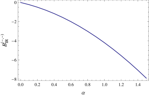
Figure 1: $B^{(-,-)}_{IR}$ of Eq. (27) as a function of $\alpha$. This determines the contribution to the effective potential due to fields obeying $(-,-)$ boundary conditions according to Eq. (26). At very small $\alpha$ one should use Eq. (28), but this detail is imperceptible in the figure when $kL\gg 1$ since $B^{(-,-)}_{IR}$ is very small.

For $\alpha<0$, one finds [see Eq. (73) of Appendix B, with $\hat{m}_{IR}\to\infty$]:

$$V^{(-,-)}_{\rm Casimir} \approx \frac{k^{4}e^{-4kL}}{16\pi^{2}}\int_{0}^{\infty}\!dt\,t^{3}\ln\left|1+\frac{2\sin(\pi\alpha)}{\pi}\,\frac{K_{\alpha}(t)}{I_{\alpha}(t)}\right|\leavevmode\nobreak\ .$$ (29)

In fact, in the case of vanishing BKT’s, the $(-,-)$ contribution of a field with index $\alpha$ is identical to that of a field with vanishing localized masses and index $\alpha+1$ (see Section 3). The results of this section will be used in Sections 3 and 4.

3 Higher Spins and SUSY Multiplets

In this section we give a brief summary of the contributions to the radion potential from 5D fields of spin-$1/2$, $1$, $3/2$ and $2$, and then give the results for the net effective potential from various SUSY multiplets. In general, these contributions can be simply expressed in terms of the effective potential due to a real scalar field, which was evaluated above. One finds

$$V_{\rm eff}^{s\geq 0}(L) = (-1)^{2s}\,n\,V^{\textrm{Real scalar}}_{\rm eff}(L)\leavevmode\nobreak\ ,$$ (30)

where $V^{\textrm{Real scalar}}_{\rm eff}(L)=V_{\rm eff}(L)$ is given in Eq. (12) and $n$ is the number of physical degrees of freedom of a massive 4D field of spin $s$ (taking into account whether the field is real or complex, in the bosonic case). Deriving the result above is straightforward for complex scalars or fermions, but requires adding a gauge-fixing term to the action for higher spins. One also has to include the associated Faddeev-Popov determinant, which simply cancels the spurious contributions to the potential from the gauge degrees of freedom. Here we just use Eq. (30) in our applications below (with $n=2$ for complex scalars, $n=4$ for fermions, $n=3$ for (real) gauge bosons, $n=5$ for the graviton and $n=8$ for the gravitino). Based on this, we can put together the total contributions to the radion potential due to (softly broken) SUSY multiplets. Since the compactification breaks the 5D $N=1$ SUSY (4D $N=2$) down to 4D $N=1$ SUSY, it is useful to classify the field content in 4D $N=1$ language.

Starting with hypermultiplets, and listing only the on-shell fields, these consist of two 4D $N=1$ chiral multiplets: $(\Phi_{1},\psi_{1})$ and $(\Phi_{2},\psi_{2})$. If the pair $(\Phi_{1},\psi_{1})$ has “localization parameter” (or index) $\alpha$, then the second pair of fields, $(\Phi_{2},\psi_{2})$, has index $\alpha-1$. Both $\Phi_{2}$ and $\psi_{2}$ obey Dirichlet boundary conditions, so that they do not have zero-modes. For vanishing kinetic terms, $\hat{r}_{UV}=\hat{r}_{IR}=0$, and arbitrary UV and/or IR localized masses for the complex scalar $\Phi_{1}$ (recall that $\Phi_{2}$ vanishes on the branes) the effective potential is:

$$\left.\rule{0.0pt}{14.22636pt}V^{\rm Hyper}_{\rm eff}\right|_{\hat{r}_{i}=0} = 2\times\left.\rule{0.0pt}{14.22636pt}V_{\rm eff}(L)\right|_{\alpha;\hat{r}_{i}=0;\hat{m}_{i}}+2\times\left.V^{(-,-)}_{\rm eff}(L)\right|_{\alpha-1}-4\times\left.\rule{0.0pt}{14.22636pt}V_{\rm eff}(L)\right|_{\alpha;\hat{r}_{i}=0;\hat{m}_{i}=0}\leavevmode\nobreak\ ,$$ (31)

where $V_{\rm eff}(L)$ is given in Eq. (12), and $V^{(-,-)}_{\rm eff}(L)$, which depends only on the index $\alpha$, is the effective potential for a real scalar obeying Dirichlet boundary conditions on both branes [the (approximate) Casimir energy part is given in Eqs. (27), (28) or (29), according to the value of $\alpha$]. We have also indicated the index $\alpha$ of the “generalized” Bessel functions [see Eq. (14)-(17)] to be used in each term. The fermions $\psi_{1}$ and $\psi_{2}$ contribute together as a KK tower of Dirac fermions through the last term in Eq. (31). The total effective potential above vanishes in the SUSY limit, i.e. when $\hat{m}_{i}=0$. Indeed, in this case the approximate expressions (23), (24) or (LABEL:VCasSmallmUV1alpha2) for $V_{\rm Casimir}$ hold, depending on the value of $\alpha$, and one can explicitly see that the Casimir energy contributions from the components of the hypermultiplet cancel out. More generally, the exact cancellations follow from

$$\left.\frac{\tilde{K}^{i}_{\alpha}(z)}{\tilde{I}^{i}_{\alpha}(z)}\right|_{\hat{r}_{i}=0;\hat{m}_{i}=0} = \left.\frac{\tilde{K}^{i}_{\alpha-1}(z)}{\tilde{I}^{i}_{\alpha-1}(z)}\right|_{\hat{r}_{i}=0;\hat{m}_{i}=\infty}\leavevmode\nobreak\ ,\hskip 42.67912pt\textrm{for}\leavevmode\nobreak\ i=UV,IR\leavevmode\nobreak\ ,$$ (32)

which implies that the Casimir energies, Eq. (13), are the same for a field with index $\alpha-1$ that obeys Dirichlet boundary conditions (obtained by taking $\hat{m}_{i}\to\infty$), and for a field with $\hat{m}_{i}=0$ and index $\alpha$ (i.e. the KK spectra are identical in these two cases).

When the brane kinetic terms are non-zero one has to be more careful, since supersymmetry requires that the action for the “odd” scalar field, $\Phi_{2}$, contain special singular terms on the branes. These can be derived by writing the SUSY action in 4D $N=1$ language, following the formalism of Refs. [21, 22], together with brane-localized minimal Kähler terms for the “even” chiral superfield, $(\Phi_{1},\psi_{1})$, and then integrating out the auxiliary fields. Besides brane localized terms (with $\partial_{\mu}$ derivatives) for $\Phi_{1}$ and $\psi_{1}$, one finds that the bulk kinetic term for $\Phi_{2}$ should be replaced by

$$|\partial_{M}\Phi_{2}|^{2}\to|\partial_{\mu}\Phi_{2}|^{2}-\frac{1}{1+\sum_{i=UV,IR}r_{i}\delta(y-y_{i})}|\partial_{5}\Phi_{2}|^{2}\leavevmode\nobreak\ ,$$ (33)

where $y_{UV}=0$ and $y_{IR}=L$, while $r_{i}$ are the brane kinetic coefficients for $\Phi_{1}$ and $\psi_{1}$. This is reminiscent of the singular terms first pointed out in Ref. [23], and implies that the equation of motion for $\Phi_{2}$ is identical to the second order differential equation of motion obeyed by $\psi_{2}$. In particular, the spectrum of $\Phi_{2}$ at the massive level is identical to the fermion one, as shown in Ref. [20]. The latter one coincides with that of a scalar with $\hat{m}_{i}=0$ and arbitrary brane kinetic coefficients $r_{i}$ [10]. Note that although $\Phi_{2}$ obeys Dirichlet boundary conditions on both branes (hence no brane mass terms for $\Phi_{2}$ are allowed), the singular terms of Eq. (33) were not taken into account in the derivation of the effective potential due to real scalars above. In particular, the contribution to $V_{\rm eff}$ from $\Phi_{2}$ does not simply correspond to the limit $\hat{m}_{i}\to\infty$ of Eq. (12) (except when $\hat{r}_{i}=0$). However, since the one-loop effective potential, Eq. (11), depends only on the KK spectrum, we can immediately write down the contribution from $\Phi_{2}$ as $2\times\left.V_{\rm eff}(L)\right|_{\hat{m}_{i}=0}$, where $V_{\rm eff}(L)$ is given in Eq. (12). Therefore, we can generalize Eq. (31) to

$$V^{\rm Hyper}_{\rm eff} = 2\times\left.\rule{0.0pt}{14.22636pt}V_{\rm eff}(L)\right|_{\alpha;\hat{r}_{i};\hat{m}_{i}}-2\times\left.\rule{0.0pt}{14.22636pt}V_{\rm eff}(L)\right|_{\alpha;\hat{r}_{i};\hat{m}_{i}=0}\leavevmode\nobreak\ ,$$ (34)

where the contribution from the “odd” scalar precisely cancels half of the fermion contribution.

For the 5D gauge supermultiplet, consisting of a vector superfield $(A_{\mu},\lambda_{1})$ with index $\alpha=1$, and a chiral superfield $(\Sigma+iA_{5},\lambda_{2})$ with index $\alpha=0$, one has

$$V^{\rm Vector}_{\rm eff} = 4\times\left.\rule{0.0pt}{14.22636pt}V_{\rm eff}(L)\right|_{\alpha=1;\hat{r}_{i};\hat{m}_{i}=0}-4\times\left.\rule{0.0pt}{14.22636pt}V_{\rm eff}(L)\right|_{\alpha=1;\hat{r}_{i};\hat{m}_{i}}\leavevmode\nobreak\ ,$$ (35)

where the second term comes from the gauginos (here $\hat{m}_{i}$ denote brane localized Majorana masses), while the first one arises from $A_{M}$ (including $A_{5}$ and the associated Faddeev-Popov ghost contributions) plus the term arising from the odd (real) scalar $\Sigma$. In the presence of BKT’s, the action for the latter field (after integrating out the auxiliary components) contains singular terms of the form (33) that ensure that the KK spectrum of the $\Sigma$ field is identical to the gaugino KK spectrum with $\hat{m}_{i}=0$ (see Ref. [20] for details), and its contribution is therefore identical to the gauge boson one for any $\hat{r}_{i}$.

The 5D supergravity multiplet has the following propagating degrees of freedom: the fünfbein $e^{A}_{M}$, a (Dirac) gravitino $\Psi_{M}$, and a vector field $B_{M}$ (the graviphoton) [24] (see also Ref. [25]). The fields containing zero-modes are $(e_{\mu}^{a},e_{5}^{\hat{5}},B_{5},\psi^{+}_{\mu},\psi^{-}_{5})$, and their KK wavefunctions have index $\alpha=2$. The remaining fields, $(e_{5}^{a},e_{\mu}^{\hat{5}},B_{\mu},\psi^{-}_{\mu},\psi^{+}_{5})$, obey Dirichlet boundary conditions and have index $\alpha=1$. Here $\hat{5}$ denotes the fifth tangent space index, and $\psi_{M}^{\pm}=\frac{1}{\sqrt{2}}\left(\psi^{1}_{M}\pm\psi^{2}_{M}\right)$ where $\psi^{i}_{M}$ are the two Weyl components of $\Psi_{M}$. At each KK level $n\neq 0$, the KK gravitons, $g_{\mu\nu}^{n}$, and KK graviphotons, $B_{\mu}^{n}$, gain mass by eating $g_{\mu 5}^{n}$, $g_{55}^{n}$ and $B_{5}^{n}$, while the KK gravitinos $\Psi_{\mu}^{n}$ gain mass by eating $\Psi_{5}^{n}$ [26, 27]. Thus, the effective potential from the gravity supermultiplet is

$$V^{\rm SUGRA}_{\rm eff} = 8\times\left.\rule{0.0pt}{14.22636pt}V_{\rm eff}(L)\right|_{\alpha=2;\hat{r}_{i};\hat{m}_{i}=0}-8\times\left.\rule{0.0pt}{14.22636pt}V_{\rm eff}(L)\right|_{\alpha=2;\hat{r}_{i};\hat{m}_{i}}\leavevmode\nobreak\ ,$$ (36)

where the second term corresponds to the gravitino contribution, while the first term includes both the KK towers of 4D massive gravitons and 4D massive graviphotons (as in the cases discussed above, the $B^{n}_{\mu}$, which obey Dirichlet boundary conditions and have $\alpha=1$, contribute like a $(+,+)$ field with $\alpha=2$ and vanishing brane mass terms).

Finally, we note that the radion multiplet, which contains the radion scalar itself, as well as $B_{5}^{0}$, and $\Psi_{5}^{0}$, consists, before stabilization, of massless zero modes. As we are mainly interested in stabilization scenarios based on bulk field quantum effects, we take the radion multiplet to be massless, at leading order. Therefore, it does not contribute to the 1-loop potential computed above, which only accounts for the effects of massive KK modes. The contribution of the radion multiplet to the radion scalar potential are then higher order in our treatment and hence ignored. With these results at hand, we turn to the question of radiative radion stabilization in SUSY theories in the next section.

4 Application to SUSY Theories in RS

We now consider an application to supersymmetric theories that are softly broken by boundary masses. As we have seen in the previous section, the contribution to the radion potential from a pair of superpartners (that have identical brane-kinetic terms, but may have different boundary masses) is proportional to $\Delta V_{\rm eff}(L;\hat{r}_{i},\hat{m}_{i})=\left.V_{\rm eff}(L)\right|_{\hat{r}_{i},\hat{m}_{i}=0}-\left.V_{\rm eff}(L)\right|_{\hat{r}_{i},\hat{m}_{i}}$,  where $V_{\rm eff}(L)$ is given in Eq. (12). This takes the form

$$\Delta V_{\rm eff}(L;\hat{r}_{i},\hat{m}_{i}) = \frac{\Lambda^{2}k^{2}e^{-4kL}}{16\pi^{2}}u\,\hat{m}_{IR}+\Delta V_{\rm Casimir}(L)+\textrm{const.}$$ (37)

Here we included a quadratically divergent contribution, where one can estimate that the cutoff $\Lambda\lesssim 4\pi k$, with $u$ an incalculable dimensionless coefficient that might be expected to be of order one [we absorb here the term proportional to ${\cal I}_{IR}$ in Eq. (12)]. The first term can be expected to dominate over $\Delta V_{\rm Casimir}(L)$ unless either $\Lambda\sim k$, or one is willing to fine-tune $u$ to small values. However, notice that when $\hat{m}_{IR}=0$, the first term in Eq. (37) vanishes, and the radion potential is cutoff-independent at one-loop order. We consider three different scenarios:

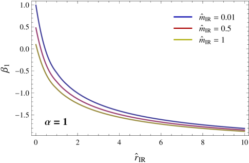
Figure 2: $\beta_{1}\equiv\int_{0}^{\infty}\!dt\,t^{3}\left[\tilde{K}^{IR}_{\alpha=1}(t)/\tilde{I}^{IR}_{\alpha=1}(t)\right]$ as a function of $\hat{r}_{IR}$ for three values of $\hat{m}_{IR}$.

$\bullet$ High-scale SUSY breaking on the UV brane: We consider a region where $L>L_{T}$, where $L_{T}$ is defined in Eq. (21), so that Eq. (22) applies for the superpartner with a non-vanishing UV mass term. Taking for concreteness the case $\alpha=1$, so that Eq. (24) applies to the superpartner with no mass terms (e.g. the gauge field), we see that

$$\Delta V_{\rm Casimir}(L) \approx \left.V_{\rm Casimir}(L)\right|_{\hat{r}_{i},\hat{m}_{i}=0}\leavevmode\nobreak\ \approx\leavevmode\nobreak\ -\frac{k^{4}e^{-4kL}}{16\pi^{2}}\,\frac{1}{kL+\hat{r}_{UV}}\int_{0}^{\infty}\!dt\,t^{3}\frac{\tilde{K}^{IR}_{\alpha=1}(t)}{\tilde{I}^{IR}_{\alpha=1}(t)}\leavevmode\nobreak\ ,$$ (38)

since the term $\left.-V_{\rm Casimir}(L)\right|_{\hat{r}_{i},\hat{m}_{i}}$ gives an exponentially small contribution (suppressed by $e^{-2kL}$, as remarked in the paragraph after Eq. (LABEL:VCasSmallmUV1alpha2) of Subsection 2.3). This is essentially the result derived in Ref. [14], although here we allow for a non-vanishing $\hat{r}_{UV}$. If SUSY is unbroken on the IR brane, the first term in Eq. (37) vanishes, and the radion is not stabilized. Depending on the size of the IR BKT, which can change the sign of the integral in Eq. (38), the branes can collapse towards each other or “run-away”.

However, if SUSY is also broken on the IR brane, one can realize the scenario envisioned in Ref. [14]. In this case, the radion potential, Eq. (12), has an extremum at $kL\approx\beta_{1}/\Delta-\hat{r}_{UV}$, provided $\beta_{1}/\Delta>0$, where $\Delta=(\Lambda/k)^{2}u\,\hat{m}_{IR}$, and $\beta_{1}\equiv\int_{0}^{\infty}\!dt\,t^{3}\left[\tilde{K}^{IR}_{\alpha=1}(t)/\tilde{I}^{IR}_{\alpha=1}(t)\right]$. This extremum is a minimum when both $\beta_{1}$ and $\Delta$ are negative. The calculable coefficient $\beta_{1}$ can indeed be negative if there is a non-negligible $\hat{r}_{IR}$ or a sizable $\hat{m}_{IR}$, as shown in Fig. 2. Obtaining a minimum with $kL\sim 30$ requires that $|\Delta|\sim 1/30$, which can arise from a suppression due to $\hat{m}_{IR}\ll 1$. Note that having $\hat{m}_{IR}\ll 1$ does not mean that the superpartner (e.g the gaugino) is light, since we are assuming that there is a “large” source of SUSY breaking on the UV brane (more precisely, $e^{2kL}\hat{m}_{UV}\gg 1$). In fact, Table. 1 of Appendix A indicates that the physical soft breaking mass is of order the KK scale, $M_{\rm KK}\sim 2\times k\,e^{-kL}$, although there is a region where the soft mass can be parametrically smaller, of order $k\,e^{-kL}/\sqrt{kL}$.

$\bullet$ Low-scale SUSY breaking from the UV brane: We now consider SUSY breaking on the UV brane only (i.e. $\hat{m}_{IR}=0$, so that the incalculable contribution to the radion potential vanishes), and focus on the case that $kL\gg 1$ with $L\ll L_{T}$, as defined in Eq. (21) ($\hat{m}_{UV}$ so small that there is a light state in the spectrum). As remarked in the discussion after Eq. (LABEL:VCasSmallmUV1alpha2), the leading order contributions cancel within a given supermultiplet. We can therefore immediately obtain the leading effect in $\hat{m}_{UV}$ from Eqs. (79) and (80) of Appendix B, for the various possible localizations of the would-be zero mode. For instance, for IR localization, $0<\alpha<1$:

$$\Delta V_{\rm eff}(L;\hat{r}_{i},\hat{m}_{UV},\hat{m}_{IR}=0) \approx -\frac{k^{4}e^{-2(2-\alpha)kL}}{16\pi^{2}}\,\frac{4^{\alpha}\hat{m}_{UV}\sin^{2}(\pi\alpha)\Gamma(\alpha)^{2}}{\pi^{2}}\int_{0}^{\infty}\!dt\,t^{3-2\alpha}\frac{\tilde{K}^{IR}_{\alpha}(t)}{\tilde{I}^{IR}_{\alpha}(t)}\leavevmode\nobreak\ ,$$ (39)

for the flat case, $\alpha=1$:

$$\Delta V_{\rm eff}(L;\hat{r}_{i},\hat{m}_{UV},\hat{m}_{IR}=0) \approx -\frac{k^{4}e^{-2kL}}{16\pi^{2}}\,\frac{\hat{m}_{UV}}{(kL+\hat{r}_{UV})^{2}}\int_{0}^{\infty}\!dt\,t\,\frac{\tilde{K}^{IR}_{\alpha=1}(t)}{\tilde{I}^{IR}_{\alpha=1}(t)}\leavevmode\nobreak\ ,$$ (40)

and for “moderate” UV localization, $1<\alpha<2$:

$$\Delta V_{\rm eff}(L;\hat{r}_{i},\hat{m}_{UV},\hat{m}_{IR}=0) \approx$$ (41)

$$-\frac{k^{4}e^{-2\alpha kL}}{16\pi^{2}}\,\frac{4^{2-\alpha}(\alpha-1)\hat{m}_{UV}}{\Gamma(\alpha)\left[\Gamma(\alpha-1)+2\hat{r}_{UV}\Gamma(\alpha)\right][1+2\hat{r}_{UV}(\alpha-1)]}\int_{0}^{\infty}\!dt\,t^{2\alpha-1}\frac{\tilde{K}^{IR}_{\alpha}(t)}{\tilde{I}^{IR}_{\alpha}(t)}\leavevmode\nobreak\ .$$

For $\alpha\geq 2$, one also obtains $\Delta V_{\rm eff}(L;\hat{r}_{i},\hat{m}_{UV},\hat{m}_{IR}=0)\sim e^{-2\alpha kL}$. Note that the warp factor dependence is the same for $\alpha=1+\delta\alpha$ and $\alpha=1-\delta\alpha$, for any $\delta\alpha$, although the coefficients do not exhibit this symmetry. In the above formulas it is understood that $\hat{m}_{IR}=0$ in $\tilde{K}^{IR}_{\alpha}$ and $\tilde{I}^{IR}_{\alpha}$. It is clear that these potentials do not have a minimum by themselves. Nevertheless, note that from the point of view of the warp factor dependence, the case $\alpha=1$ gives the largest contribution. Furthermore, notice the “double-volume” suppression in Eq. (40). These properties are important when there are other quantum mechanical sources of radion stabilization [11]. We also point out that the coefficient of Eq. (40) can have either sign, since for instance

$$\int_{0}^{\infty}\!dt\,t\,\frac{\tilde{K}^{IR}_{\alpha=1}(t)}{\tilde{I}^{IR}_{\alpha=1}(t)} \longrightarrow \left\{\begin{array}[]{lcl}+0.63&&\textrm{for }\hat{r}_{IR}=0\\[5.0pt] -0.10&&\textrm{for }\hat{r}_{IR}=1\end{array}\right.\leavevmode\nobreak\ .$$ (44)

We now turn to the last scenario we wish to consider:

$\bullet$ SUSY breaking from the IR brane only: When $\hat{m}_{UV}=0$, but $\hat{m}_{IR}\ll 1$, the effective potential is determined by the term linear in $\hat{m}_{IR}$ of Eqs. (23), (24) and (LABEL:VCasSmallmUV1alpha2). For instance, in the case of a vector multiplet with $\alpha=1$, and for $kL\gg 1$, we have

$$\Delta V_{\rm eff}(L;\hat{r}_{i},\hat{m}_{UV}=0,\hat{m}_{IR}) \approx \frac{k^{4}e^{-4kL}}{16\pi^{2}}\left[\frac{\Lambda^{2}}{k^{2}}u\,\hat{m}_{IR}-\frac{B_{IR}\,\hat{m}_{IR}}{kL+\hat{r}_{UV}}\right]\leavevmode\nobreak\ ,$$ (45)

where [we set $\hat{m}_{IR}=0$ in $\tilde{I}^{IR}_{1}(t)^{2}$]

$$B_{IR} = \int_{0}^{\infty}\!dt\,\frac{t^{3}}{\tilde{I}^{IR}_{1}(t)^{2}}\leavevmode\nobreak\ \longrightarrow\leavevmode\nobreak\ \left\{\begin{array}[]{ccc}1.26&\textrm{for }\hat{r}_{IR}=0\\[5.0pt] 0.48&\textrm{for }\hat{r}_{IR}=1\end{array}\right.$$ (48)

is manifestly positive. In fact, for arbitrary $\hat{m}_{IR}$ the Casimir energy part of the potential (i.e. the difference between Eq. (24) at $\hat{m}_{IR}=0$ and the same expression at arbitrary $\hat{m}_{IR}$) is always negative. Thus, if $u<0$ this potential does not have an extremum in the physical (positive) region for $L$. However, if $u>0$ the effective potential exhibits a maximum. It follows that the contribution due to matter hypermultiplets with $\alpha=1$ (which has an overall minus sign relative to the gauge case, see footnote 5) has a minimum. Hence, a model with more matter degrees of freedom (with $\alpha\approx 1$) than gauge degrees of freedom can stabilize the size of the extra dimension through these quantum effects. However, for this minimum to be at $kL\gg 1$ (for self-consistency with the above approximations), one must have $u\Lambda^{2}/k^{2}\ll 1$. For small $kL$, where fields with different localization parameters $\alpha$ can give comparable contributions to the radion potential, stabilization may be possible as in the flat $S^{1}/Z_{2}$ orbifold case [30].

5 Conclusions

In this work, we examined the use of supersymmetry to control vacuum energy contributions to the radion potential. Our analysis included UV- and IR-brane-localized mass terms, to implement soft supersymmetry breaking, as well as localized kinetic terms. We found that UV-brane breaking of supersymmetry leads to a diminished Casimir energy contribution to the radion potential, both through the size of the soft terms, as well as through an additional volume suppression. This finding may be useful in constructing models where dynamical EWSB induces a non-trivial radion potential that is protected from unwanted large corrections, thus tying the Planck-weak scale hierarchy to the dynamics of EWSB itself [11]. As another possibility, we studied the question of quantum radion stabilization by bulk fields (without VEV’s). Stabilizing the radion at $kL\gg 1$ through the quantum effects studied in this paper requires that SUSY be broken on the IR brane. If in addition SUSY is also broken on the UV brane, the radion stabilization mechanism by flat fields of Ref. [14] can be easily realized, provided the sign of an incalculable contribution is favorable. Our results are sufficiently general to be applicable to fields of arbitrary spin, and obeying arbitrary boundary conditions, and can be expected to be useful also outside the SUSY context.

Note added: After posting the initial version of this work, we found that some contributions were missing in our brane-tension renormalization. These contributions signal that, absent exact supersymmetry, quantum corrections to brane-tensions are not well-defined in our effective theory, as may also be inferred on general grounds. We have clarified this point in the new version and removed discussions dealing with brane-tension renormalization, since they do not affect our main conclusions outlined in the abstract.

Acknowledgements

We thank Markus Luty for useful discussions. The work of H.D. is supported by the United States Department of Energy under Grant Contract DE-AC02-98CH10886. E.P. is supported by DOE under contract DE-FG02-92ER-40699.

Appendix A Scalar Fields with Brane-Localized Terms

In this appendix we collect, for reference, various details of the KK decomposition of a scalar field with arbitrary localized terms. We also give approximate analytical expressions for the lightest KK mass and the corresponding KK eigenfunction.

A.1 KK Decomposition

The action of Eq (2) for the scalar field, $\Phi$, is supplemented by the boundary conditions

$$\left.(\partial_{y}\Phi-M_{0}\Phi-r_{UV}\Box\Phi)\right|_{y=0}=0\leavevmode\nobreak\ ,\hskip 28.45274pt\left.(\partial_{y}\Phi+M_{L}\Phi+e^{2kL}r_{IR}\Box\Phi)\right|_{y=L}=0\leavevmode\nobreak\ ,$$ (49)

where $\Box=\eta^{\mu\nu}\partial_{\mu}\partial_{\nu}$. We write the KK decomposition for $\Phi$ as

$$\Phi(x^{\mu},y)=\frac{e^{ky}}{\sqrt{L}}\sum^{\infty}_{n=0}\phi^{n}(x^{\mu})f_{n}(y)\leavevmode\nobreak\ ,$$ (50)

where we pulled out an explicit factor $e^{ky}$ for convenience. The $\phi^{n}$ obey the Klein-Gordon equation $(\Box+m^{2}_{n})\phi^{n}=0$, while the KK wavefunctions satisfy

$$f^{\prime\prime}_{n}-2kf^{\prime}_{n}-(3k^{2}+M^{2})f_{n}=-e^{2ky}m^{2}_{n}f_{n}\leavevmode\nobreak\ ,$$ (51)

and are explicitly given by

$$f_{n}(y)=A_{n}e^{ky}\left[J_{\alpha}\!\left(\frac{m_{n}}{k}e^{ky}\right)+B_{n}\,Y_{\alpha}\!\left(\frac{m_{n}}{k}e^{ky}\right)\right]\leavevmode\nobreak\ ,$$ (52)

where $\alpha$ was defined in Eqs. (5) and (6), and $A_{n}$ is a normalization constant, determined from

$$\frac{1}{L}\int^{L}_{0}\!dyf_{n}(y)f_{m}(y)=\delta_{nm}\leavevmode\nobreak\ .$$ (53)

In terms of the definitions (6) and (10), the boundary conditions of Eq. (49), become

$$\partial_{y}f_{n}|_{y=0} = -\left[\left(\alpha-1\right)+b_{UV}\left(\frac{m_{n}}{k}\right)\right]kf_{n}(0)\leavevmode\nobreak\ ,$$ (54)

$$\partial_{y}f_{n}|_{y=L} = -\left[\left(\alpha-1\right)-b_{IR}\left(\frac{m_{n}}{k}e^{kL}\right)\right]kf_{n}(L)\leavevmode\nobreak\ ,$$ (55)

which determine the constant $B_{n}$ in Eq. (52) and the spectrum $m_{n}$ according to

$$B_{n}=-\frac{\tilde{J}^{UV}_{\alpha}\!\left(\frac{m_{n}}{k}\right)}{\tilde{Y}^{UV}_{\alpha}\!\left(\frac{m_{n}}{k}\right)}=-\frac{\tilde{J}^{IR}_{\alpha}\!\left(\frac{m_{n}}{k}e^{kL}\right)}{\tilde{Y}^{IR}_{\alpha}\!\left(\frac{m_{n}}{k}e^{kL}\right)}\leavevmode\nobreak\ ,$$ (56)

where we used the definitions (8) and (9) for $\tilde{J}^{UV}_{\alpha}$, $\tilde{J}^{IR}_{\alpha}$, $\tilde{Y}^{UV}_{\alpha}$ and $\tilde{Y}^{IR}_{\alpha}$.

A.2 Lightest KK Modes

The second equation in (56) determines the mass eigenvalues $m_{n}$. In particular, when $m_{UV}=m_{IR}=0$, one finds that $m_{0}=0$ is a solution. For non-zero but small $m_{UV}$ or $m_{IR}$ there is an eigenstate with mass $m_{0}\ll k\,e^{-kL}$. In this limit we can also obtain the approximate profile for the light mode by setting $m_{n}\approx 0$ in Eq. (51), which is then solved by

$$f_{0}(y) \approx \sqrt{\frac{2kL(1-\alpha)}{e^{2(1-\alpha)kL}-1}}\,e^{(1-\alpha)ky}\leavevmode\nobreak\ ,$$ (57)

where we also imposed the boundary conditions (54) and (55) with $m_{UV}=m_{IR}=0$, and normalized according to Eq. (53). We see that this is the same profile as that for a zero-mode fermion with a bulk Dirac mass $M=ck$, where $c=\alpha-1/2$, and in particular that the state is localized near the UV (IR) brane for $c>1/2$ ($c<1/2$). The case $c=1/2$ corresponds to a flat profile, $f_{0}(y)=1$.

	$m_{UV}\neq 0$ and $m_{IR}=0$	$m_{UV}=0$ and $m_{IR}\neq 0$
$\alpha>1$ (i.e. $c>1/2$)	$\displaystyle\sqrt{\frac{4\alpha e^{2kL}\hat{m}_{UV}}{e^{2kL}\hat{m}_{UV}+2\alpha/(\alpha-1)}}$	$\displaystyle\sqrt{\frac{4\alpha(\alpha-1)\hat{m}_{IR}}{-\alpha(2+\hat{m}_{IR})+(2\alpha+\hat{m}_{IR})e^{2(\alpha-1)kL}}}$
$\alpha=1$ (i.e. $c=1/2)$	$\displaystyle\sqrt{\frac{4e^{2kL}\hat{m}_{UV}}{e^{2kL}\hat{m}_{UV}+4kL}}$	$\displaystyle\sqrt{\frac{4\hat{m}_{IR}}{2(2+\hat{m}_{IR})kL-\hat{m}_{IR}}}$
$\alpha<1$ (i.e. $c<1/2$)	$\displaystyle\sqrt{\frac{4\alpha e^{2\alpha kL}\hat{m}_{UV}}{e^{2\alpha kL}\hat{m}_{UV}-2\alpha/(\alpha-1)}}$	$\displaystyle\sqrt{\frac{4(1-\alpha)\hat{m}_{IR}}{2+\hat{m}_{IR}}}$

Table 1: Would-be zero mode mass, $m_{0}$, in units of $k\,e^{-kL}$.

We can obtain an analytical approximation to the mass $m_{0}$ when $m_{UV}$ or $m_{IR}$ are small, by using the small argument approximation for the Bessel functions. In Table 1, we summarize the results for $m_{0}/(k\,e^{-kL})$ for the cases $\alpha>1$ (i.e. $c>1/2$), $\alpha=1$ (i.e. $c=1/2$) and $\alpha<1$ (i.e. $c<1/2$) when one of the UV or IR brane-localized masses is non-vanishing, but the other one vanishes. For simplicity, we set the brane kinetic terms to zero. We see that for non-vanishing $m_{UV}$, the criterion for these solutions to be valid (that they be small compared to $k\,e^{-kL}$) requires that $e^{2kL}\hat{m}_{UV}$ be small when $\alpha\geq 1$, while for $\alpha<1$ one needs $e^{2\alpha kL}\hat{m}_{UV}\ll 1$. This is related to the transition length $L_{T}$ defined in Eq. (21). Note also that when $m_{IR}\neq 0$ and $\alpha>1$, $m_{0}$ is exponentially small compared to $k\,e^{-kL}$, as long as $kL\gg 1$, due to the UV-localization of the corresponding wavefunction.

Appendix B Simple Expressions for the Radion Potential

In this appendix, we derive an analytic approximation to the radion potential that is sufficiently accurate for most applications and exhibits the radion dependence explicitly. We focus on the Casimir energy piece, Eq. (13), that we reproduce here for easy reference:

$$V_{\rm Casimir}(L) = \frac{k^{4}e^{-4kL}}{16\pi^{2}}\int_{0}^{\infty}\!dt\,t^{3}\ln\left|1-\frac{\tilde{K}^{IR}_{\alpha}(t)}{\tilde{I}^{IR}_{\alpha}(t)}\frac{\tilde{I}^{UV}_{\alpha}(te^{-kL})}{\tilde{K}^{UV}_{\alpha}(te^{-kL})}\right|\leavevmode\nobreak\ .$$ (58)

Note that the integral receives the main contribution from the region $0<t<{\rm few}$ as a consequence of the asymptotic behavior of the “IR factor”

$$\frac{\tilde{K}^{IR}_{\alpha}(t)}{\tilde{I}^{IR}_{\alpha}(t)} \sim -\frac{\hat{m}_{IR}-t+\hat{r}_{IR}t^{2}}{\hat{m}_{IR}+t+\hat{r}_{IR}t^{2}}\,\pi\,e^{-2t}\leavevmode\nobreak\ ,\hskip 28.45274pt\textrm{as }t\to\infty\leavevmode\nobreak\ ,$$ (59)

which implies that the integrand in Eq. (58) tends to zero exponentially for $t>{\rm few}$. It follows that, for $e^{-kL}\ll 1$, we can approximate the “UV factor” in Eq. (58) –which contains the radion dependence– by 

$$\frac{\tilde{I}^{UV}_{\alpha}(te^{-kL})}{\tilde{K}^{UV}_{\alpha}(te^{-kL})} \approx 4\left[\Xi(\alpha)-\frac{\Gamma(\alpha+1)}{\left(\frac{t}{2}\,e^{-kL}\right)^{2\alpha}}\,\frac{\Theta(\alpha)\Gamma(\alpha-1)t^{2}+2\Gamma(\alpha)\left(\hat{r}_{UV}t^{2}+e^{2kL}\hat{m}_{UV}\right)}{\hat{r}_{UV}t^{2}+e^{2kL}(\hat{m}_{UV}-2\alpha)}\right]^{-1}\leavevmode\nobreak\ ,$$ (64)

where $\Theta(\alpha)$ is the Heaviside step function (unity for $\alpha>0$, vanishing for $\alpha<0$), and

$$\Xi(\alpha) \equiv \left\{\begin{array}[]{lcl}\displaystyle 2\pi\csc(\pi\alpha)&&\textrm{for }0<|\alpha|<1\\[5.0pt] \displaystyle-\frac{4\pi e^{2kL}\alpha\csc(\pi\alpha)}{\hat{r}_{UV}t^{2}+e^{2kL}\left(\hat{m}_{UV}-2\alpha\right)}&&\textrm{for }1<\alpha<2\\[11.00008pt] \displaystyle 0&&\textrm{for }\alpha\geq 2\end{array}\right.\leavevmode\nobreak\ .$$ (68)

The cases $\alpha=0$ and $\alpha=1$ (and their very close vicinity) require special treatment:

$$\frac{\tilde{I}^{UV}_{\alpha=0}(te^{-kL})}{\tilde{K}^{UV}_{\alpha=0}(te^{-kL})} \approx \frac{(1/2-\hat{r}_{UV})\left(t\,e^{-kL}\right)^{2}-\hat{m}_{UV}}{1+\hat{m}_{UV}[kL-\gamma_{E}-\ln(t/2)]}\leavevmode\nobreak\ ,$$ (69)

$$\frac{\tilde{I}^{UV}_{\alpha=1}(te^{-kL})}{\tilde{K}^{UV}_{\alpha=1}(te^{-kL})} \approx -\frac{1}{2}\left(t\,e^{-kL}\right)^{2}\frac{\hat{r}_{UV}t^{2}+e^{2kL}(\hat{m}_{UV}-2)}{[kL+\hat{r}_{UV}-\gamma_{E}-\ln(t/2)]\,t^{2}+e^{2kL}\hat{m}_{UV}}\leavevmode\nobreak\ ,$$ (70)

while for $\alpha\leq-1$, the “UV factor” is $\hat{r}_{UV}$ and $\hat{m}_{UV}$-independent, and simply equals $(2/\pi)\sin(\pi\alpha)$. The cases were $\alpha$ is a negative integer, $-n$, should be understood as the limit $\alpha\to-n$. Eqs. (64)–(70) can be used as a starting point for further approximations that hold in different regimes of $L$. In particular, taking into account that $t$ is always of order one in the relevant region of integration, these expressions indicate that there is a transition in the $L$ dependence of the potential according to whether $L\gg L_{\rm T}$ or $L\ll L_{\rm T}$, where $L_{\rm T}$ is determined by $\hat{m}_{UV}$ according to Eq. (21) of the main text.

For $L\gg L_{\rm T}$ (i.e. $e^{2kL}\hat{m}_{UV}\gg 1$), the second term in the denominator of Eq. (64) can be approximated by $\left(\frac{t}{2}\,e^{-kL}\right)^{-2\alpha}$ $\left[2\hat{m}_{UV}\Gamma(\alpha)\Gamma(\alpha+1)\right]/\left[\hat{m}_{UV}-2\alpha\right]$. It follows that for $\alpha>0$ this second term dominates over $\Xi(\alpha)$, while for $\alpha<0$ the $\Xi(\alpha)$ term dominates. We then see that, for $\alpha>0$, the argument of the logarithm in Eq. (58) differs from unity by order $e^{-2\alpha kL}/\hat{m}_{UV}\ll 1$, and we can also safely Taylor expand it. Therefore, we can write for $L\gg L_{\rm T}$:

$$V^{\alpha>0}_{\rm Casimir} \approx \frac{k^{4}e^{-2(2+\alpha)kL}}{16\pi^{2}}\frac{2(\hat{m}_{UV}-2\alpha)}{2^{2\alpha}\hat{m}_{UV}\Gamma(\alpha)\Gamma(\alpha+1)}\int_{0}^{\infty}\!dt\,t^{3+2\alpha}\frac{\tilde{K}^{IR}_{\alpha}(t)}{\tilde{I}^{IR}_{\alpha}(t)}\leavevmode\nobreak\ ,$$ (71)

which also holds for $\alpha=1$, while for $\alpha=0$ one can use

$$V^{\alpha=0}_{\rm Casimir} \approx \frac{k^{4}e^{-4kL}}{16\pi^{2}}\frac{\hat{m}_{UV}}{1+\hat{m}_{UV}(kL-\gamma_{E})}\int_{0}^{\infty}\!dt\,t^{3}\frac{\tilde{K}^{IR}_{\alpha=0}(t)}{\tilde{I}^{IR}_{\alpha=0}(t)}\leavevmode\nobreak\ .$$ (72)

Here, for simplicity, we neglected the $\ln(t/2)$ term in Eq. (69), which introduces a modest error (it is easy to keep it under the integral for numerical evaluation, if necessary). For negative index, when the $\Xi(\alpha)$ term in Eq. (64) dominates, we have instead

$$V^{\alpha<0}_{\rm Casimir} \approx \frac{k^{4}e^{-4kL}}{16\pi^{2}}\int_{0}^{\infty}\!dt\,t^{3}\ln\left|1-\frac{2\sin(\pi\alpha)}{\pi}\,\frac{\tilde{K}^{IR}_{\alpha}(t)}{\tilde{I}^{IR}_{\alpha}(t)}\right|\leavevmode\nobreak\ .$$ (73)

In the complementary regime, $L\ll L_{T}$, we need to distinguish several cases. Keeping up to linear order in $\hat{m}_{UV}$, we have that $\tilde{I}^{UV}_{\alpha}(te^{-kL})/\tilde{K}^{UV}_{\alpha}(te^{-kL})$ can be approximated by

$$\left\{\begin{array}[]{lcl}\displaystyle\frac{1}{2}e^{-2kL}(1-2\hat{r}_{UV})t^{2}-\hat{m}_{UV}\leavevmode\nobreak\ ,&&\textrm{for }\alpha=0\leavevmode\nobreak\ ,\\[15.00002pt] \displaystyle\frac{2\sin(\pi\alpha)}{\pi}\left[1-\frac{\sin(\pi\alpha)\Gamma(\alpha)^{2}}{2\pi}\left(\frac{t}{2}\right)^{-2\alpha}e^{2\alpha kL}\hat{m}_{UV}\right]\leavevmode\nobreak\ ,&&\textrm{for }0<|\alpha|<1\leavevmode\nobreak\ ,\\[15.00002pt] \displaystyle\frac{1}{kL+\hat{r}_{UV}-\gamma_{E}-\ln(t/2)}\left[1-\frac{e^{2kL}\hat{m}_{UV}}{t^{2}\left(kL+\hat{r}_{UV}-\gamma_{E}-\ln(t/2)\right)}\right]\leavevmode\nobreak\ ,&&\textrm{for }\alpha=1\leavevmode\nobreak\ ,\\[15.00002pt] \displaystyle\frac{2e^{-2(\alpha-1)kL}}{\Gamma(\alpha)\left[\Gamma(\alpha-1)+2\hat{r}_{UV}\Gamma(\alpha)\right]}\left(\frac{t}{2}\right)^{2(\alpha-1)}\left[1-\frac{2(\alpha-1)e^{2kL}\hat{m}_{UV}}{t^{2}[1+2\hat{r}_{UV}(\alpha-1)]}\right]\leavevmode\nobreak\ ,&&\textrm{for }1<\alpha<2\leavevmode\nobreak\ ,\\[15.00002pt] \displaystyle\frac{2e^{-2(\alpha-1)kL}}{\Gamma(\alpha)\Gamma(\alpha-1)\left[1+2\hat{r}_{UV}(\alpha-1)\right]}\left(\frac{t}{2}\right)^{2(\alpha-1)}\left[1-\frac{2(\alpha-1)e^{2kL}\hat{m}_{UV}}{t^{2}\left[1+2\hat{r}_{UV}(\alpha-1)\right]}\right]\leavevmode\nobreak\ ,&&\textrm{for }\alpha\geq 2\leavevmode\nobreak\ .\end{array}\right.$$ (79)

When $\alpha>0$, these approximations assume that $t^{2}\gg e^{2kL}\hat{m}_{UV}$ (for $\alpha\geq 1$) or $t^{2\alpha}\gg e^{2\alpha kL}\hat{m}_{UV}$ (for $0<\alpha<1$), and therefore they fail for very small $t$. However, due to the $t^{3}$ factor in Eq. (58) the contribution to the integral from the small $t$ region is negligible, and the above approximations can be used everywhere. One can see from the above expressions that the “UV factor” is very small compared to unity for $\alpha\geq 1$. Therefore, one can expand the logarithm in Eq. (58) as was done in the large $L$ region, so that for $L\ll L_{T}$ and $\alpha\geq 1$:

$$V_{\rm Casimir}(L) \approx -\frac{k^{4}e^{-4kL}}{16\pi^{2}}\int_{0}^{\infty}\!dt\,t^{3}\frac{\tilde{K}^{IR}_{\alpha}(t)}{\tilde{I}^{IR}_{\alpha}(t)}\frac{\tilde{I}^{UV}_{\alpha}(te^{-kL})}{\tilde{K}^{UV}_{\alpha}(te^{-kL})}\leavevmode\nobreak\ ,$$ (80)

where $\tilde{I}^{UV}_{\alpha}(te^{-kL})/\tilde{K}^{UV}_{\alpha}(te^{-kL})$ is replaced by the appropriate case in Eq. (79). In fact, this expression gives reasonably accurate results even for $0<\alpha<1$. For $\alpha<0$, one can use Eq. (73) since the term linear in $\hat{m}_{UV}$, which is non-vanishing only for $-1<\alpha<0$ [second line of Eq. (79)], gives an exponentially small correction. Specific applications that can be easily derived from the above expressions are further discussed in the main text.

References

• [1] L. Randall and R. Sundrum, Phys. Rev. Lett.  83, 3370 (1999) [arXiv:hep-ph/9905221].
• [2] H. Davoudiasl, J. L. Hewett and T. G. Rizzo, Phys. Lett.  B 473, 43 (2000) [arXiv:hep-ph/9911262];
• [3] A. Pomarol, Phys. Lett.  B 486, 153 (2000) [arXiv:hep-ph/9911294].
• [4] Y. Grossman and M. Neubert, Phys. Lett.  B 474, 361 (2000) [arXiv:hep-ph/9912408].
• [5] T. Gherghetta and A. Pomarol, Nucl. Phys.  B 586 (2000) 141 [arXiv:hep-ph/0003129].
• [6] Y. Bai, M. Carena and E. Pontón, Phys. Rev.  D 81, 065004 (2010) [arXiv:0809.1658 [hep-ph]].
• [7] H. Davoudiasl and E. Pontón, Phys. Lett.  B 680, 247 (2009) [arXiv:0903.3410 [hep-ph]].
• [8] H. Davoudiasl, J. L. Hewett and T. G. Rizzo, Phys. Rev.  D 68, 045002 (2003) [arXiv:hep-ph/0212279].
• [9] M. S. Carena, E. Pontón, T. M. P. Tait and C. E. M. Wagner, Phys. Rev.  D 67 (2003) 096006 [arXiv:hep-ph/0212307]; M. S. Carena, A. Delgado, E. Pontón, T. M. P. Tait and C. E. M. Wagner, Phys. Rev.  D 68, 035010 (2003) [arXiv:hep-ph/0305188].
• [10] M. S. Carena, A. Delgado, E. Pontón et al., Phys. Rev.  D71, 015010 (2005). [hep-ph/0410344].
• [11] H. Davoudiasl and E. Pontón, work in progress.
• [12] J. Garriga, O. Pujolas and T. Tanaka, Nucl. Phys.  B 605, 192 (2001) [arXiv:hep-th/0004109].
• [13] W. D. Goldberger and I. Z. Rothstein, Phys. Lett.  B 491, 339 (2000) [arXiv:hep-th/0007065].
• [14] J. Garriga and A. Pomarol, Phys. Lett.  B 560, 91 (2003) [arXiv:hep-th/0212227].
• [15] N. Maru and Y. Sakamura, JHEP 1004, 100 (2010) [arXiv:1002.4259 [hep-ph]].
• [16] W. D. Goldberger, M. B. Wise, Phys. Rev. Lett.  83, 4922-4925 (1999). [hep-ph/9907447].
• [17] A. Flachi, J. Garriga, O. Pujolas and T. Tanaka, JHEP 0308, 053 (2003) [arXiv:hep-th/0302017].
• [18] T. Gregoire, R. Rattazzi, C. A. Scrucca, A. Strumia and E. Trincherini, Nucl. Phys.  B 720, 3 (2005) [arXiv:hep-th/0411216].
• [19] A. Katz, Y. Shadmi and Y. Shirman, Phys. Rev.  D 75, 055008 (2007) [arXiv:hep-th/0601036].
• [20] F. del Aguila, M. Perez-Victoria and J. Santiago, JHEP 0302, 051 (2003) [arXiv:hep-th/0302023].
• [21] N. Arkani-Hamed, T. Gregoire and J. G. Wacker, JHEP 0203, 055 (2002) [arXiv:hep-th/0101233].
• [22] D. Marti and A. Pomarol, Phys. Rev.  D 64, 105025 (2001) [arXiv:hep-th/0106256].
• [23] E. A. Mirabelli, M. E. Peskin, Phys. Rev.  D58, 065002 (1998). [hep-th/9712214].
• [24] R. D’Auria, E. Maina, T. Regge et al., Annals Phys.  135, 237-269 (1981).
• [25] R. Altendorfer, J. Bagger and D. Nemeschansky, Phys. Rev.  D 63, 125025 (2001) [arXiv:hep-th/0003117].
• [26] J. Bagger, F. Feruglio and F. Zwirner, JHEP 0202, 010 (2002) [arXiv:hep-th/0108010].
• [27] S. De Curtis, D. Dominici, J. R. Pelaez, JHEP 0401, 052 (2004). [hep-th/0311226].
• [28] K. Choi, J. E. Kim and H. P. Nilles, Phys. Rev. Lett.  73, 1758 (1994) [arXiv:hep-ph/9404311].
• [29] K. A. Intriligator and N. Seiberg, Class. Quant. Grav.  24, S741 (2007) [arXiv:hep-ph/0702069].
• [30] E. Pontón, E. Poppitz, JHEP 0106, 019 (2001). [hep-ph/0105021].