Constrained-Pairing Mean-Field Theory. IV. Inclusion of corresponding pair constraints and connection to unrestricted Hartree-Fock theory

Abstract

Our previously developed Constrained-Pairing Mean-Field Theory (CPMFT) is shown to map onto an Unrestricted Hartree-Fock (UHF) type method if one imposes a corresponding pair constraint to the correlation problem that forces occupation numbers to occur in pairs adding to 1. In this new version, CPMFT has all the advantages of standard independent particle models (orbitals and orbital energies, to mention a few), yet unlike UHF, it can dissociate polyatomic molecules to the correct ground-state restricted open-shell Hartree-Fock atoms or fragments.

I Introduction

In a recent series of papers,CPMFT1 ; CPMFT2 ; CPMFT3 we have developed constrained-pairing mean-field theory (CPMFT), a method capable of describing static (strong) correlation in an accurate and efficient manner. The idea behind CPMFT is to make use of the pairing correlations (see below) that occur in a quasiparticle picture to describe static correlation in molecular systems. In CPMFT, we divide the natural orbitals into core, active, and virtual blocks; each core orbital has unit occupation, each virtual orbital has zero occupation, and the active natural orbitals have fractional occupations $n_{i}$, where $0<n_{i}<1$. Static correlation is introduced by allowing electron pairs to have fractional occupations within an active space.

The use of a pairing interaction has many advantages. Unlike unrestricted Hartree-Fock (UHF), CPMFT has zero spin density everywhere for closed-shell systems. In the absence of static correlation, CPMFT reduces to restricted Hartree-Fock (RHF), while it dissociates polyatomic molecules to restricted open shell Hartree-Fock (ROHF) atoms or fragments. Essentially, the dissociation limit of CPMFT can be thought of as an ensemble solution. By reducing to RHF in the absence of strong correlation and ROHF at dissociation, CPMFT cleanly separates static from dynamic correlation, as previously shown in Ref. CPMFT3, , where the CPMFT $\mathbf{P}$ and $\mathbf{K}$ density matrices were used to construct alternative densities to be used as inputs into traditional density functionals for the dynamical correlation energy. Remarkably, CPMFT accomplishes these feats at a mean field computational cost instead of the combinatorial blowup of complete active space (CASSCF) or full configuration interaction (FCI).

While CPMFT is clearly distinct from UHF, it shows some unexpected connections. We can take advantage of these connections to simplify the formalism, make it more efficient, and establish interesting similarities. The purpose of this paper is to demonstrate these relations and the accompanying reformulation of CPMFT. Accordingly, we discuss this connection in Sec. III at some length, and show how we can use it to simplify the solution of the CPMFT equations. Section IV shows some numerical examples, and we provide conclusions in Sec. V. We include an Appendix that discusses some other formal properties of CPMFT. First, however, we provide a brief introduction to pairing correlations in Sec. II.

II Pairing Correlations and the Quasiparticle Picture

Strong correlations in nuclear physics or superconductivity are often described as the formation of Cooper pairs. The theoretical machinery which does this is the Hartree-Fock-Bogoliubov (HFB) method.Blaizot In HFB, we write the wave function $|\Phi_{\mathrm{HFB}}\rangle$ as a single determinant of quasiparticles created by quasiparticle creation operators which are linear combinations of electron creation and annihilation operators. The quasiparticle wave function thus violates electron number conservation. Because the quasiparticle wave function is a single determinant, its associated density matrix $\mathbf{R}$ is idempotent ($\mathbf{R}^{2}=\mathbf{R}$) and Hermitian ($\mathbf{R}=\mathbf{R}^{\dagger}$). We have

$$\mathbf{R}=\begin{pmatrix}\bm{\gamma}&\bm{\kappa}\\ -\bm{\kappa}^{\star}&\bm{1}-\bm{\gamma}^{\star}\end{pmatrix}.$$ (1)

Here, $\bm{\gamma}$ is the physical density matrix in the spinorbital basis; it is Hermitian but not idempotent. Information about pairing correlations is carried by the anomalous density matrix $\bm{\kappa}$, which is antisymmetric by definition because $\kappa_{ij}=\langle a_{i}^{\dagger}a_{j}^{\dagger}\rangle$. We limit our discussion to the closed shell case, in which case we have, for $\alpha\alpha$, $\alpha\beta$, $\beta\alpha$, and $\beta\beta$ blocks

$$\bm{\gamma} =\begin{pmatrix}\mathbf{P}&\bm{0}\\ \bm{0}&\mathbf{P}\end{pmatrix},$$ (2a)

$$\bm{\kappa} =\begin{pmatrix}\bm{0}&\mathbf{K}\\ -\mathbf{K}&\bm{0}\end{pmatrix},$$ (2b)

where $\mathbf{P}$ is the closed-shell (spatial orbital) density matrix and $\mathbf{K}$ is the (symmetric, positive semi-definite) closed-shell anomalous density matrix. We emphasize here that only the $\alpha\beta$ and $\beta\alpha$ blocks of $\bm{\kappa}$ are non-zero, so that we consider only singlet pairing.SS2002 We should also mention that the notation here differs slightly from that used in Refs. CPMFT1, ; CPMFT2, ; CPMFT3, , but does so in an attempt to make this manuscript self-contained and as clear as possible.

Idempotence of the quasiparticle density matrix $\mathbf{R}$ yields two conditions on the electronic density matrix $\mathbf{P}$ and the anomalous density matrix $\mathbf{K}$:

$$\mathbf{P}\,\mathbf{K}-\mathbf{K}\,\mathbf{P} =\bm{0}$$ (3a)

$$\mathbf{P}-\mathbf{P}^{2} =\mathbf{K}^{2}.$$ (3b)

Physically, $\mathbf{K}^{2}$ is the “odd-electron distribution” of Yamaguchi,Yamaguchi the “density of effectively unpaired electrons” of Staroverov and Davidson,Star-David and is related to Mayer’s “free valence index”Mayer once it is written in terms of the total density matrix $\bm{\gamma}^{\alpha\alpha}+\bm{\gamma}^{\beta\beta}=2\mathbf{P}$. Essentially, $\mathbf{K}^{2}$ gauges the singlet diradical character of the system (or, for larger active spaces, the polyradical character) and is a local measure of electron entanglement.

The HFB energy is given as the expectation value of the Hamiltonian with respect to the HFB wave function

$$E_{\mathrm{HFB}} =\langle\Phi_{\mathrm{HFB}}|H|\Phi_{\mathrm{HFB}}\rangle$$ (4a)

$$=2h_{ij}P_{ij}+(2\langle ij|kl\rangle-\langle ij|lk\rangle)P_{ik}P_{jl}$$ (4b)

$$\qquad+\langle ij|kl\rangle K_{ij}K_{kl}$$

where summation over repeated indices here and throughout the manuscript is implied; $h_{ij}$ are matrix elements of the one-electron part of the Hamiltonian and $\langle ij|kl\rangle$ are two-electron integrals in Dirac notation.

In order to determine the occupation numbers and natural orbitals, HFB variationally minimizes $E_{\mathrm{HFB}}$ subject to the constraint that the density matrix $\mathbf{P}$ contains the correct number of particles:

$$\mathrm{Tr}(\mathbf{P})=N.$$ (5)

This condition is enforced by a chemical potential $\mu$ introduced as a Lagrange multiplier. The HFB formulation leads to equations similar to Hartree-Fock, which in the particular case of closed-shell systems are

$$\mathbf{R}_{\mathrm{cs}}\,\bm{\mathcal{H}}_{\mathrm{HFB}}-\bm{\mathcal{H}}_{\mathrm{HFB}}\,\mathbf{R}_{\mathrm{cs}}=\bm{0},$$ (6)

where $\mathbf{R}_{\mathrm{cs}}$ is the closed shell quasiparticle density matrix

$$\mathbf{R}_{\mathrm{cs}}=\begin{pmatrix}\mathbf{P}&\mathbf{K}\\ \mathbf{K}&\bm{1}-\mathbf{P}\end{pmatrix}$$ (7)

and $\bm{\mathcal{H}}_{\mathrm{HFB}}$ is the double-Hamiltonian (DH) given by

$$\bm{\mathcal{H}}_{\mathrm{HFB}}=\begin{pmatrix}\mathbf{F}^{\mathrm{cs}}+\mu N&\bm{\Delta}\\ \bm{\Delta}&-\mathbf{F}^{\mathrm{cs}}-\mu N\end{pmatrix}.$$ (8)

Here $\mathbf{F}^{\mathrm{cs}}$ is the standard closed-shell Fock matrix and $\bm{\Delta}$ is known as the pairing Hamiltonian. These are given by

$$F^{\mathrm{cs}}_{ij} =h_{ij}+(2\langle ik|jl\rangle-\langle ik|lj\rangle)P_{kl},$$ (9a)

$$\Delta_{ij} =\langle ij|kl\rangle K_{kl}.$$ (9b)

The double-Hamiltonian $\bm{\mathcal{H}}_{\mathrm{HFB}}$ is just the mean-field of the physical Hamiltonian with respect to the quasiparticle determinant.

Because the pairing energy of HFB (the term proportional to $\mathbf{K}^{2}$ in Eqn. (4b)) is positive when the electron-electron interaction is repulsive, the variationally optimal solution is always $\mathbf{K}=\bm{0}$ and therefore $\bm{\Delta}=\bm{0}$. In other words, HFB just returns the regular Hartree-Fock solution for Coulombic repulsive systems. In order to have HFB solutions with energies lower than Hartree-Fock, one needs a net attractive two-body interaction, as in the Bardeen-Cooper-Schriefer picture of superconductivity (where it is provided by electron-phonon coupling) or in nuclear forces. In order to take advantage of the pairing picture for the conventional repulsive electron-electron interaction, and with the aim of describing strong correlations, CPMFT simply reverses the sign of the pairing energy. We thus have

$$\begin{split}E_{\mathrm{CPMFT}}&=2h_{ij}P_{ij}+(2\langle ij|kl\rangle-\langle ij|lk\rangle)P_{ik}P_{jl}\\ &\qquad-\langle ij|kl\rangle K_{ij}K_{kl}\end{split}$$ (10)

The last term plays the role of a correlation energy – a correction to the closed shell RHF-like energy expression – and will be referred to as such throughout this manuscript, but it is certainly not our previous definition of static correlation,CPMFT2 $E_{\mathrm{CPMFT}}-E_{\mathrm{RHF}}$, since $\mathbf{P}$ is not $\mathbf{P}_{\mathrm{RHF}}$.

In addition to changing the sign of the pairing energy, in CPMFT we also restrict non-integer occupations to an active space, so that pairing only occurs between quasidegenerate orbitals. Changing the sign of the pairing term changes the sign of $\bm{\Delta}$ so that the double-Hamiltonian is

$$\bm{\mathcal{H}}_{\mathrm{CPMFT}}=\begin{pmatrix}\mathbf{F}^{\mathrm{cs}}+\mu N&-\bm{\Delta}\\ -\bm{\Delta}&-\mathbf{F}^{\mathrm{cs}}-\mu N\end{pmatrix}.$$ (11)

Otherwise, DH-CPMFT follows the same procedure as in HFB. However, changing the sign of the pairing energy and the pairing matrix severs the connection between the HFB wave function $|\Phi_{\mathrm{HFB}}\rangle$ and the CPMFT energy. Note that what we have called simply CPMFT in Refs. CPMFT1, ; CPMFT2, ; CPMFT3, is here referred to as DH-CPMFT, whereas “CPMFT” here refers to the new formulation to be introduced below.

We can, indeed, view the CPMFT energy as the expectation value of a model Hamiltonian with respect to a particle-number violating determinant:

$$H_{0}|\Phi\rangle =E_{\mathrm{CPMFT}}|\Phi\rangle,$$ (12a)

$$H_{0} =(F^{\mathrm{cs}}_{ij}+h_{ij})a_{i}^{\dagger}a_{j}$$ (12b)

$$-\frac{1}{2}\Delta_{ij}a_{i}^{\dagger}a_{j}^{\dagger}-\frac{1}{2}\Delta^{\star}_{ij}a_{i}a_{j}.$$

This quadratic model Hamiltonian, however, is not the mean-field of the physical Hamiltonian with respect to a quasiparticle determinant. As previously noted,CPMFT2 we can interpret the CPMFT energy as a hybrid of Hartree-Fock and HFB where Hartree-Fock uses $2/r_{12}$ as the electron-electron repulsion operator and HFB uses $-1/r_{12}$.

Nevertheless, we have a fruitful alternative viewpoint, which is to envision the CPMFT energy expression of Eqn. (10) as defining a model two-particle density matrix $\bm{\Gamma}$ such that the energy in the spin-orbital basis is

$$E_{\mathrm{CPMFT}}=\mathrm{Tr}(\mathbf{h}\,\bm{\gamma})+\mathrm{Tr}(\mathbf{v}\,\bm{\Gamma}_{\mathrm{CPMFT}})$$ (13)

where $\mathbf{v}$ is the two-particle part of the Hamiltonian, and $\mathbf{h}$ is the one-particle part. In terms of spin-orbitals, we have

$$(\bm{\Gamma}_{\mathrm{CPMFT}})_{ij}^{kl}=\frac{1}{2}\gamma_{i}^{k}\gamma_{j}^{l}-\frac{1}{2}\gamma_{i}^{l}\gamma_{j}^{k}-\frac{1}{2}\kappa_{ij}\kappa^{kl}$$ (14)

with lower (upper) indices corresponding to bra (ket) indices. The first two terms in this model two-particle density matrix correspond to Hartree-Fock whereas the last term introduces static correlation via $\mathbf{K}$, which is a measure of non-idempotency for $\mathbf{P}$. This last term is an important quantity in the cumulant decomposition of density matrices,Kutzelnigg but in our work appears naturally from the idempotency of the quasiparticle density matrix. If we use this model two-particle density matrix to define expectation values of two-particle operators, then as shown in the Appendix, we find the important result that CPMFT has no particle number fluctuations. In making this choice, we are inevitably working with a density matrix functional and are effectively doing some form of a statistical ensemble theory. Table 1 collects results about the UHF two-particle density matrix, the CPMFT model two-particle density matrix, and the analogously defined HFB model two-particle density matrix. We derive these results in the Appendix.

Table 1: Summary of properties in UHF, HFB, and CPMFT for closed-shell systems. We show the correlation energy (i.e the difference between the energy from the method and the closed-shell piece), the effective polarization, and the particle number fluctuations.

Method	$E_{c}$	Polarization	$\sigma_{N}^{2}$
UHF	$-v_{ij}^{kl}\,M^{i}_{l}\,M^{j}_{k}$	$\mathbf{M}=(\mathbf{A}-\mathbf{B})/2$	0
HFB	$v_{ij}^{kl}\,K^{ij}\,K_{kl}$	$\mathbf{K}=|\mathbf{A}-\mathbf{B}|/2$	$4\,\mathrm{Tr}(\mathbf{K}^{2})$
CPMFT	$-v_{ij}^{kl}\,K^{ij}\,K_{kl}$	$\mathbf{K}=|\mathbf{A}-\mathbf{B}|/2$	0

Note that our model two-particle density matrix has appeared before in the literature as the corrected Hartree-Fock (CHF) functional.CHF Our model is, however, solved by diagonalization.SS2002 More importantly, CPMFT restricts the non-integer occupation numbers to an active space only, and in the present work further enforces the corresponding pairs constraint, which we will now introduce.

III CPMFT and UHF

Consider the UHF treatment of a system where the number of spin-up and spin-down electrons is the same. The spin-up and spin-down density matrices $\bm{\gamma}^{\alpha\alpha}$ and $\bm{\gamma}^{\beta\beta}$ are both idempotent:

$$(\bm{\gamma}^{\alpha\alpha})^{2}-\bm{\gamma}^{\alpha\alpha}=(\bm{\gamma}^{\beta\beta})^{2}-\bm{\gamma}^{\beta\beta}=\bm{0}.$$ (15)

The charge density and spin magnetization (or polarization) density matrices are

$$\mathbf{P} =\frac{1}{2}\big{(}\bm{\gamma}^{\alpha\alpha}+\bm{\gamma}^{\beta\beta}\big{)}$$ (16a)

$$\mathbf{M} =\frac{1}{2}\big{(}\bm{\gamma}^{\alpha\alpha}-\bm{\gamma}^{\beta\beta}\big{)}.$$ (16b)

Traditionally, the UHF energyPople is expressed in terms of the $\bm{\gamma}^{\alpha\alpha}$ and $\bm{\gamma}^{\beta\beta}$ density matrices:

$$E_{\mathrm{UHF}} =h_{ij}(\gamma^{\alpha\alpha}_{ij}+\gamma^{\beta\beta}_{ij})$$ (17)

$$+\frac{1}{2}\langle ij|kl\rangle(\gamma^{\alpha\alpha}_{ik}+\gamma^{\beta\beta}_{ik})(\gamma^{\alpha\alpha}_{jl}+\gamma^{\beta\beta}_{jl})$$

$$-\frac{1}{2}\langle ij|kl\rangle(\gamma^{\alpha\alpha}_{il}\gamma^{\alpha\alpha}_{jk}+\gamma^{\beta\beta}_{il}\gamma^{\beta\beta}_{jk})$$

where we have put $\bm{\gamma}^{\alpha\alpha}$ and $\bm{\gamma}^{\beta\beta}$ in the same basis (say, the atomic orbital basis). Although it is almost never presented in this way, we can also write the UHF energy as a functional of $\mathbf{P}$ and $\mathbf{M}$, which yields

$$E_{\mathrm{UHF}}[\mathbf{P},\mathbf{M}] =E_{\mathrm{cs}}[\mathbf{P}]+E_{c}[\mathbf{M}],$$ (18a)

$$E_{\mathrm{cs}}[\mathbf{P}] =2h_{ij}P_{ij}$$ (18b)

$$+(2\langle ij|kl\rangle-\langle ij|lk\rangle)P_{ik}P_{jl}$$

$$E_{c}[\mathbf{M}] =-\langle ij|kl\rangle M_{il}M_{jk}.$$ (18c)

Here, $E_{\mathrm{cs}}$ indicates the usual RHF energy expression given in terms of the charge density matrix $\mathbf{P}$, while $E_{c}$ carries the correlation energy in terms of the spin magnetization density matrix $\mathbf{M}$. An utterly unexpected result is that the closed-shell CPMFT energy expression of Eqn. (10) is identical to the UHF energy expression of Eqn. (18), except that the spin density matrix $\mathbf{M}$ is replaced by the anomalous density matrix $\mathbf{K}$.FOOTNOTE In cases in which UHF predicts static correlation by breaking symmetry (i.e non-zero spin density),Fukutome $\mathbf{P}$ is not idempotent. Instead, it satisfies

$$\mathbf{P}-\mathbf{P}^{2} =\frac{1}{2}(\bm{\gamma}^{\alpha\alpha}+\bm{\gamma}^{\beta\beta})-\frac{1}{4}(\bm{\gamma}^{\alpha\alpha}+\bm{\gamma}^{\beta\beta})^{2}$$ (19a)

$$=\frac{1}{4}(\bm{\gamma}^{\alpha\alpha}-\bm{\gamma}^{\beta\beta})^{2}$$ (19b)

$$=\mathbf{M}^{2}.$$ (19c)

This is one consequence of the idempotence of $\bm{\gamma}^{\alpha\alpha}$ and $\bm{\gamma}^{\beta\beta}$. The second is

$$\mathbf{P}\,\mathbf{M}+\mathbf{M}\,\mathbf{P}=\mathbf{M}.$$ (20)

Note that the condition of Eqn. (19) is the same as the CPMFT condition of Eqn. (3b), again with $\mathbf{M}$ taking the role of $\mathbf{K}$. Both the magnetization density matrix $\mathbf{M}$ and the anomalous density matrix $\mathbf{K}$ are Hermitian.

While CPMFT and UHF thus use the same energy expression (one with $\mathbf{K}$ and the other with $\mathbf{M}$), $\mathbf{K}$ and $\mathbf{M}$ are not the same even though with the same density matrix $\mathbf{P}$, we have $\mathbf{K}^{2}=\mathbf{M}^{2}$. There are also some other important differences. Both UHF and CPMFT impose an additional condition on these two matrices, which in UHF is given in Eqn. (20) while in CPMFT is instead given in Eqn. (3a). Additionally, $\mathbf{K}$ is positive semi-definite while $\mathbf{M}$ is traceless (and thus has both positive and negative eigenvalues). Finally, because in UHF we write $\mathbf{P}$ as the half-sum of two idempotent matrices, its eigenvalues occur in what is known as “corresponding pairs” $n_{i}$ and $1-n_{i}$,Amos ; Harriman a terminology that we here adopt.

That UHF has the corresponding pairs property has little to do with UHF per se. It originates simply from the observationmath that the eigenvalues of a matrix that is the half-sum of two idempotent matrices are 0, 1, $\tfrac{1}{2}$, or a corresponding pair ($n,1-n$). Similarly, the eigenvalues of a matrix written as the half-difference of two idempotent matrices are 0, $\pm\tfrac{1}{2}$, or a corresponding pair ($-n,n$).FOOTNOTE2 Thus, for example, $\mathbf{M}$ has eigenvalues adding to 0 in pairs while $\mathbf{P}$ has eigenvalues adding to 1 in pairs. Quite generally, any non-integer eigenvalues of the charge density matrix from a single determinant method will be either $\tfrac{1}{2}$ or occur in a corresponding pair. Eigenvalues of $\tfrac{1}{2}$ could be part of a corresponding pair (for entangled electrons) or may occur singly for open shells. We should be clear that while matrices written as the sum of two idempotent matrices exhibit the corresponding pairs property, the converse is not necessarily true; a matrix whose eigenvalues come in corresponding pairs may or may not be the sum of two idempotents.

Unlike UHF, the eigenvalues of $\mathbf{P}$ in DH-CPMFT do not occur in corresponding pairs (except when the active space consists of two spatial orbitals). That said, the corresponding pairs property has some attractive features for CPMFT. Most important is that it eliminates overcorrelation between orbital pairs in different symmetries. This is ubiquitous for example in N₂ where the variational principle drives occupancy into orbitals at low energies and one must introduce multiple chemical potentials to retain the correct total number of $\sigma$ and $\pi$ electrons. A corresponding pair constraint controls this unphysical “spilling” and has the inherent attractive feature of limiting strong correlations to be an affair between orbital pairs.

Previously, we had introduced the corresponding pairs feature within the DH-CPMFT framework using different chemical potentials (Lagrange multipliers) for different irreducible representations of the system. However, in the general case where no spatial symmetry is present, imposition of this constraint leads to one Lagrange multiplier per orbital pair and a rather complicated nonlinear optimization problem. A more satisfactory and much simpler approach, however, is to write the CPMFT density matrix as

$$\mathbf{P}=\frac{1}{2}\left(\mathbf{A}+\mathbf{B}\right)$$ (21)

where $\mathbf{A}$ and $\mathbf{B}$ are auxiliary density matrices, individually idempotent and Hermitian ($\mathbf{A}^{2}=\mathbf{A}=\mathbf{A}^{\dagger}$ and similarly for $\mathbf{B}$). As with UHF, the decomposition above enforces the corresponding pairs condition automatically, and there is no need to enforce this condition via Lagrange multipliers. Eigenvalues of 0 or 1 in $\mathbf{P}$ correspond to virtual or core orbitals, respectively, while paired eigenvalues correspond to active orbitals. Further, by choosing $\mathbf{A}$ and $\mathbf{B}$ to trace to half the number of electrons, we guarantee that $\mathbf{P}$ does likewise, and we thus have no need of any chemical potential. By making this decomposition, in other words, we can avoid the Lagrange multipliers of the double-Hamiltonian approach entirely, and thus simplify the computation. Note that once we have converged solutions for $\mathbf{A}$ and $\mathbf{B}$ (and thus $\mathbf{P}$ and $\mathbf{K}$), we could, if desired, extract the Lagrange multipliers of the DH-CPMFT approach.

The critical mathematical difference between CPMFT as formulated in this manner and UHF is that in UHF, we get $\mathbf{M}$ from the spin-up and spin-down density matrices, while in CPMFT, we get $\mathbf{K}$ from the total density matrix alone (since $\mathbf{K}$ satisfies the condition of Eqn. (3b), commutes with $\mathbf{P}$, and is positive semi-definite). In other words, CPMFT with corresponding pairs defines $\mathbf{P}$ from $\mathbf{A}$ and $\mathbf{B}$ as in Eqn. (21), but differs from UHF in constructing

$$\mathbf{K}=\sqrt{\mathbf{P}-\mathbf{P}^{2}}=\frac{1}{2}\sqrt{(\mathbf{A}-\mathbf{B})^{2}}=\frac{1}{2}|\mathbf{A}-\mathbf{B}|.$$ (22)

from auxiliary density matrices $\mathbf{A}$ and $\mathbf{B}$ while UHF builds $\mathbf{P}$ and $\mathbf{M}$ from $\bm{\gamma}^{\alpha\alpha}$ and $\bm{\gamma}^{\beta\beta}$, as shown in Eqn. (16). Note in the last equation our definition of the absolute value of a matrix from the square root of the square. In practice, to calculate the absolute value of a matrix one needs to diagonalize it, flip the sign of the negative eigenvalues and transform back to the original basis. Both the square root and absolute value of a matrix are positive definite matrices and both have a convergent polynomial series expansion if the matrix is positive definite with eigenvalues between 0 and 1, as is the case here.

To make the comparison between CPMFT and UHF more concrete, consider the case where $\mathbf{A}$ and $\mathbf{B}$ are 2$\times$2 matrices and let $\mathbf{M}=\frac{1}{2}(\mathbf{A}-\mathbf{B})$. Idempotency of $\mathbf{A}$ and $\mathbf{B}$ requires that in the natural orbital basis we have

$$\mathbf{A} =\begin{pmatrix}n&k\\ k&1-n\end{pmatrix}$$ (23a)

$$\mathbf{B} =\begin{pmatrix}n&-k\\ -k&1-n\end{pmatrix}$$ (23b)

$$\mathbf{P} =\begin{pmatrix}n&0\\ 0&1-n\end{pmatrix}$$ (23c)

$$\mathbf{M} =\begin{pmatrix}0&k\\ k&0\end{pmatrix}$$ (23d)

$$\mathbf{K} =\begin{pmatrix}k&0\\ 0&k\end{pmatrix}$$ (23e)

$$k =\sqrt{n(1-n)}.$$ (23f)

When $\mathbf{A}$ and $\mathbf{B}$ are of larger dimension, then in the natural orbital basis they are block diagonal with 2$\times$2 blocks of the form given above. This is essentially a consequence of Eqn. (20), which in the natural basis becomes

$$(n_{i}+n_{j})M_{ij}=M_{ij}=\frac{1}{2}(A_{ij}-B_{ij}),$$ (24)

the solutions to which are $M_{ij}=0$ and $n_{i}+n_{j}=1$. Because we also have $A_{ij}+B_{ij}=2\,n_{i}\,\delta_{ij}$, we conclude that for $i\neq j$, we must either have $A_{ij}=B_{ij}=0$ or $n_{i}+n_{j}=1$ (in other words, the two eigenvalues form a corresponding pair). When the occupation numbers are degenerate, the natural orbitals are not uniquely defined and we can thus choose them such that $\mathbf{A}$ and $\mathbf{B}$ still have this structure. In the core (virtual) space, $\mathbf{A}=\mathbf{B}=\bm{1}$ ($\mathbf{A}=\mathbf{B}=\bm{0}$).

Before we continue to the working equations for CPMFT in this UHF-like framework, let us pause to make it explicit that CPMFT and UHF are different methods. While we have expressed the UHF energy as a density matrix functional, we could also write it as an expectation value

$$E_{\mathrm{UHF}}=\langle\Phi_{\mathrm{UHF}}|H|\Phi_{\mathrm{UHF}}\rangle$$ (25)

with $|\Phi_{\mathrm{UHF}}\rangle$ constrained to be a single determinant. This is not true of the CPMFT energy expression, and in fact there seems to be no wave function associated with CPMFT. This may seem somewhat surprising, in light of the intimate connection between CPMFT and HFB theory, in which there certainly is a wave function, albeit one which violates particle number conservation. As we have said, we lose the HFB wave function because we have by fiat changed the sign of the pairing energy. Additionally, unlike UHF, the spin density is zero everywhere for closed shells, even in the presence of static correlation.

One might wonder whether CPMFT is equivalent to projected UHF (PUHF). It is not. If one projects the UHF determinant onto a spin eigenfunction, one finds that the charge density matrix of the UHF determinant and the spin-projected state have the same eigenfunctions.Harriman Spin projection, in other words, changes only the occupation numbers of the charge density matrix, but not the natural orbitals. The fact that the UHF and CPMFT natural orbitals are different should lay to rest any concerns that CPMFT is just a projected UHF.

Another fundamental difference between CPMFT and UHF is the onset of the appearance of the solution with energy lower than RHF. As shown in our previous paper,CPMFT2 the CPMFT solution for a two-level model system appears when the RHF orbital energy gap reduces to

$$\varepsilon_{2}-\varepsilon_{1}<\frac{1}{2}\langle 11|11\rangle+\frac{1}{2}\langle 22|22\rangle+\langle 11|22\rangle,$$ (26)

whereas the UHF Coulson-Fischer instability point is determined by

$$\varepsilon_{2}-\varepsilon_{1}<\langle 12|12\rangle+\langle 11|22\rangle.$$ (27)

Because all two-electron integrals in the equations above are positive, the CPMFT solution appears inevitably when the orbital gap closes and strong correlation is manifest, such as along a dissociation curve.

III.1 Working Equations

Let us now return to the solution of the CPMFT equations in this UHF-like framework. For convenience, we repeat the energy expression here:

$$E_{\mathrm{CPMFT}}=E_{\mathrm{cs}}-\langle ij|kl\rangle K_{ij}K_{kl}.$$ (28)

We simply minimize the energy with respect to (idempotent) $\mathbf{A}$ and $\mathbf{B}$ matrices. The derivatives of $E_{\mathrm{cs}}$ in Eqn. (28) with respect to $\mathbf{A}$ and $\mathbf{B}$ give the usual closed-shell Fock matrix obtained from $\mathbf{P}$. That is

$$\frac{\partial E_{\mathrm{cs}}}{\partial A_{ij}\hfill}=\frac{\partial E_{\mathrm{cs}}}{\partial B_{ij}\hfill}=\frac{1}{2}\frac{\partial E_{\mathrm{cs}}}{\partial P_{ij}\hfill}=F_{ij}^{\mathrm{cs}}.$$ (29)

The differences with UHF arise from differentiating the last term of the CPMFT energy, which we shall call $E_{c}^{\mathrm{CPMFT}}$. Taking derivatives with respect to $\mathbf{A}$ leads to an effective potential $\tilde{\bm{\Delta}}$, given by

$$\tilde{\Delta}_{ij}=\frac{\partial E_{c}^{\mathrm{CPMFT}}}{\partial A_{ij}\hfill}=\frac{\partial E_{c}^{\mathrm{CPMFT}}}{\partial K_{kl}\hfill}\frac{\partial K_{kl}}{\partial A_{ij}}=-2\Delta_{kl}\frac{\partial K_{kl}}{\partial A_{ij}}.$$ (30)

This is essentially the same result that we get from differentiating $E_{c}^{\mathrm{UHF}}$ of Eqn. (18):

$$\frac{\partial E_{c}^{\mathrm{UHF}}}{\partial\gamma^{\alpha\alpha}_{ij}}=\frac{\partial E_{c}^{\mathrm{UHF}}}{\partial M_{kl}}\frac{\partial M_{kl}}{\partial\gamma^{\alpha\alpha}_{ij}}=-2\Delta_{kl}^{\mathrm{UHF}}\frac{\partial M_{kl}}{\partial\gamma^{\alpha\alpha}_{ij}}$$ (31)

where

$$\Delta_{kl}^{\mathrm{UHF}}=\langle km|nl\rangle M_{mn}=\langle kl|mn\rangle M_{mn}$$ (32)

looks just like $\bm{\Delta}$ except we replace $\mathbf{K}$ with $\mathbf{M}$. In UHF, however, we simply have

$$\frac{\partial M_{kl}}{\partial\gamma^{\alpha\alpha}_{ij}}=\frac{1}{2}\delta_{ik}\delta_{jl}$$ (33)

while in CPMFT the derivative of $\mathbf{K}$ with respect to $\mathbf{A}$ is obtained by differentiating both sides of $\mathbf{K}^{2}=\tfrac{1}{4}(\mathbf{A}-\mathbf{B})^{2}$. This gives

$$\frac{\partial K_{km}}{\partial A_{ij}}K_{ml}+K_{km}\frac{\partial K_{ml}}{\partial A_{ij}}=\frac{1}{2}\left(M_{jl}\delta_{ki}+M_{ki}\delta_{jl}\right).$$ (34)

In the natural orbital basis where $\mathbf{K}$ is diagonal with eigenvalues $K_{i}$, we have

$$\frac{\partial K_{kl}}{\partial A_{ij}}=\frac{1}{2}\frac{M_{jl}\delta_{ki}+M_{ki}\delta_{jl}}{K_{k}+K_{l}}.$$ (35)

Thus, in the natural orbital basis the effective potential $\tilde{\bm{\Delta}}$ is

$$\tilde{\Delta}_{ij}=-\frac{\Delta_{il}M_{jl}}{K_{i}+K_{l}}-\frac{\Delta_{kj}M_{ki}}{K_{k}+K_{j}}.$$ (36)

Since

$$\frac{\partial\mathbf{K}}{\partial\mathbf{A}}=-\frac{\partial\mathbf{K}}{\partial\mathbf{B}},$$ (37)

the equations we ultimately solve are $[\mathbf{F}^{\mathrm{A}},\mathbf{A}]=\bm{0}$ and $[\mathbf{F}^{\mathrm{B}},\mathbf{B}]=\bm{0}$, where $\mathbf{F}^{\mathrm{A}}$ and $\mathbf{F}^{\mathrm{B}}$ are effective Fock matrices given by

$$\mathbf{F}^{\mathrm{A}} =\mathbf{F}^{\mathrm{cs}}+\tilde{\bm{\Delta}},$$ (38a)

$$\mathbf{F}^{\mathrm{B}} =\mathbf{F}^{\mathrm{cs}}-\tilde{\bm{\Delta}}.$$ (38b)

At first glance, the right-hand-side of Eqn. 36 might appear to be divergent unless all $K_{i}$ are non-zero. However, since forcing $\Delta_{ij}=0$ actually gives the condition $K_{ij}=0$, we simply set $\Delta_{ij}=0$ for the inactive-inactive (core and virtual) block where $\mathbf{K}$ must be zero (because the occupation numbers are 0 or 1). Therefore, in Eqn. 36, such divergent terms due to inactive orbitals are simply removed from the sum.

IV Results

We have implemented this version of CPMFT in the Gaussian suite of programs.GAUSSIAN Each calculation requires the specification of the number $N_{\mathrm{Act}}$ of active natural orbitals. Due to the corresponding pairs constraint, the number of active electrons is always equal to $N_{\mathrm{Act}}$ – in other words, we always work at half-filling. In order to obtain an appropriate initial guess for $\mathbf{A}$ and $\mathbf{B}$, we mix the coefficients of the $N_{\mathrm{Act}}$ orbitals closest to the Fermi level, just as one would do to break spatial symmetries in UHF. The natural orbital pairs closest to the Fermi energy correspond to those whose occupations are closest to half and half.

In single bond systems where we normally choose the active space to be two electrons in two orbitals, the corresponding pair constraint is automatically satisfied, and no difference is observed between the results using the present approach and those using our previous double-Hamiltonian approach (that is, diagonalization of the double-Hamiltonian constructed from $\mathbf{F}$ and $\bm{\Delta}$). However, in DH-CPMFT, one must adjust the chemical potential $\mu$ at every iteration of the SCF procedure to control the number of electrons in the active space. Because we must adjust the chemical potential, we must diagonalize the double Hamiltonian of Eqn. (11) several times in each SCF cycle, until the resulting density matrix has the proper trace. In contrast, the current approach requires no chemical potential, since we have $\mathrm{Tr}(\mathbf{P})=1/2\,\mathrm{Tr}(\mathbf{A}+\mathbf{B})$. Because both $\mathbf{A}$ and $\mathbf{B}$ trace to the correct number of electrons, so too does $\mathbf{P}$. This is a significant operational advantage of the present implementation.

Table 2: CPMFT energies of N₂ at $R$ = 2.0 Å. Also included are the number of diagonalization steps required, $N_{\mathrm{diag}}$, and the number of SCF cycles required for convergence.

Scheme	Energy ($a.u.$)	$N_{\mathrm{diag}}$	SCF cycles
DH-CPMFT(6,6)	-108.79901762	118	32
DH-CPMFT(6,6)	-108.79715442	121	34
CPMFT(6)	-108.79715442	12	12

For systems with larger active spaces, the present approach differs from DH-CPMFT, although as mentioned above, we can impose the corresponding pairs constraint in DH-CPMFT in some special cases by including different chemical potentials for different irreducible representations. We illustrate this with the case of N₂. Table 2 shows the total energy of N₂ at 2.0 Å. We use the cc-pVTZ basis set and choose six active orbitals and six active electrons. The current scheme gives a slightly higher energy than does DH-CPMFT with only one chemical potential, as one would expect since we have imposed an additional constraint on the system. Also as one would expect, it gives the same results as does DH-CPMFT with the corresponding pairs constraint enforced by additional Lagrange multipliers. However, removing the chemical potentials results in considerable computational savings. In Fig. 1, we show the N₂ dissociation curves from CPMFT in the double-Hamiltonian approach and in the corresponding pairs framework. In this case, the corresponding pairs constraint has only a minor effect on the energy.

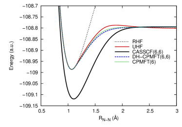
Figure 1: Potential energy curves of N₂ calculated with the cc-pVTZ basis set.

We have also performed a CPMFT calculation of the C₂ molecule with the 6-31G basis set. Near equilibrium, C₂ has significant static correlation due to near-degeneracy between the RHF occupied $\sigma_{2s}^{\star}$ and unoccupied $\sigma_{2p_{z}}$ orbitals. As the molecule is stretched, however, the $\pi_{x}$, $\pi_{y}$, $\pi_{x}^{\star}$, and $\pi_{y}^{\star}$ orbitals become degenerate, while the $\sigma_{2s}^{\star}$–$\sigma_{2p_{z}}$ interaction becomes weak. We have therefore chosen our active space to be six electrons in six orbitals for this system. In Fig. 2 we show the total energy of C₂ as a function of bond length. The CASSCF energy includes all static correlation that results from these orbital interactions (plus some dynamical correlation). Without the corresponding pairs constraint, DH-CPMFT strongly overcorrelates nearly everywhere. Adding the corresponding pairs constraint significantly reduces this overcorrelation. Near equilibrium, it gives results between UHF and CASSCF. Unfortunately, it still overcorrelates as the molecule dissociates. This is due to electron “spilling” between $\sigma_{2s}^{\star}$ and $\sigma_{2p_{z}}$ orbitals. As $R\to\infty$, only the $\pi$ orbitals should be strongly correlated; including these $\sigma$ orbitals in the active space at large internuclear separation allows them to correlate and lower the energy unphysically. If we remove two orbitals from the active space, we produce the curve marked CPMFT(4). This goes to the correct dissociation limit, but undercorrelates at equilibrium where the active space should be larger. The correct solution for this molecule involves introducing renormalized one-body potentials in CPMFT(6) that eliminate the spilling at dissociation,CPMFT2 an approach that we will discuss in a forthcoming article. While going to the right dissociation limit is important, it is perhaps less critical than getting the correct behavior near equilibrium. Note that CPMFT(4) dissociates correctly to two ROHF carbon atoms, while UHF instead dissociates to two spin-contaminated UHF carbon atoms and CASSCF(6,6) has some dynamical correlation at dissociation.

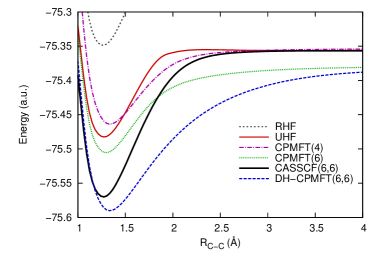
Figure 2: Potential energy curves of C₂ calculated with the 6-31G basis set.

Finally, we stress the differences between UHF and CPMFT by analyzing the dissociation of the CO₂ molecule. The ground state of CO₂ near equilibrium is a closed-shell singlet with no expected static correlation. Indeed both UHF and CPMFT reduce to the RHF solution near R_e. However, when the molecule is symmetrically stretched and the two oxygen atoms are simultaneously separated from the carbon atom, the correct dissociation limit corresponds to all three atoms in their triplet ground state. This situation cannot be handled by UHF. In CO₂ near R_e, there are six electrons associated with bond formation, three with spin-up and three with spin-down. At dissociation, UHF might assign two spin-up electrons to one oxygen atom and two spin-down electrons on the other, which puts both oxygen atoms in their triplet ground state. However, with only one electron of each spin remaining, the best UHF can do is to assign a singlet state to the carbon atom, which is clearly incorrect and not the lowest energy state. In simple words, UHF runs out of broken symmetry degrees of freedom (has only two) to model the dissociation of CO₂ (Fig. 3) and misses the correct dissociation limit by $\sim$ 20 milliHartrees. The bumps in the dissociation curves correspond to crossings of different solutions to the respective SCF equations and we have plotted the lowest energy state at each $R$. Because spin states are treated in CPMFT through an “ensemble” representation, one that yields zero spin magnetization density everywhere, the CPMFT solution for this dissociation has two half spins up and two half spins down on each of the three atoms, leading to the correct energy corresponding to the sum of ROHF atomic energies. Note that CPMFT(6) in Fig. 3 contains a one-body potential arising from an asymptotic constraint as explained in our previous publication.CPMFT2 We defer detailed discussion of the renormalization schemes used in CO₂ and applicable to C₂ within the current UHF-like context to a forthcoming publication.

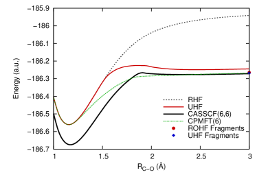
Figure 3: Potential energy curves for the double dissociation of CO₂ calculated with the 3-21G basis set.

V Conclusions

We have developed a novel scheme for performing CPMFT calculations with occupation numbers occurring in corresponding pairs. In doing so, we eliminate all chemical potentials, and the effective Fock matrices $\mathbf{F}^{\mathrm{A}}$ and $\mathbf{F}^{\mathrm{B}}$ that are to be diagonalized are of half the dimension of the double Hamiltonian matrix in the previous DH-CPMFT scheme. Thus, the computational effort in our present implementation is greatly reduced over the previous formulation of CPMFT. The corresponding pairs constraint reduces the overcorrelation of C₂ near equilibrium, and has important consequences for the dissociation of heteronuclear systems. While the corresponding pair constraint could also be imposed in the DH-CPMFT framework by addition of one Lagrange multiplier per electron pair, the current approach imposes this constraint in a simpler black-box manner.

We have shown that this version of CPMFT is closely related to UHF theory. Unlike UHF, however, CPMFT incorporates static correlation by a different mechanism. The physical density matrix $\bm{\gamma}$ has identical spin-up and spin-down blocks, whereas the auxiliary $\mathbf{A}$ and $\mathbf{B}$ density matrices, in general, break symmetry. CPMFT can correctly dissociate polyatomic molecules into ROHF atoms or fragments, whereas UHF has problems with multiple entangled electrons at multiple centers, as shown for CO₂ above. In the present formulation, CPMFT becomes a density matrix functional that can be solved by diagonalization of effective Fock matrices providing orbitals and orbital energies. We wish to emphasize one more time that as we have demonstrated, a quasiparticle picture of strong correlations with the sign of the pairing interaction reversed yields an energy expression reminiscent of UHF.

Finally, we should note that in CPMFT different auxiliary $\mathbf{A}$ and $\mathbf{B}$ density matrices can lead to solutions with degenerate energies. The key quantities determining the energy in the model are $\mathbf{P}$ and $\mathbf{K}$ and there is a many-to-one mapping between $\mathbf{A}$ and $\mathbf{B}$ on the one hand and $\mathbf{P}$ and $\mathbf{K}$ on the other. At dissociation, for example, solutions where $\mathbf{A}$ and $\mathbf{B}$ orbitals are localized and delocalized (roughly corresponding to UHF and RHF orbitals) are degenerate. The existence of additional degenerate solutions in CPMFT (compared to UHF) can lead to convergence difficulties as the active space becomes large. Efficient ways of dealing with the additional degrees of freedom provided by the auxiliary $\mathbf{A}$ and $\mathbf{B}$ matrices are currently under investigation.

VI Acknowledgments

This work was supported by NSF (Grant No. CHE-0807194), LANL Subcontract 81277-001-10, and the Welch Foundation (Grant No. C-0036). A.S. acknowledges support from ANR (Grant No. 07-BLAN-0272). We thank Carlos Jiménez-Hoyos and Jason Ellis for useful discussions and Dan Sorensen for pointing out Ref. math, .

Appendix A Properties of the CPMFT Model Two-Particle Density Matrix

The CPMFT model two-particle density matrix is

$$(\bm{\Gamma}_{\mathrm{CPMFT}})_{ij}^{kl}=\frac{1}{2}\gamma_{i}^{k}\gamma_{j}^{l}-\frac{1}{2}\gamma_{i}^{l}\gamma_{j}^{k}-\frac{1}{2}\kappa_{ij}\kappa^{kl}.$$ (39)

where $i$, $j$, $k$, and $l$ are spin-orbitals and $\bm{\gamma}$ and $\bm{\kappa}$ are the density matrix and anomalous density matrix in the spin-orbital basis (i.e, they are of dimension $2N\times 2N$, where $N$ is the size of the atomic orbital basis). In general, $\bm{\gamma}$ is Hermitian and $\bm{\kappa}$ is antisymmetric. When everything is real (which we take for simplicity; this does not affect our conclusions), the idempotent HFB quasiparticle density matrix is

$$\mathbf{R}=\begin{pmatrix}\bm{\gamma}&\bm{\kappa}\\ -\bm{\kappa}&\bm{1}-\bm{\gamma}\end{pmatrix}.$$ (40)

Idempotency tells us that

$$\bm{\gamma}\,\bm{\kappa}-\bm{\kappa}\,\bm{\gamma} =\bm{0},$$ (41a)

$$\bm{\gamma}^{2}-\bm{\kappa}^{2} =\bm{\gamma}.$$ (41b)

We recall that for closed shells,SS2002

$$\bm{\gamma} =\begin{pmatrix}\mathbf{P}&\bm{0}\\ \bm{0}&\mathbf{P}\end{pmatrix},$$ (42a)

$$\bm{\kappa} =\begin{pmatrix}\bm{0}&\mathbf{K}\\ -\mathbf{K}&\bm{0}\end{pmatrix},$$ (42b)

$$\bm{0} =\mathbf{P}\,\mathbf{K}-\mathbf{K}\,\mathbf{P},$$ (42c)

$$\mathbf{P} =\mathbf{P}^{2}+\mathbf{K}^{2}.$$ (42d)

We can define an analogous model two-particle density matrix for HFB, for which all the conditions on $\bm{\kappa}$, $\bm{\gamma}$, $\mathbf{K}$, and $\mathbf{P}$ are the same, but where

$$(\bm{\Gamma}_{\mathrm{HFB}})_{ij}^{kl}=\frac{1}{2}\gamma_{i}^{k}\gamma_{j}^{l}-\frac{1}{2}\gamma_{i}^{l}\gamma_{j}^{k}+\frac{1}{2}\kappa_{ij}\kappa^{kl}.$$ (43)

Finally, the UHF two-particle density matrix is

$$(\bm{\Gamma}_{\mathrm{UHF}})_{ij}^{kl}=\frac{1}{2}\gamma_{i}^{k}\gamma_{j}^{l}-\frac{1}{2}\gamma_{i}^{l}\gamma_{j}^{k}$$ (44)

where $\bm{\gamma}$ is idempotent. We have

$$\bm{\gamma} =\begin{pmatrix}\bm{\gamma}^{\alpha\alpha}&\bm{0}\\ \bm{0}&\bm{\gamma}^{\beta\beta}\end{pmatrix}=\begin{pmatrix}\mathbf{P}+\mathbf{M}&\bm{0}\\ \bm{0}&\mathbf{P}-\mathbf{M}\end{pmatrix},$$ (45a)

$$\mathbf{P} =\mathbf{P}^{2}+\mathbf{M}^{2},$$ (45b)

$$\mathbf{M} =\mathbf{P}\,\mathbf{M}+\mathbf{M}\,\mathbf{P}.$$ (45c)

A.1 Partial Trace of the Two-Particle Density Matrix

An important condition on the two-particle density matrix is that it traces to the one-particle density matrix. That is, we must have

$$\Gamma_{ij}^{il}=\frac{N-1}{2}\gamma_{j}^{l}.$$ (46)

We remind the reader that repeated indices are to be summed.

The partial trace condition is satisfied by the UHF two-matrix and the CPMFT model two-matrix, but not by the HFB model two-matrix:

$$\Gamma_{ij}^{il} =\frac{1}{2}\left(\gamma_{i}^{i}\gamma_{j}^{l}-\gamma_{i}^{l}\gamma_{j}^{i}\mp\kappa_{ij}\kappa^{il}\right)$$ (47a)

$$=\frac{1}{2}\left[N\gamma_{j}^{l}-(\bm{\gamma}^{2})_{j}^{l}\pm(\bm{\kappa}^{2})_{j}^{l}\right]$$ (47b)

$$=\frac{1}{2}\left[N\gamma_{j}^{l}-(\bm{\gamma}+\bm{\kappa}^{2})_{j}^{l}\pm(\bm{\kappa}^{2})_{j}^{l}\right]$$ (47c)

$$=\frac{N-1}{2}\gamma_{j}^{l}-\frac{1}{2}\left[(\bm{\kappa}^{2})_{j}^{l}\mp(\bm{\kappa}^{2})_{j}^{l}\right].$$ (47d)

Here, the top (bottom) sign in $\pm$ and $\mp$ corresponds to CPMFT (HFB), and we have used antisymmetry of $\bm{\kappa}$. Explicitly, we have

$$(\bm{\Gamma}_{\mathrm{CPMFT}})_{ij}^{il} =\frac{N-1}{2}\gamma_{j}^{l}.$$ (48a)

$$(\bm{\Gamma}_{\mathrm{HFB}})_{ij}^{il} =\frac{N-1}{2}\gamma_{j}^{l}-(\bm{\kappa}^{2})_{j}^{l}.$$ (48b)

Note that by $N$ we mean the trace of the one-particle density matrix $\bm{\gamma}$, which should be the number of particles in the system.

A.2 Particle Number Fluctuations

In order to work out particle number fluctuations, we need the expectation values of $\hat{N}$ and $\hat{N}^{2}$, with $\hat{N}$ the number operator, given as

$$\hat{N}=\delta_{pq}a_{p}^{\dagger}a_{q}.$$ (49)

We have already noted that the expectation value of $\hat{N}$ is just $\mathrm{Tr}(\bm{\gamma})$. The expectation value of $\hat{N}^{2}$ requires the two-particle density matrix:

$$\langle\hat{N}^{2}\rangle =\delta_{pq}\,\delta_{rs}\,\langle a_{p}^{\dagger}a_{q}a_{r}^{\dagger}a_{s}\rangle$$ (50a)

$$=\delta_{pq}\,\delta_{rs}\left(-\langle a_{p}^{\dagger}a_{r}^{\dagger}a_{q}a_{s}\rangle+\delta_{qr}\langle a_{p}^{\dagger}a_{s}\rangle\right)$$ (50b)

$$=\delta_{pq}\,\delta_{rs}\left(2\,\Gamma_{pr}^{qs}+\delta_{qr}\gamma_{p}^{s}\right)$$ (50c)

$$=2\,\Gamma_{pr}^{pr}+\gamma_{p}^{p}.$$ (50d)

If the two-particle density matrix obeys the partial trace condition, the particle number fluctuations are automatically zero. This is thus true of UHF and of CPMFT. However, HFB has particle number fluctuations:

$$\begin{split}\langle\hat{N}^{2}\rangle_{\mathrm{HFB}}&=(N-1)\gamma_{j}^{j}-2(\bm{\kappa}^{2})_{j}^{j}+\gamma_{j}^{j}\\ &=N^{2}-2\,\mathrm{Tr}(\bm{\kappa})^{2}\end{split}$$ (51)

implying that

$$\sigma_{N}^{2}=\langle\hat{N}^{2}\rangle-\langle\hat{N}\rangle^{2}=-2\,\mathrm{Tr}(\bm{\kappa}^{2}).$$ (52)

Note that this is positive, as it should be, since $-\bm{\kappa}^{2}~{}=\bm{\gamma}~{}-~{}\bm{\gamma}^{2}$ and occupation numbers are between 0 and 1, inclusive. In the closed-shell case, we have $\sigma_{N}^{2}=4\,\mathrm{Tr}(\mathbf{K}^{2})$.

A.3 Spin Contamination

Evaluating spin contamination is more complicated than evaluating particle number fluctuations, not least because we need an expression for $\langle\hat{S}^{2}\rangle$ for a general two-particle density matrix $\bm{\Gamma}$. We begin by noting that

$$\hat{S}^{2} =\hat{S}_{x}^{2}+\hat{S}_{y}^{2}+\hat{S}_{z}^{2}$$ (53a)

$$=\hat{S}_{z}+\hat{S}_{z}^{2}+\hat{S}_{-}\hat{S}_{+},$$ (53b)

where $\hat{S}_{\pm}$ is the spin raising/lowering operator. We are interested here in the closed-shell case (i.e. $N_{\alpha}=N_{\beta}$ with a block diagonal $\bm{\gamma}$).

In the closed-shell case, the contribution to $\langle\hat{S}^{2}\rangle$ from the first term is zero. We must evaluate the contribution from the next piece using our model two-particle density matrix. We have

$$\hat{S}_{z}^{2}=\underbrace{\sum_{i}\hat{s}_{z}(i)^{2}}_{\hat{X}_{z}}+\underbrace{\sum_{i\neq j}\hat{s}_{z}(i)\hat{s}_{z}(j)}_{\hat{Y}_{z}}.$$ (54)

The first (second) term is a one-particle (two-particle) operator. Note that we could also write

$$\hat{Y}_{z}=2\sum_{i>j}\hat{s}_{z}(i)\hat{s}_{z}(j)$$ (55)

which explains the factor of 2 that might otherwise appear to be missing below.

Evaluating the contribution to $\langle\hat{S}_{z}^{2}\rangle$ from $\hat{X}_{z}$ is straightforward, and we get just

$$\langle\hat{X}_{z}\rangle=\frac{1}{4}(N_{\alpha}+N_{\beta})=\frac{1}{2}\mathrm{Tr}(\mathbf{P}).$$ (56)

The nonzero matrix elements of $\hat{Y}_{z}$ are

$$(Y_{z})^{i_{\alpha}j_{\alpha}}_{k_{\alpha}l_{\alpha}} =\langle i_{\alpha}j_{\alpha}|\hat{Y}_{z}|k_{\alpha}l_{\alpha}\rangle=\frac{1}{2}\delta^{i}_{k}\delta^{j}_{l},$$ (57a)

$$(Y_{z})^{i_{\alpha}j_{\beta}}_{k_{\alpha}l_{\beta}} =\langle i_{\alpha}j_{\beta}|\hat{Y}_{z}|k_{\alpha}l_{\beta}\rangle=-\frac{1}{2}\delta^{i}_{k}\delta^{j}_{l},$$ (57b)

$$(Y_{z})^{i_{\beta}j_{\alpha}}_{k_{\beta}l_{\alpha}} =\langle i_{\beta}j_{\alpha}|\hat{Y}_{z}|k_{\beta}l_{\alpha}\rangle=-\frac{1}{2}\delta^{i}_{k}\delta^{j}_{l},$$ (57c)

$$(Y_{z})^{i_{\beta}j_{\beta}}_{k_{\beta}l_{\beta}} =\langle i_{\beta}j_{\beta}|\hat{Y}_{z}|k_{\beta}l_{\beta}\rangle=\frac{1}{2}\delta^{i}_{k}\delta^{j}_{l}.$$ (57d)

Here, we are working in an orthornomal basis set.

The relevant components of the CPMFT and HFB two-particle density matrices are

$$\Gamma_{i_{\alpha}j_{\alpha}}^{k_{\alpha}l_{\alpha}} =\frac{1}{2}\left(\gamma_{i_{\alpha}}^{k_{\alpha}}\gamma_{j_{\alpha}}^{l_{\alpha}}-\gamma_{i_{\alpha}}^{l_{\alpha}}\gamma_{j_{\alpha}}^{k_{\alpha}}\right),$$ (58a)

$$\Gamma_{i_{\alpha}j_{\beta}}^{k_{\alpha}l_{\beta}} =\frac{1}{2}\left(\gamma_{i_{\alpha}}^{k_{\alpha}}\gamma_{j_{\beta}}^{l_{\beta}}\mp\kappa_{i_{\alpha}j_{\beta}}\kappa^{k_{\alpha}l_{\beta}}\right),$$ (58b)

$$\Gamma_{i_{\beta}j_{\alpha}}^{k_{\beta}l_{\alpha}} =\frac{1}{2}\left(\gamma_{i_{\beta}}^{k_{\beta}}\gamma_{j_{\alpha}}^{l_{\alpha}}\mp\kappa_{i_{\beta}j_{\alpha}}\kappa^{k_{\beta}l_{\alpha}}\right),$$ (58c)

$$\Gamma_{i_{\beta}j_{\beta}}^{k_{\beta}l_{\beta}} =\frac{1}{2}\left(\gamma_{i_{\beta}}^{k_{\beta}}\gamma_{j_{\beta}}^{l_{\beta}}-\gamma_{i_{\beta}}^{l_{\beta}}\gamma_{j_{\beta}}^{k_{\beta}}\right),$$ (58d)

where the top (bottom) sign corresponds to CPMFT (HFB).

Contracting the density matrices with the matrix elements, we get

$$\langle\hat{Y}_{z}\rangle=\left(\frac{N_{\alpha}-N_{\beta}}{2}\right)^{2}-\frac{1}{4}\mathrm{Tr}(\bm{\gamma}_{\alpha\alpha}^{2}+\bm{\gamma}_{\beta\beta}^{2}\mp\bm{\kappa}_{\alpha\beta}^{2}\mp\bm{\kappa}_{\beta\alpha}^{2})$$ (59)

where we have used antisymmetry of $\bm{\kappa}$. Working in our closed-shell case, this reduces to

$$\langle\hat{Y}_{z}\rangle=-\frac{1}{2}\mathrm{Tr}(\mathbf{P}^{2}\mp\mathbf{K}^{2}).$$ (60)

In total, then, we find that $\langle\hat{S}_{z}^{2}\rangle$ in CPMFT and HFB is given by

$$\langle\hat{S}_{z}^{2}\rangle =\frac{1}{2}\mathrm{Tr}(\mathbf{P}-\mathbf{P}^{2}\pm\mathbf{K}^{2})$$ (61a)

$$=\frac{1}{2}\mathrm{Tr}(\mathbf{K}^{2}\pm\mathbf{K}^{2}).$$ (61b)

Thus, we end up with

$$\langle\hat{S}_{z}^{2}\rangle_{\mathrm{HFB}} =0,$$ (62a)

$$\langle\hat{S}_{z}^{2}\rangle_{\mathrm{CPMFT}} =\mathrm{Tr}(\mathbf{K}^{2}).$$ (62b)

The contribution to $\langle\hat{S}^{2}\rangle$ from $\hat{S}_{-}\hat{S}_{+}$ must also be evaluated using the model two-particle density matrix. Expanding this operator in terms of contributions from individual electrons, we have

$$\hat{S}_{-}\,\hat{S}_{+}=\underbrace{\sum_{i}\hat{s}_{-}(i)\hat{s}_{+}(i)}_{\hat{X}}+\underbrace{\sum_{i\neq j}\hat{s}_{-}(i)\hat{s}_{+}(j)}_{\hat{Y}}.$$ (63)

The first term is the one-particle operator $\hat{X}$, and the second is the two-particle operator $\hat{Y}$.

Since $\hat{X}$ does nothing to down-spin electrons but annihilates up-spin electrons, we clearly have

$$\langle\hat{X}\rangle=N_{\beta}=\mathrm{Tr}(\mathbf{P}).$$ (64)

To take the expectation value of $\hat{Y}$, it proves useful to symmetrize it so that it acts the same on the two electrons. Since operators acting on different electrons commute, we have

$$\hat{Y} =\sum_{i\neq j}\hat{s}_{-}(i)\hat{s}_{+}(j)$$ (65a)

$$=\frac{1}{2}\sum_{i\neq j}\left(\hat{s}_{-}(i)\hat{s}_{+}(j)+\hat{s}_{+}(i)\hat{s}_{-}(j)\right)$$ (65b)

$$=\sum_{i>j}\left(\hat{s}_{-}(i)\hat{s}_{+}(j)+\hat{s}_{+}(i)\hat{s}_{-}(j)\right).$$ (65c)

The only nonzero matrix elements of $\hat{Y}$ are

$$Y^{i_{\beta}j_{\alpha}}_{k_{\alpha}l_{\beta}} =\langle i_{\beta}j_{\alpha}|\hat{Y}|k_{\alpha}l_{\beta}\rangle=\delta^{i}_{k}\delta^{j}_{l},$$ (66a)

$$Y^{i_{\alpha}j_{\beta}}_{k_{\beta}l_{\alpha}} =\langle i_{\alpha}j_{\beta}|\hat{Y}|k_{\beta}l_{\alpha}\rangle=\delta^{i}_{k}\delta^{j}_{l}.$$ (66b)

The relevant spin components of the CPMFT and HFB model two-particle density matrix are

$$\Gamma_{i_{\alpha}j_{\beta}}^{k_{\beta}l_{\alpha}} =\frac{1}{2}\left(-\gamma_{i_{\alpha}}^{l_{\alpha}}\gamma_{j_{\beta}}^{k_{\beta}}\mp\kappa_{i_{\alpha}j_{\beta}}\kappa^{k_{\beta}l_{\alpha}}\right),$$ (67a)

$$\Gamma_{i_{\beta}j_{\alpha}}^{k_{\alpha}l_{\beta}} =\frac{1}{2}\left(-\gamma_{i_{\beta}}^{l_{\beta}}\gamma_{j_{\alpha}}^{k_{\alpha}}\mp\kappa_{i_{\beta}j_{\alpha}}\kappa^{k_{\alpha}l_{\beta}}\right),$$ (67b)

where again CPMFT (HFB) corresponds to the top (bottom) sign.

Contracting the two-particle density matrix with the matrix elements gives us

$$\langle\hat{Y}\rangle=-\mathrm{Tr}(\bm{\gamma}_{\alpha\alpha}\bm{\gamma}_{\beta\beta}\mp\bm{\kappa}_{\alpha\beta}\bm{\kappa}_{\alpha\beta}).$$ (68)

In the closed-shell case, using the results in Eqn. (42), this becomes

$$\langle\hat{Y}\rangle=-\mathrm{Tr}(\mathbf{P}^{2}\mp\mathbf{K}^{2}).$$ (69)

Then the expectation value of $\hat{S}_{-}\hat{S}_{+}$ is given by

$$\langle\hat{S}_{-}\hat{S}_{+}\rangle =\mathrm{Tr}(\mathbf{P}-\mathbf{P}^{2}\mp\mathbf{K}^{2})$$ (70a)

$$=\mathrm{Tr}(\mathbf{K}^{2}\mp\mathbf{K}^{2}).$$ (70b)

We therefore have

$$\langle\hat{S}_{-}\hat{S}_{+}\rangle_{\mathrm{HFB}} =2\mathrm{Tr}(\mathbf{K}^{2}),$$ (71a)

$$\langle\hat{S}_{-}\hat{S}_{+}\rangle_{\mathrm{CPMFT}} =0.$$ (71b)

Combining Eqns. (62) and (71) gives us the total spin contamination in HFB and in CPMFT:

$$\langle\hat{S}^{2}\rangle_{\mathrm{HFB}} =2\mathrm{Tr}(\mathbf{K}^{2}),$$ (72a)

$$\langle\hat{S}^{2}\rangle_{\mathrm{CPMFT}} =\mathrm{Tr}(\mathbf{K}^{2}),$$ (72b)

For UHF in cases in which there is strong correlation, we have the familiar formula

$$\langle\hat{S}^{2}\rangle=s(s+1)+N_{\beta}-\mathrm{Tr}(\bm{\gamma}_{\alpha\alpha}\,\bm{\gamma}_{\beta\beta}).$$ (73)

For the closed-shell case, using the results in Eqn. (45), we have

$$\langle\hat{S}^{2}\rangle =\mathrm{Tr}[\mathbf{P}-(\mathbf{P}+\mathbf{M})(\mathbf{P}-\mathbf{M})]$$ (74)

$$=\mathrm{Tr}(\mathbf{P}-\mathbf{P}^{2}+\mathbf{M}^{2})$$

$$=2\,\mathrm{Tr}(\mathbf{M}^{2}).$$

References

- (1) T. Tsuchimochi and G. E. Scuseria, J. Chem. Phys. 131, 121102 (2009).
- (2) G. E. Scuseria and T. Tsuchimochi, J. Chem. Phys. 131, 164119 (2009).
- (3) T. Tsuchimochi, G. E. Scuseria, and A. Savin, J. Chem. Phys. 132, 024111 (2010).
- (4) J-P. Blaizot and G. Ripka, “Quantum Theory of Finite Systems” (The MIT Press, Massachusetts, 1986).
- (5) V. N. Staroverov and G. E. Scuseria, J. Chem. Phys. 117, 11107 (2002).
- (6) K. Takatsuka, T. Fueno, and K. Yamaguchi, Theoret. Chim. Acta 48, 175 (1978).
- (7) V. N. Staroverov and E. R. Davidson, Chem. Phys. Lett. 330, 161 (2000).
- (8) I. Mayer, Chem. Phys. Lett. 440, 357 (2007).
- (9) W. Kutzelnigg and D. Mukherjee, J. Chem. Phys. 110, 2800 (1999).
- (10) G. Csnyi and T. A. Arias, Phys. Rev. B 61, 7348 (2000).
- (11) J. A. Pople and R. K. Nesbet, J. Chem. Phys. 22, 571 (1954).
- (12) Note that UHF subtracts from the closed shell energy while CPMFT subtracts . However, these are the same if the basis functions and the anomalous density matrix are real, as they generally are.
- (13) H. Fukutome, Int. J. Quantum Chem. 20, 955 (1981).
- (14) A. T. Amos and G. G. Hall, Proc. Roy. Soc. (London) A263, 483 (1961).
- (15) J. E. Harriman, J. Chem. Phys. 40, 2827 (1964).
- (16) V. Rabanovich, Linear Algebra Appl. 390, 137 (2004).
- (17) More precisely, the eigenvalues of for idempotent and are 0, , , or a corresponding pair .
- (18) M. J. Frisch, G. W. Trucks, H. B. Schlegel, et al., Gaussian Development Version, Revion G.01, Gaussian, Inc., Wallingford CT, 2007.