Rational Orbits around Charged Black Holes

Abstract

We show that all eccentric timelike orbits in Reissner-Nordström spacetime can be classified using a taxonomy that draws upon an isomorphism between periodic orbits and the set of rational numbers. By virtue of the fact that the rationals are dense, the taxonomy can be used to approximate aperiodic orbits with periodic orbits. This may help reduce computational overhead for calculations in gravitational wave astronomy. Our dynamical systems approach enables us to study orbits for both charged and uncharged particles in spite of the fact that charged particle orbits around a charged black hole do not admit a simple one-dimensional effective potential description. Finally, we show that comparing periodic orbits in the RN and Schwarzschild geometries enables us to distinguish charged and uncharged spacetimes by looking only at the orbital dynamics.

I Introduction

Black holes are useful large-scale laboratories for testing general relativity in strong gravitational fields. While directly observing black holes proves difficult because they emit no electromagnetic radiation, black hole pairs can be detected via the gravitational radiation they may emit. The terrestrial network of interferometric gravitational wave detectors and the proposed space-based detector LISA (Laser Interferometer Space Antenna), are expected to detect gravitational radiation and launch an era of gravitational wave astronomy that would make use of direct observations of black holes.

Because gravitational waves are shaped by the motion of massive celestial objects, extracting astrophysically meaningful information from them requires a comprehensive theoretical understanding of the sources’ underlying dynamics flanagan ; glampedakis2 ; drasco1 ; drasco2 ; drasco3 ; lang . For example, one popular processing method, matched filtering, makes use of a template signal, generated using theoretical predictions, to find signals in noisy detector output glampedakis ; grishchuk . Template signal generation is an example of the type of computationally expensive process encountered in gravitational wave astronomy when studying aperiodic orbits in the strong-field regime.

A method for approximating aperiodic orbits with periodic orbits, which could cut down significantly on computational expenses, was introduced in an earlier paper levin . The approximation method takes the form of a taxonomy that assigns to each periodic orbit a rational number. By virtue of the fact that the rationals are dense, the taxonomy can be used to approximate aperiodic orbits with periodic orbits to arbitrary precision. Because periodic orbits might have Fourier series that converge more rapidly than those of aperiodic orbits, and because for periodic orbits the evolution of a geometry’s conserved quantities may be interdependent, calculations pertaining to periodic orbits might be less computationally intensive than those for aperiodic orbits levin .

The taxonomy was applied to the Kerr geometry in levin and levin_el and to black hole pairs in levin_d1 and levin_d2 . Here, we will extend the approach to the Reissner-Nordström (RN) solution to the Einstein field equations, which describes the gravitational field of a static, non-rotating, electrically charged, spherically symmetric body carroll . Studying a geometry of this type is less astrophysically motivated than studying its electrically neutral counterpart. Were it to form in spite of the fact that the electromagnetic repulsion in compressing an electrically charged mass is greater by about 40 orders of magnitude than the gravitational attraction, it would neutralize its own electric charge if enough opposite charge were available. Nonetheless, in the spirit of being prepared for the unexpected, and in support of the ambitious gravitational wave experiments coming online, we will not presumptively exclude any possible sources. Were gravitational waves from a charged black hole candidate detected experimentally, a thorough understanding of the RN orbits could help identify their source.

At the other extreme, microscopic black holes that might form in accelerator experiments may be charged. A pair of black holes that scatter and then evaporate might be described by a scattering amplitude that is a sum over these classical paths. The solutions we describe might find application in particle physics as well as astrophysics.

Both Kerr and RN orbits bear many qualitative similarities to orbits in Schwarzschild spacetime, including “zoom-whirl” behavior barack ; glampedakis , in which the test particle zooms away from the central mass quasielliptically to successive apastra separated by nearly circular whirls. It is this behavior which the taxonomy exploits. As was the case for Kerr orbits before this taxonomy was introduced, no unifying framework for making general claims about orbits has been applied to the RN spacetime before.

II Reissner-Nordström Effective Potential

We use the effective potential formulation of the RN spacetime to calculate various interesting dynamical properties of the geometry. In an appendix we detail the Hamiltonian formulation that is used to generate the orbits pictured throughout the paper. We begin with the RN metric,

$$g_{\mu\nu}=\left(\begin{array}[]{cccc}-\Delta&&&\\ &\Delta^{-1}&&\\ &&r^{2}&\\ &&&r^{2}\sin^{2}\theta\end{array}\right),$$ (1)

where the horizon function $\Delta$ is

$$\Delta=1-\frac{2}{r}+\frac{Q^{2}}{r^{2}}.$$ (2)

We have assumed that the central magnetic charge is zero, which would otherwise change the horizon function’s third term to $(Q^{2}+P^{2})/r^{2}$ . We use geometrized units and measure $r$ and the central charge $Q$ in units of ${M}$.

A first constant of motion is always

$$g_{\mu\nu}\frac{dx^{\mu}}{d\tau}\frac{dx^{\nu}}{d\tau}=\kappa,\$$ (3)

$$\kappa=\bigg{\{}\begin{array}[]{l l}-1&\quad\mbox{for timelike geodesics}\\ 0&\quad\mbox{for null geodesics}\\ \end{array}\ .$$

Explicitly, for timelike orbits, this gives

$$-\Delta\,\dot{t}^{2}+\frac{1}{\Delta}\,\dot{r}^{2}+r^{2}\,\dot{\theta}^{2}+r^{2}\sin^{2}\theta\,\dot{\varphi}^{2}=-1,$$ (4)

where an overdot indicates differentiation with respect to an affine parameter $\tau$.

To derive expressions for the conserved quantities we write the Lagrangian for a charged particle, in which the final term is derived using the fact that the only nonvanishing component of the vector potential $A_{\mu}$ is $A_{0}$ chandra :

$$\mathcal{L}=\frac{1}{2}\big{(}-\Delta\,\dot{t}^{2}+\frac{1}{\Delta}\,\dot{r}^{2}+r^{2}\,\dot{\theta}^{2}+r^{2}\sin^{2}\theta\,\dot{\varphi}^{2}\big{)}-\frac{QQ_{*}}{r}\dot{t}.$$ (5)

$Q_{*}$ is the charge per unit mass of the test particle. Geodesics in the RN geometry are constrained to a plane. Since the geometry is spherically symmetric, we can set $\theta=\pi/2$ and $\dot{\theta}=0$ so that every geodesic is equatorial.

Using

$$\frac{d}{d\tau}\left(\frac{\partial\mathcal{L}}{\partial\dot{q}}\right)-\frac{d\mathcal{L}}{dq}=0,$$ (6)

yields the constants of motion:

$$p_{t}=-\Delta\dot{t}-\frac{QQ_{*}}{r}=-E\hskip 36.135ptp_{\varphi}=r^{2}\dot{\varphi}=L.$$ (7)

Applying (7) to (4) and simplifying gives us

$$\frac{1}{2}\dot{r}^{2}+V_{\textrm{eff}}=\mathcal{E}_{\textrm{eff}},$$ (8)

where

$$V_{\textrm{eff}} = \left(-1+EQQ_{*}\right)\frac{1}{r}+\left(\frac{L^{2}+Q^{2}-Q^{2}Q_{*}^{2}}{2}\right)\frac{1}{r^{2}}+\left(-L^{2}\right)\frac{1}{r^{3}}+\left(\frac{Q^{2}L^{2}}{2}\right)\frac{1}{r^{4}}$$ (9)

$$\mathcal{E}_{\textrm{eff}} = \frac{E^{2}-1}{2}.$$ (10)

Due to the geometry’s spherical symmetry, the effective potential is one-dimensional – just as in the Schwarzschild case – but with one caveat: the test particle’s charge $Q_{*}$ is coupled to the energy E. This prohibits us from writing $V_{\textrm{eff}}$ in a form that is independent of energy without also writing $\mathcal{E}_{\textrm{eff}}$ in a form that is not constant. First we will consider the case when $Q_{*}=0$ so that we can define a true one-dimensional effective potential. Applying this condition to (9) gives us the effective RN potential for an uncharged particle:

$$V_{\textrm{eff}} =-\frac{1}{r}+\frac{L^{2}+Q^{2}}{2r^{2}}-\frac{L^{2}}{r^{3}}+\frac{Q^{2}L^{2}}{2r^{4}}$$

$$=-\frac{1}{r}+\frac{\Delta L^{2}}{2r^{2}}+\frac{Q^{2}}{2r^{2}}$$

$$=\frac{\Delta L^{2}}{2r^{2}}+\frac{\Delta-1}{2}\quad.$$ (11)

We return to the charged test particle in §IV.

III Uncharged Particle Orbits in RN Spacetime

III.1 Bounds on Q

For an uncharged particle, the RN geometry is qualitatively similar outside the horizon to the Schwarzschild geometry chandra . But because the RN $V_{\textrm{eff}}$ is larger than the Schwarzschild $V_{\textrm{eff}}$ by a factor of $\frac{Q^{2}}{2r^{2}}+\frac{Q^{2}L^{2}}{2r^{4}}$, a thorough quantitative analysis is necessary to understand the orbital dynamics. Our goal in this section is to determine the bounds on $L$ and $Q$ that yield periodic orbits.

Determining bounds on $Q$ is simple: owing to the RN geometry’s peculiar horizon structure, only certain values of $Q$ are realistic carroll . The null hypersurfaces are given by

$$g^{rr}=\Delta(r)=1-\frac{2}{r}+\frac{Q^{2}}{r^{2}}=0,$$ (12)

which when solved for $r$ gives us the horizons:

$$r_{\pm}=1\pm\sqrt{1-Q^{2}}.$$ (13)

When $Q^{2}>1$, the geometry is a naked singularity. The condition $Q^{2}=1$ describes an extremal RN black hole, which is highly unstable due to the fact that adding any mass at all makes it an undercritically charged black hole. This leaves the undercritically charged geometry ($Q^{2}<1$) as the most realistic scenario. Because $Q$ only appears in the potential as $Q^{2}$, the undercritically charged case is equivalently given by $-1<Q<1$.

$Q$ affects the shape of the potential as shown in Figure 1. Note that the $Q=0$ case (solid) is simply the Schwarzschild effective potential. When comparing the RN potential to the Schwarzschild potential, we see that the factor of $+Q^{2}/2$ in the $r^{-2}$ term is the reason for the heightened peak and that the $r^{-4}$ term makes the potential blow up at zero.

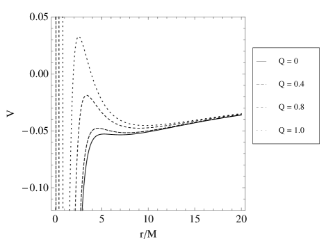
Figure 1: $V_{\textrm{eff}}$ for $Q=0$, $0.4$, $0.8$, and $1$, from bottom to top

The Schwarzschild $V_{\textrm{eff}}$ has at most two extrema. Because the RN $V_{\textrm{eff}}$ is a quartic, it can have three extrema. This opens up the possibility of three circular orbits – two stable and one unstable – outside the horizon. The existence of two stable circular orbits would imply that there are two regions in which we can find bounded orbits. There would be two stable circular orbits if both minima were to lie outside the outer horizon, $r_{+}$. Figure 2 depicts the Schwarzschild and RN potentials for $L=3.2$. The dashed potential is the Schwarzschild $V_{\textrm{eff}}$ and the Schwarzschild horizon is given by the dashed vertical line ($r=2$). The RN $V_{\textrm{eff}}$ and external horizon are solid. For this choice of $L$ and $Q$ there are only two extrema outside the RN horizon, one stable and one unstable. We want to determine if there are any $L$ and $Q$ for which the external horizon is closer to the singularity than the inner minimum of the potential. This would yield two stable circular orbits.

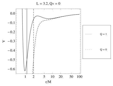
Figure 2: The RN and Schwarzschild potentials with horizons for each and a non-physical internal horizon (dotted) that represents a scenario in which there are multiple stable circular orbits

Our first step is to find the radii $r_{c}$ at which the effective potential has stationary points, given by

$$\frac{dV_{\textrm{eff}}}{dr}=\frac{1}{r^{2}}-\frac{Q^{2}+L^{2}}{r^{3}}+\frac{3L^{2}}{r^{4}}-\frac{2Q^{2}L^{2}}{r^{5}}=0.$$ (14)

We rewrite this as

$$r_{c}^{3}-(Q^{2}+L^{2})r_{c}^{2}+3L^{2}r_{c}-2Q^{2}L^{2}=0$$ (15)

and take its discriminant to get

$$D=-108L^{6}+9L^{8}+126L^{6}Q^{2}-8L^{8}Q^{2}+9L^{4}Q^{4}-24L^{6}Q^{4}-24L^{4}Q^{6}-8L^{2}Q^{8}.$$ (16)

When $D>0$, $\frac{\partial V_{\textrm{eff}}}{\partial r}$ has 3 distinct, real roots, and $V_{\textrm{eff}}$ has 3 extrema. If the condition $D>0$ is ever true when the $r_{c}$ are all $>\,r_{+}$, the external horizon, we will have two stable circular orbits. The solutions of Equation (15) for $r_{c}$ do not provide much insight, so we will not reproduce them here. Instead we represent the solutions graphically.

The disjointedness of the regions in parameter space that satisfy each of the above conditions is demonstrated in Figure 3. The regions with horizontal hatching are those in which $D>0$ and the regions with vertical hatching are where the smallest circular orbit $r_{c}>r_{+}$. Note that the vertically hatched region does not presume the existence of three extrema. There is no overlap between the two regions when $-1<Q<1$ and $Q_{*}=0$, so in these conditions we never see three extrema outside the event horizon. Therefore, there is always at most one stable circular orbit. This clarifies the region of the effective potential in which we find periodic orbits and confirms that for $Q_{*}=0$, there is always at most one stable circular orbit.

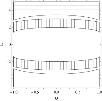
Figure 3: Regions in which the potential has three extrema (horizontal hatching) and those in which the smallest extremum is outside the horizon. (vertical hatching)

III.2 Bounds on L

We have established that in the undercritically-charged RN geometry for a neutral particle, for any L there is at most one stable circular orbit. Figure 4 depicts the potential for various $L$ with $Q$ fixed.

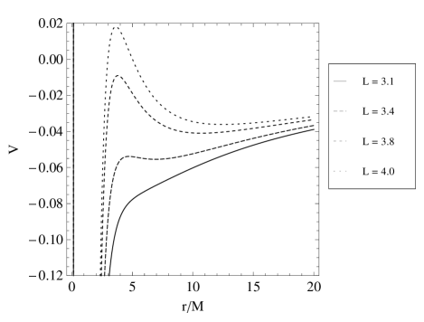
Figure 4: $V_{\textrm{eff}}$ for $L=3.1$, $3.4$, $3.8$, and $4.0$, from bottom to top, with $Q$ fixed.

We will now determine the bounds in the undercritically-charged RN geometry that specify the region in which we find most zoom-whirl behavior levin ,

$$L_{\rm ISCO}<L<L_{\rm IBCO},$$ (17)

where ISCO stands for “Innermost Stable Circular Orbit” and IBCO for “Innermost Bound Circular Orbit”. $L_{\textrm{ISCO}}$ is the lowest value of $L$ for which the potential has a local minimum, and therefore marks the first appearance of a stable circular orbit. For $L<L_{\textrm{ISCO}}$, all orbits will plunge into the black hole, so $L_{\textrm{ISCO}}$ sets the lower limit on bound orbits. $L_{\textrm{IBCO}}$ marks the first appearance of an unstable circular orbit that is energetically bound. It sets the upper limit only in the sense that we expect to see the most zoom-whirl behavior in the strong-field when such an unstable bound orbit comes into play levin . Orbits will whirl more as they roll up the potential towards the unstable bound circular orbit.

To derive expressions for $L_{\textrm{ISCO}}$ and $L_{\textrm{IBCO}}$ we start with the conditions for circular orbits. Equation (8), written with $V_{\textrm{eff}}$ as it appears in Equation (II), is

$$\frac{1}{2}\dot{r}^{2}+\frac{\Delta L^{2}}{2r^{2}}+\frac{\Delta-1}{2}=\mathcal{E}_{\textrm{eff}},$$ (18)

The two conditions for circular orbits are $\dot{r}=0$ and $\ddot{r}=0$, which imply that

$$V_{\rm eff} = \frac{E^{2}-1}{2}$$

$$\frac{\partial V_{\rm eff}}{\partial r} = 0.$$ (19)

The first condition, when solved for $L^{2}$, gives us

$$L^{2}=\left(\frac{E^{2}}{\Delta}-1\right)r^{2}.$$ (20)

We may rewrite $\frac{\partial V}{\partial r}$ as

$$\frac{\partial V_{\textrm{eff}}}{\partial r} = \Delta\left(\frac{-L^{2}}{r^{3}}+\frac{\Delta^{\prime}}{\Delta}\left(\frac{L^{2}}{2r^{2}}+\frac{1}{2}\right)\right)$$ (21)

$$= \Delta\left(\frac{-L^{2}}{r^{3}}+\frac{\Delta^{\prime}}{\Delta^{2}}\left(V_{\textrm{eff}}+\frac{1}{2}\right)\right)$$ (22)

where

$$\Delta^{\prime}=\frac{d\Delta}{dr}=\frac{2}{r^{2}}-\frac{2Q^{2}}{r^{3}}.$$ (23)

Applying the conditions for circular orbits in Equation (19) gives us

$$\frac{\partial V_{\textrm{eff}}}{\partial r} = \Delta\left(\frac{-L^{2}}{r^{3}}+\frac{\Delta^{\prime}}{\Delta^{2}}\left(\frac{E^{2}}{2}\right)\right)=0\quad$$ (24)

Solving for $L^{2}$ gives us

$$L^{2}=r^{3}\frac{\Delta^{\prime}}{\Delta^{2}}\left(\frac{E^{2}}{2}\right).$$ (25)

Equating Equations (20) and (25) and solving for $E^{2}$ gives

$$E_{c}^{2}(r_{c},Q)=\frac{2\Delta^{2}}{2\Delta-r\Delta^{\prime}}.$$ (26)

Putting Equation (26) into Equation (20) and solving for $L^{2}$ yields

$$L_{c}^{2}(r_{c},Q)=r^{2}\left(\frac{r\Delta^{\prime}}{2\Delta-r\Delta^{\prime}}\right).$$ (27)

With $L_{c}$ and $E_{c}$ in hand, each of which is depicted in Figure 5, our next task is to calculate $r_{\textrm{IBCO}}$ and $r_{\textrm{ISCO}}$. Because at infinity the potential is $0$, $r_{\textrm{IBCO}}$ is simply the radius of unstable circular orbit $r_{c}$ such that $V_{\textrm{eff}}(r_{c})=0$. We first solve

$$V_{\textrm{eff}}=0=\frac{\Delta L^{2}}{2r^{2}}+\frac{\Delta-1}{2}\\$$ (28)

for $L^{2}$ to obtain

$$L_{V=0}^{2}=\frac{1-\Delta}{\Delta}r^{2}.$$ (29)

Setting this equal to $L_{c}^{2}$ gives us an expression we may use to find $r_{\textrm{IBCO}}$:

$$L_{c}^{2} = L_{V=0}^{2}$$ (30)

$$r^{2}\left(\frac{r\Delta^{\prime}}{2\Delta-r\Delta^{\prime}}\right) = \left(\frac{1-\Delta}{\Delta}\right)r^{2}$$ (31)

$$0 = 2\Delta-r\Delta^{\prime}-2\Delta^{2}.$$ (32)

Solving this for r gives us

$$r_{\textrm{IBCO}} = \frac{1}{6}\left(8-\frac{8\cdot 2^{1/3}(-4+3Q^{2})}{G(Q)}+2^{2/3}G(Q)\right)$$ (33)

$$G(Q) = \sqrt[3]{128-144Q^{2}+27Q^{4}+3\sqrt{-96Q^{6}+81Q^{8}}}.$$

$L_{\textrm{IBCO}}$ is then $L_{c}$ with $r_{\textrm{IBCO}}$ in place of $r$:

$$L_{\textrm{IBCO}}^{2}=\frac{-Q^{2}r_{\textrm{IBCO}}^{2}+r_{\textrm{IBCO}}^{3}}{2Q^{2}-3r_{\textrm{IBCO}}+r_{\textrm{IBCO}}^{2}}.$$ (34)

We determine $r_{\textrm{ISCO}}$ by taking $V_{\textrm{eff}}^{\prime\prime}=0$ (differentiated with respect to $r$), or

$$\frac{\partial^{2}V_{\textrm{eff}}}{\partial r^{2}}=\frac{3L^{2}\Delta}{r^{4}}-\frac{2L^{2}\Delta^{\prime}}{r^{3}}+\frac{(L^{2}+r^{2})\Delta^{\prime\prime}}{2r^{2}}=0,$$ (35)

where

$$\Delta^{\prime\prime}=-\frac{4}{r^{3}}+\frac{6Q^{2}}{r^{4}}.$$ (36)

Solving for $L^{2}$ gives us

$$L_{\textrm{V}^{\prime\prime}\textrm{=0}}^{2}=\frac{r^{4}\Delta^{\prime\prime}}{4\Delta^{\prime}r-6\Delta-\Delta^{\prime\prime}r^{2}}$$ (37)

Setting $L_{\textrm{V}^{\prime\prime}\textrm{=0}}^{2}$ equal to $L_{c}^{2}$ and solving for $r$ gives us

$$r_{\textrm{ISCO}} = 2+\frac{4-3Q^{2}}{H(Q)}+H(Q)$$ (38)

$$H(Q) = \sqrt[3]{8-9Q^{2}+2Q^{4}+\sqrt{5Q^{4}-9Q^{6}+4Q^{8}}},$$

which when plugged into $L_{c}$ gives us

$$L_{\textrm{ISCO}}^{2}=\frac{-Q^{2}r_{\textrm{ISCO}}^{2}+r_{\textrm{ISCO}}^{3}}{2Q^{2}-3r_{\textrm{ISCO}}+r_{\textrm{ISCO}}^{2}}.$$ (39)

$r_{\textrm{IBCO}}$ and $r_{\textrm{ISCO}}$ are plotted in Figure  6.

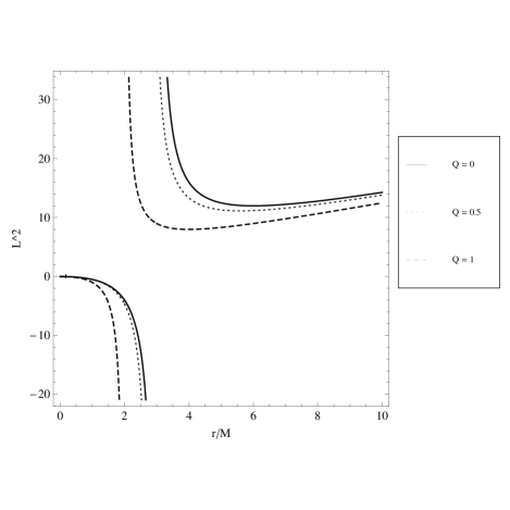
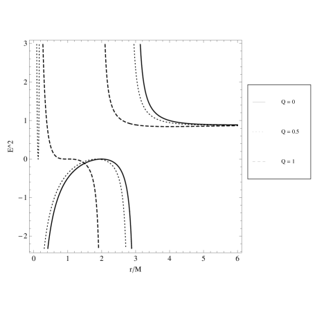
Figure 5: $L_{c}^{2}$ and $E_{c}^{2}$ as functions of $r$ for $Q=1$, $Q=0.5$, and $Q=0$.

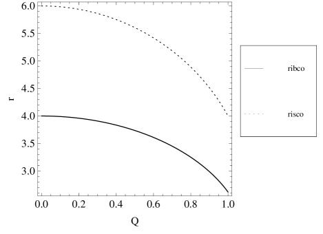
Figure 6: $r_{\textrm{IBCO}}$ (solid) and $r_{\textrm{ISCO}}$ (dotted) as a function of $Q$

We can confirm that the presence of three stationary points in the potential is tied to $L_{\textrm{ISCO}}$ by checking whether the regions in parameter space $D>0$ and $L^{2}>L_{\textrm{ISCO}}^{2}$ coincide. Figure 7 shows that this is the case within our bounds for $Q$.

Having established bounds on $Q$ and $L$ for the $Q_{*}=0$ case, we can taxonomize all zoom-whirl behavior in the strong field bounded by $L_{\textrm{ISCO}}<L<L_{\textrm{IBCO}}$, as we show in §V. First, we briefly discuss homoclinic orbits and then the $Q_{*}\neq 0$ case.

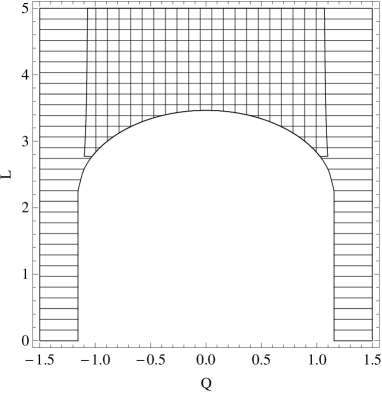
Figure 7: Regions in which $L^{2}>L_{\textrm{ISCO}}^{2}$ (horizontal hatching) and where the discriminant $D>0$ (vertical hatching). When we impose the bound $-1<Q<1$ the two regions are equivalent, which demonstrates that only when $L^{2}>L_{\textrm{ISCO}}^{2}$ does the potential have three extrema.

III.3 Homoclinic Orbits

For any $L$ such that $L_{\textrm{ISCO}}<L<L_{\textrm{IBCO}}$, there is an unstable circular orbit called a homoclinic orbit. The homoclinic orbit is the separatrix between orbits that plunge to the horizon and those that do not levin_h1 . It provides us with the infinite-whirl limit and is therefore an important landmark in the orbital landscape. Because homoclinic orbits are central to strong-field dynamics levin ; levin_h1 ; levin_h2 ; levin_d2 , we include the orbital plot of a homoclinic orbit for an uncharged particle in RN spacetime in Figure 8.

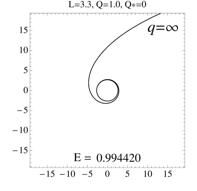
Figure 8: A homoclinic orbit for $Q=1.0$, $Q_{*}=0$, $L=3.3$

IV Charged Particle Orbits in RN Spacetime

Having discussed the uncharged test particle scenario, we will now move on to orbits in which the particle has nonzero charge. While the $Q_{*}\neq 0$ effective potential (Equation (9)) depends on both $L$ and $E$, it still only depends on one dynamical variable, $r$. Because there is no dependence on $\theta$, $\varphi$ or $t$, every bound orbit has fixed apastra and periastra that are functions of $Q$, $L$, and $E$, so we still find periodicity. As such, we can make use of this potential to study orbits for charged particles. However, the method for finding periodic orbits is more complicated than in the $Q_{*}=0$ case, because given a particular effective potential we may no longer choose $\mathcal{E}_{\textrm{eff}}$ so as to produce a periodic orbit, because the potential is coupled to $E$.

Figure 9: $V_{\textrm{eff}}$ for $Q_{*}=\{0,0.1,0.2,0.3,1.0\}$ from bottom to top, with $\mathcal{E}_{\textrm{eff}}=\frac{-1+E^{2}}{2}=0.99$, $Q=1$, $L=3.5$

IV.1 Identifying Regions with Bounded Orbits

Because we are considering only test particles we assume that the particle mass $m$ is $<<M$, which implies that $Q_{*}<(m/M)<1$. As before, we first want to determine whether the potential ever has three extrema outside the horizon, which we do by determining if it is ever simultaneously the case that the discriminant of $\frac{\partial V_{\textrm{eff}}}{\partial r}$ is positive – which means that there are three extrema – and that the smallest of the extrema is at a radius $>r_{+}$. The region of parameter space in which each condition is true is depicted in Figures 10 and 11, respectively. The discriminant here is not the same as in Equation (16), but rather

$$D = -108L^{6}+9L^{8}+108EL^{6}Q_{*}Q+126L^{6}Q^{2}$$

$$-8L^{8}Q^{2}-18L^{6}Q_{*}^{2}Q^{2}-108EL^{6}Q_{*}Q^{3}$$

$$+9L^{4}Q^{4}-24L^{6}Q^{4}-126L^{4}Q_{*}^{2}Q^{4}$$

$$+24L^{6}Q_{*}^{2}Q^{4}+9L^{4}Q_{*}^{4}Q^{4}+108EL^{4}Q_{*}Q^{5}$$

$$+108EL^{4}Q_{*}^{3}Q^{5}-24L^{4}Q^{6}+48L^{4}Q_{*}^{2}Q^{6}$$

$$-108E^{2}L^{4}Q_{*}^{2}Q^{6}-24L^{4}Q_{*}^{4}Q^{6}-8L^{2}Q^{8}$$

$$+24L^{2}Q_{*}^{2}Q^{8}-24L^{2}Q_{*}^{4}Q^{8}+8L^{2}Q_{*}^{6}Q^{8}\ \ .$$

Each region in Figure 11 is a subset of the corresponding region in Figure 10, which means that for these values of $L$, there are in fact regions in which the potential has three extrema – two minima – outside the horizon. Note that this only occurs for near-extremal geometries and only when $Q$ and $Q_{*}$ have like sign, but that for all $Q_{*}$ there exists a $Q$ for which there are three external extrema.

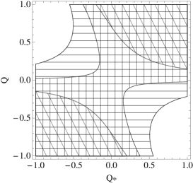
Figure 10: Regions of positive discriminant for $L=\{3.2,3.5,3.8\}$; hatching: (diagonal, vertical, horizontal); $E=0.98$

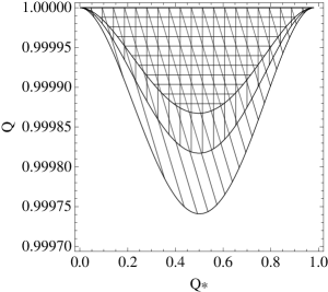
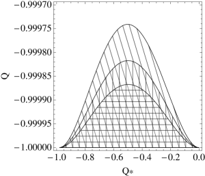
Figure 11: Regions in which the potential has three extrema that are all $>r_{+}$, for $L=\{3.2,3.5,3.8\}$; hatching: (diagonal, vertical, horizontal); $E=0.98$

This is not the complete picture. The existence of two minima outside the horizon does not imply that there are multiple stable circular orbits, because unlike in the $Q_{*}=0$ case, $\mathcal{E}_{\textrm{eff}}$ is fixed by the $E$ we chose for plotting the potential. For there to be two stable circular orbits such that an energetic particle could “roll” from one stable circular orbit over the local maximum and into the stable circular orbit, the following condition must be satisfied:

$$V_{\textrm{eff}}(r_{1},L,Q,q,E)=V_{\textrm{eff}}(r_{2},L,Q,q,E),$$ (41)

where $r_{1}$ and $r_{2}$ are the radii of stable circular orbits.

This is a special case of when the effective potential has two minima and $\mathcal{E}_{\textrm{eff}}$ cuts through the more central of them in such a way that the periastron of the orbit it defines is outside the horizon. If the general case never occurs, the special case is impossible as well. We check for the general case using a parameter plot, shown in Figure 12. Were the three regions shown in the plot ever to overlap, we would have parameters for which the potential has two minima such that $\mathcal{E}_{\textrm{eff}}$ cuts across the first minimum to yield periodic orbits. The regions in this plot do not overlap for $Q=1.0$, $L=3.6$. Regenerating the plot for various $Q$ and $L$ reveals the effect of changing each on the shape of each region and makes it clear that the three regions never overlap. We cannot expect to find any choice of parameters that yields a second region of bounded orbits in the potential’s more central minimum. This outcome does not preclude the existence of bounded orbits in the second minimum, where there are no obstacles to applying the taxonomy.

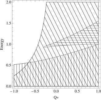
Figure 12: $Q=1.0$; $L=3.6$. Each point in the parameter plot defines an effective potential and $\mathcal{E}_{\textrm{eff}}$. The regions shown are those where the resulting orbits’ periastra are at a radius outside the horizon (horizontal hatching), where the periastra are inside the potential’s smaller minimimum (vertical hatching), and where the discriminant is positive (diagonal hatching). The coincidence of the three regions gives us the subset of parameter space in which we can find bounded orbits in the first of the potential’s two minima

IV.2 Bounds on L

The final step in characterizing the charged particle RN geometry is to calculate $L_{\textrm{ISCO}}$ and $L_{\textrm{IBCO}}$. We first write $V^{\prime}_{\textrm{eff}}$ and $V^{\prime\prime}_{\textrm{eff}}$:

$$V^{\prime}_{\textrm{eff}} = \frac{1-EQ_{*}Q}{r^{2}}+\frac{Q^{2}Q_{*}^{2}-L^{2}-Q^{2}}{r^{3}}$$

$$+\frac{3L^{2}}{r^{4}}-\frac{2L^{2}Q^{2}}{r^{5}}$$

$$V^{\prime\prime}_{\textrm{eff}} = \frac{2EQ_{*}Q-2}{r^{3}}+\frac{3L^{2}+3Q^{2}-3Q_{*}Q^{2}}{r^{4}}$$

$$-\frac{12L^{2}}{r^{5}}+\frac{10L^{2}Q^{2}}{r^{6}}$$

The condition for circular orbits is $V^{\prime}_{\textrm{eff}}=0$; solving this for $L^{2}$ and equating it with the result of solving $V_{\textrm{eff}}=0$ for $L^{2}$ yields an expression we may solve for $E_{c}^{2}$, given in Equation (44). Plugging $E_{c}^{2}$ into $L_{V^{\prime}=0}^{2}$ and simplifying yields $L_{c}^{2}$, also given below.

$$E_{c}^{2}(r,Q,Q_{*}) = \frac{\left(3Q_{*}Q^{3}-4rQQ_{*}+r^{2}QQ_{*}-B(Q^{2}-2r+r^{2})\right)^{2}}{4r^{2}(r^{2}-3r+2Q^{2})^{2}}$$

$$L_{c}^{2}(r,Q,Q_{*}) = \frac{r^{2}\left(-4Q^{4}+Q_{*}^{2}Q^{4}-6r^{2}+2r^{3}+Q^{2}r\left(10-2Q_{*}^{2}-2r+Q_{*}^{2}r\right)+B\left(Q_{*}Q^{3}+Q_{*}Qr^{2}-2Q_{*}Qr\right)\right)}{2\left(2Q^{2}-3r+r^{2}\right)^{2}}$$

$$B = \sqrt{8Q^{2}+Q^{2}Q_{*}^{2}-12r+4r^{2}}\,.$$ (44)

The ISCO exists at the inflexion point, given by $V^{\prime\prime}(r)=0$. So the solution of $L^{2}_{V^{\prime}=0}=L^{2}_{V^{\prime\prime}=0}$ for $r$ gives us $r_{\textrm{ISCO}}$. Likewise, the solution of $L^{2}_{V^{\prime}=0}=L^{2}_{V=0}$ for $r$ gives us $r_{\textrm{IBCO}}$. Plugging each of these into $L_{c}^{2}$ then yields $L_{\textrm{IBCO}}$ and $L_{\textrm{ISCO}}$. Because these solutions do not provide any additional insight, we do not reproduce them here.

Having defined the bounds in which we find periodic orbits, we can move on to applying the taxonomy to orbits in RN spacetime. The taxonomy can be used to compare the parameters that yield orbits of a given $q$ in the $Q\neq 0$, $Q_{*}=0$; $Q\neq 0$, $Q_{*}\neq 0$; and $Q=0$ cases, as we will now show.

V Periodic Tables of Orbits in RN Spacetime

V.1 Overview of the Taxonomy

Before discussing the taxonomy as it applies to the RN spacetime, we will summarize its salient features, which were presented in an earlier paper levin . As mentioned, orbits to which we can apply this taxonomy appear within the $L_{\textrm{IBCO}}$ and $L_{\textrm{ISCO}}$ of the geometry, which define the region of parameter space in which the potential accommodates bounded orbits.

The taxonomy assigns to each orbit a distinct rational number using a scheme that takes advantage of the fact that in the strong-field regime, every periodic orbit exhibits certain clearly visible topological characteristics. In this section we will discuss how to assign to each orbit a rational number based on the orbit’s topological features.

Each periodic orbit is associated with a rational number $q$, defined as

$$q=w+\frac{v}{z},$$ (45)

where $w$, $v$, and $z$ are integers. Each of these integers corresponds to a specific topological characteristic of a given periodic orbit. The most easily visualized is “z,” the number of leaves, or “zooms” in the particle’s orbit. In its path around an RN black hole, our test particle will trace out a number of leaves before closing. Figure 15 depicts orbits with various $z$ values.

The integer $w$ defines the number of “whirls” the particle makes in its path from apastron to periastron to the subsequent apastron. To understand this, note that every object travels at least a full $2\pi$ around the central black hole. The number of whirls is defined as the additional integer number of $2\pi$ executed beyond this. In other words, the number of extra turns around the center of the geometry gives us the value of $w$. Figure 15 shows orbits with various $w$ values.

We require a third number $v$, the “vertex” number, to distinguish between orbits that have equal $z$ and $w$ but are geometrically different nonetheless. This is easily seen in Figure 15, in which both orbits have $z=4$, $w=1$, but where we see that the particle can skip leaves in its motion from apastron to apastron.

Figure 13: Periodic orbits with $z$ = 1, 2, 3, and 4 for $L=3.8$, $Q=0.5$, $Q_{*}=0$

Figure 14: The $(w,v,z)=(w,0,1)$ orbits for $L=3.5$, $Q=0.5$. From left to right, these are $(0,0,1)$, $(1,0,1)$, and $(2,0,1)$. Orbits with $w>3$ are indistinguishable at this scale because the additional “whirls” are densely packed in $r$.

Figure 15: Two $z=4$, $w=1$ orbits with different $v$ values.

We label successive apastra of a periodic orbit with integers, counting the starting apastron of the orbit as $0$ and increasing in the same rotational sense as the orbit (counterclockwise for prograde orbits, clockwise for retrograde orbits), as shown in Figure 15. In general, any periodic orbit with $z>2$ can skip any number of vertices less than $z$ when moving between apastra. We define $v$ to be the index of the first vertex hit by the orbit after $v=0$ (the bounds on $v$ are therefore $1\leq v\leq z-1$). When $z=1$, we define $v=0$, which is the only sensible choice for $v$ because it implies that that successive apastra for single-leaf ($z=1$) orbits are actually the same single apastron (see Figure 15).

Finally, we must address the degeneracy that arises when the quotient $v/z$ is a reducible fraction. For a given $w$, there are multiple choices of $z$ and $v$ that describe the same orbit; for instance, when we have $q=1\frac{2}{4}$ the particle skips every other apastron and never hits vertices 1 or 3, which means it closes after only two leaves. This is equivalent to a $q=1\frac{1}{2}$ orbit. To avoid this issue, we require that $v$ and $z$ be relatively prime. The bounds on v are therefore

$$1\leq v\leq z-1 \textrm{if }z>1\;\text{and}\;z,v\;\text{are relatively prime}$$

$$v=0 \textrm{if }z=1.$$ (46)

The rational $q$ defines all of the topological features of any closed equatorial orbit and corresponds to the precession of the orbit beyond a Keplerian ellipse.

The utility of the taxonomy becomes apparent when we compare pairs of orbits with nearby $q$ values. Figure 16 depicts several pairs of orbits; each orbit in the center column may be approximated with the one in the left column.

Figure 16: A periodic table of orbits; in each column the upper orbit may be approximated by the corresponding orbit in the second row.

V.2 Comparisons Between RN and Schwarzschild

The taxonomy also gives us a way to visually inspect orbits in different spacetimes to understand whether we can distinguish between them based solely on the dynamics of their periodic orbits. For example, an important question is whether it is possible to distinguish RN orbits from Schwarzschild orbits in this way. Figures 17 and 18 depict periodic tables for the RN and Schwarzschild geomtries, respectively. By inspection, it is evident that high $w$ orbits occur at higher energies in RN spacetime than their Schwarzschild counterparts. As a result, the apastra for RN orbits with $w>0$ are consistently larger than for Schwarzschild orbits. Comparing orbits in Figure 18 to those in Figure 19 instead allows us to compare orbits with equal $q$ for the same $L$; note however that here, the RN geometry is not extremal, as $Q=0.4$. Also note that while the $q=1/2$ orbit does not exist in the $L=0.4$ Schwarzschild geometry, it can be found in the $L=3.8$, $Q=0.4$ spacetime. We still find that high $w$ orbits occur at higher energies in RN spacetime and that, again, the apastra for these orbits are consistently larger than those of their Schwarzschild counterparts.

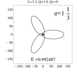
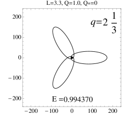
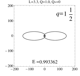
Figure 17: All extremal RN $z=$ 1, 2, 3 orbits with $w=$ 0 for the first column, $w=$ 1 for the middle column, and $w=$ 2 for the last column. For all orbits, $L=3.3$ and $Q=1.0$. Orbits increase in energy from top to bottom and left to right. Note that the first and second entries in the first column are blank because the $q=0+\frac{0}{1}$ and $q=0+\frac{1}{3}$ orbits are inaccessible.

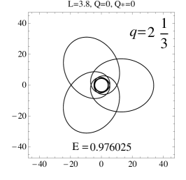
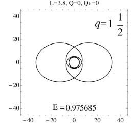
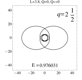
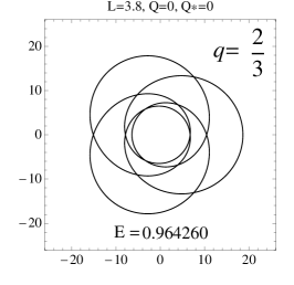
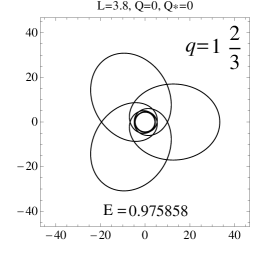
Figure 18: All Schwarzschild $z=$ 1, 2, 3 orbits with $w=$ 0 for the first column, $w=$ 1 for the middle column, and $w=$ 2 for the last column. Orbits increase in energy from top to bottom and left to right.

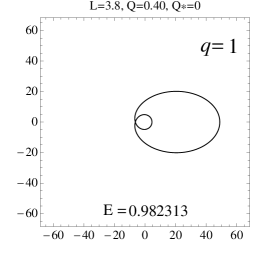
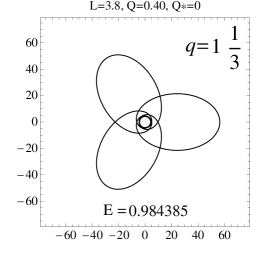
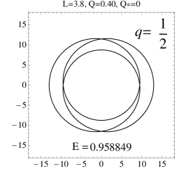
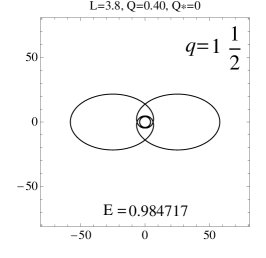
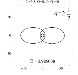
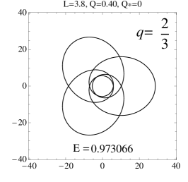
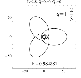
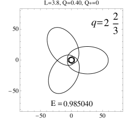
Figure 19: All RN $z=$ 1, 2, 3 orbits with $w=$ 0 for the first column, $w=$ 1 for the middle column, and $w=$ 2 for the last column. Orbits increase in energy from top to bottom and left to right.

We may use energy level diagrams, such as the one in Figure 20, to understand the relationship between $q$ and $E$ in each spacetime (for a general discussion, see levin_el ). These diagrams make it clear that RN orbits do appear at a higher set of energies. Next we want to look at how the spacing between these energies varies. Figure 21 shows the differences between values of $E$ for successive orbits in the RN and Schwarzschild cases.

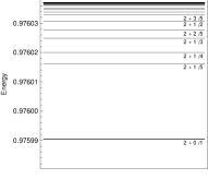
Figure 20: Energy levels for Schwarzschild orbits (first row) with $L=3.8$ and RN Orbits (second row) with $L=3.3$, $Q=1.0$, $Q_{*}=0$. The second and fourth figures show detail of the first and third figures, respectively, indicating the rationals within the $w=3$ band. These diagrams show lines for all orbits with $w\in(2,3,4,5,6)$, $z\in(1,2,3,4,5)$ with $v<z$ and $v$ and $z$ coprime.

We find that not only are the RN energies collectively higher, they spacing between each pair of energies is also consistently larger than in the Schwarzschild case. Furthermore, the magnitude of difference between spacings in each geometry increases. The ratio of the energy difference in the RN and Schwarzschild $q=2$ and $q=2\frac{1}{5}$ orbits is $3.52$, but this rises to $23.41$ when we compare the difference between the $q=6$ and $q=6\frac{1}{5}$ orbits in each geometry.

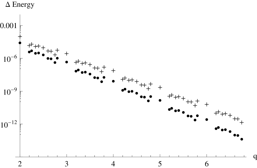
Figure 21: Differences in energies at which we find orbits of various $q$ in the RN (marked with “$+$”) and Schwarzschild (marked with “$\cdot$”) spacetimes.

VI Conclusions

We have applied the taxonomy of levin to the Reissner-Nordström spacetime and demonstrated that within certain bounds for $Q$ and $L$, the orbital dynamics can be characterized using zoom-whirl behavior. These bounds were calculated for both the charged and uncharged particle cases. Furthermore it was demonstrated that the regions in which we find bounded orbits in RN spacetime are analogous to those in Schwarzschild spacetime, and that we do not find multiple stable circular orbits for any choice of parameters within our predefined bounds. Applying the taxonomy to RN spacetime for both charged and uncharged particles enables us to differentiate between the set of periodic orbits in each geometry based on their orbital dynamics. We find not only that RN orbits occur at higher energies than their Schwarzschild counterparts, but that this is a behavior that persists for various $Q$. Furthermore, we find that RN orbits of a given $q$ are more eccentric than their Schwarzschild equivalents.

VII Acknowledgments

We are especially grateful to Alberto Nicolis for valuable discussions of this work. J. L. and V. M. acknowledge financial support from NSF grant AST-0908365. This material is based in part upon work supported by a scholarship from the Rabi Scholars program at Columbia University.

Appendix A Hamiltonian formulation of RN geodesic motion

For completeness we present a Hamiltonian formulation of RN motion. These were the equations integrated to generate the orbits in the paper. We begin with the Lagrangian density for a free particle in Reissner-Nordström spacetime:

$$\mathcal{L}=\frac{1}{2}g_{\alpha\beta}\dot{q}^{\alpha}\dot{q}^{\beta}.$$ (47)

The $q^{\alpha}$ are dimensionless coordinates, as we have assumed that the orbiting particle is of unit mass. Furthermore, for timelike trajectories, $\mathcal{L}=-1/2$. Using

$$p_{\alpha}\equiv\frac{\partial\mathcal{L}}{\partial\dot{q}^{\alpha}}$$ (48)

we obtain the components of the momentum:

$$p_{t} = \frac{\partial\mathcal{L}}{\partial\dot{t}}=-\Delta\,\dot{t}$$ (49)

$$p_{r} = \frac{\partial\mathcal{L}}{\partial\dot{r}}=\Delta^{-1}\,\dot{r}$$ (50)

$$p_{\theta} = \frac{\partial\mathcal{L}}{\partial\dot{\theta}}=r^{2}\dot{\theta}$$ (51)

$$p_{\phi} = \frac{\partial\mathcal{L}}{\partial\dot{\phi}}=r^{2}\sin^{2}\theta\,\dot{\phi}.$$ (52)

The Hamiltonian is then defined

$$\mathcal{H}=p_{\mu}\dot{q}^{\mu}-\mathcal{L}$$ (53)

Like the $q^{\alpha}$, the particle’s 4-momentum is also dimensionless and is here equivalent to the 4-velocity (since $\mu$, the particle mass, is set equal to 1). So we may write Equation (53) as

$$\mathcal{H}=\frac{1}{2}g^{\alpha\beta}p_{\alpha}p_{\beta}.$$ (54)

If we compute $\mathcal{H}$ we find that

$$\mathcal{H} = \frac{1}{2}\Big{(}-\Delta^{-1}(-\Delta\dot{t})^{2}+\Delta^{-1}(\Delta\dot{r})^{2}+$$

$$r^{-2}(r^{2}\dot{\theta})^{2}+r^{-2}\sin^{-2}\theta(r^{2}\sin^{2}\theta\dot{\phi})^{2}\Big{)}$$

$$= \frac{1}{2}\left(-\Delta\dot{t}^{2}+\Delta^{-1}\dot{r}^{2}+r^{2}\dot{\theta}^{2}+r^{2}\sin^{2}\theta\dot{\phi}^{2}\right)$$

$$= \mathcal{L}.$$

Because each quantity in the Hamiltonian is just half the contraction of the 4-momentum, it is identical to the Lagrangian, which is not surprising because our Lagrangian and Hamiltonian contain only kinetic terms levin .

Next we wish to plug our Hamiltonian into Hamilton’s equations,

$$\dot{q}_{i}=\frac{\partial\mathcal{H}}{\partial p_{i}}\hskip 36.135pt\dot{p}_{i}=\frac{\partial\mathcal{H}}{\partial q_{i}},$$ (56)

which requires that we rewrite $\mathcal{H}$ in terms of the $p_{i}$. Hamilton’s equations give us explicitly

$$\frac{\partial\mathcal{H}}{\partial p_{r}}=\dot{r} = \Delta\cdot p_{r}$$ (57)

$$\frac{\partial\mathcal{H}}{\partial p_{t}}=\dot{t} = -\Delta^{-1}\cdot p_{t}$$

$$\frac{\partial\mathcal{H}}{\partial p_{r}}=\dot{\theta} = r^{-2}\cdot p_{\theta}$$

$$\frac{\partial\mathcal{H}}{\partial p_{r}}=\dot{\phi} = r^{-2}\sin^{-2}\theta\cdot p_{\theta}$$

for the $\dot{q}_{i}$ and, for the $\dot{p}_{i}$,

$$\dot{p}_{t}=-\frac{\partial\mathcal{H}}{\partial t} = 0$$ (58)

$$\dot{p}_{r}=-\frac{\partial\mathcal{H}}{\partial r} = -\dot{\theta}^{2}r-\sin^{2}\theta\dot{\phi}^{2}r+$$

$$\left(\frac{1}{r^{2}}-\frac{Q^{2}}{r^{3}}\right)\left(\frac{\dot{r}^{2}}{\Delta^{2}}+\dot{t}^{2}\right)$$

$$\dot{p}_{\theta}=-\frac{\partial\mathcal{H}}{\partial\theta} = -r^{2}\dot{\phi}^{2}\sin\theta\cos\theta$$

$$\dot{p}_{\phi}=-\frac{\partial\mathcal{H}}{\partial\phi} = 0.$$

The equations above were used in the numerical results presented in the body of the paper.

References

- (1) E. Flanagan and S. Hughes, Phys. Rev. D 57 (1998).
- (2) K. Glampedakis, S. Hughes, and D. Kennefick, Phys. Rev. D 66 (2002).
- (3) S. Drasco and S. Hughes, Phys. Rev. D 69 (2005).
- (4) E. Drasco and S. Hughes, Class. Quant. Grav 22 (2005).
- (5) S. Drasco and S. Hughes, Phys. Rev. D (2006).
- (6) R. N. Lang and S. A. Hughes, Phys. Rev. D 74 (2006).
- (7) K. Glampedakis and D. Kennefick, Phys. Rev. D. 66.
- (8) L. Grishchuk et al., Physics–Uspekhi 44 (1), 1 (2001).
- (9) J. Levin and G. Perez-Giz, Phys. Rev. D 79 (2009).
- (10) J. Levin, Class. Quantum Grav. 29.
- (11) J. Levin and B. Grossman, Phys. Rev. D 79.
- (12) R. Grossman and J. Levin, Phys. Rev. D. 79.
- (13) S. Carroll, Spacetime and Geometry: An Introduction to Special Relativity, Addison-Wesley, 2003.
- (14) L. Barack and C. Cutler, Phys. Rev. D 69 (2004).
- (15) S. Chandrasekhar, The Mathematical Theory of Black Holes, Oxford: Clarendon Press, 1998.
- (16) J. Levin and G. Perez-Giz, Phys. Rev. D 77.
- (17) J. Levin and G. Perez-Giz, Phys. Rev. D 79.