Maximally entangled states in the Hydrogen molecule: The role of spin and correlation

Abstract

By going beyond Hubbard Hamiltonian we reflected correlation effects accurately in the wavefunctions of $H_{2}$. Using $ab$ $initio$ e-e interaction parameters resulted maximally entangled ground and third excited states. We assigned this maximally entangled character to the nonmagnetic (S=0) property of these states and also the minimally entangled character of the first excited states to its magnetic property (S$\neq 0$). By switching on a magnetic field an entangled state with $S_{z}=0$ can be extracted from a minimally entangled degenerate magnetic state. We suggest that presence of a moderate correlated system and a non-magnetic $(S_{z}=0)$ electronic state can be two criteria for finding maximally entangled electronic states in a realistic molecular system.

1 Introduction

Since Einstein, Podolsky and Rosen [1] and Schrödinger [2] investigated the non-classical properties of quantum systems and entered new concept as entanglement in quantum physics, it had become strange property in interaction between particles. Recently the study of the entanglement is a useful resource for quantum communications and information processing [3] such as quantum teleportation [4, 5], superdense coding [6], quantum key distribution [7], and quantum cryptography [8] whose input states are constructed to be maximally entangled. Also entanglement has been suggested as a quantitative measure for electron-electron (e-e) correlation in many body systems [9, 10]. As a simple illustration of entanglement we can say that, if there is no way to write the states of two particles as a product of the two systems states in the Hilbert space, then there will be an entangled system [11]. A lot of investigation has been done about measuring entanglement in the fermionic systems, such as the Wooters’ measure [12] and the Schliemann’s measure [13, 14]. Through Gittings’ investigation [15], it is shown that all these entanglement measures are not suitable but the Zanardi’s measure [16, 17] satisfies all desirable properties of entanglement measurement.
The $H_{2}$ molecule is the simplest two electron systems that can be used to implement a robust many body calculation based on Hubbard model [18]. Traditional Hubbard model which is a priory many-body approach usually is used as a first attempt to calculate entanglement. This model gives maximum entanglement by setting e-e interaction parameter $U=0$, which is a controversial conclusion [17, 19, 20]. In this paper we go beyond Hubbard model to calculate entanglement of the non-magnetic ground and magnetic excited states of $H_{2}$ molecule. The $H_{2}$ molecule is the simplest realistic two electron correlated system in nature which our model can be implemented and considering all direct and exchange interaction terms beyond Hubbard model let us account correlation effects more accurately in the wavefunctions. The Zanardi measurement for calculating entanglement was employed. We will investigate the ground and excited state of $H_{2}$ to find the effect of the spin on the entanglement of states and results give maximally entangled states with non-zero U value. We also discuss the difference between maximally, moderately and zero entangled states based on their magnetic property and correlation dependence.

2 Calculation method

Now we explain our calculation method. The complete Hubbard Hamiltonian is defined as [21]:

$$H=\sum_{ij\sigma}t_{ij}c^{\dagger}_{i\sigma}c_{j\sigma}+\frac{1}{2}\sum_{ijlm\sigma\sigma^{\prime}}V_{ijlm}c^{\dagger}_{i\sigma}c^{\dagger}_{j\sigma^{\prime}}c_{m\sigma^{\prime}}c_{l\sigma}.$$ (1)

The first term contains non-interacting part of Hamiltonian which can be written as:

$$\sum_{ij\sigma}t_{ij}c^{\dagger}_{i\sigma}c_{j\sigma}=\varepsilon_{\circ}\sum_{i=1,2;\sigma}c^{\dagger}_{i\sigma}c_{i\sigma}+t\sum_{i\neq j;\sigma}c^{\dagger}_{i\sigma}c_{j\sigma}$$ (2)

$$t_{21}=t_{12}=t$$

where $\varepsilon_{\circ}$ is the energy of atomic orbital, $c^{\dagger}_{i\sigma}$ and $c_{i\sigma}$ are fermionic creation and annihilation operators on site i with spin $\sigma$, respectively and t stands for the hopping integral between two H atomic sites of the electrons with the same $\sigma$. The second term of Hamiltonian that contains e-e interaction part can also be written as:

$$\frac{1}{2}\sum_{ijlm\sigma\sigma^{\prime}}V_{ijlm}c^{\dagger}_{i\sigma}c^{\dagger}_{j\sigma^{\prime}}c_{m\sigma^{\prime}}c_{l\sigma} = U\sum_{i=1,2}n_{i\uparrow}n_{i\downarrow}+\frac{1}{2}J\sum_{i\neq j;\sigma\sigma^{\prime}}n_{i\sigma}n_{j\sigma^{\prime}}$$ (3)

$$+\frac{1}{2}X_{1}\sum_{ijlm\sigma\sigma^{\prime}}c^{\dagger}_{i\sigma}c^{\dagger}_{j\sigma^{\prime}}c_{m\sigma^{\prime}}c_{l\sigma} + \frac{1}{2}X_{2}\sum_{ijlm\sigma\sigma^{\prime}}c^{\dagger}_{i\sigma}c^{\dagger}_{j\sigma^{\prime}}c_{m\sigma^{\prime}}c_{l\sigma}$$ (4)

where $V_{ijlm}$ contains all coulomb interaction between electrons which involves U as on-site Coulomb repulsion, J as inter-site Coulomb repulsion and $n_{i\sigma}=c^{\dagger}_{i\sigma}c_{i\sigma}$ is density operator. The last terms $X_{1}$ and $X_{2}$ are the exchange interactions parameters that can be interpreted by quantum mechanics. We consider two electrons in two sites or $1s$ orbital of $H_{2}$ molecule with spin up and down, therefore we have four states for a single electron so for two electrons there are $C(4,2)=6$ states which are represented with notation $|\varphi>=|n_{1\uparrow}n_{1\downarrow}n_{2\uparrow}n_{2\downarrow}>$ as

$$|\varphi_{1}> = |1100>,|\varphi_{2}>=|1010>,|\varphi_{3}>=|1001>$$ (5)

$$|\varphi_{4}> = |0110>,|\varphi_{5}>=|0101>,|\varphi_{6}>=|0011>$$ (6)

With these sets of states, we can write Hamiltonian as:

$$H=\left(\begin{array}[]{cccccc}U&0&t+X_{1}&-t-X_{1}&0&X_{2}\\ 0&J-X_{2}&0&0&0&0\\ t+X_{1}&0&J&-X_{2}&0&t+X_{1}\\ -t-X_{1}&0&-X_{2}&J&0&-t-X_{1}\\ 0&0&0&0&J-X_{2}&0\\ X_{2}&0&t+X_{1}&-t-X_{1}&0&U\\ \end{array}\right).$$

All the diagonal elements contain a term $t_{ii}$, where it is roughly four times of the energy of an electron in the $1s$ state of atomic hydrogen. Using $ab$ $initio$ energies for $H_{2}$ and $H_{2}^{+}$ from Ref. [22] and with the parametric energies of Hamiltonian, parameters $\varepsilon_{\circ}$, t, U, J, $X_{1}$ and $X_{2}$, were evaluated and are given in Table I.

Table 1: The calculated values of Hamiltonian parameters.

Hamiltonian parameter	$\varepsilon_{\circ}$	$t$	$U$	$J$	$X_{1}$	$X_{2}$
calculated value(eV)	-28.56	6.36	19.68	17.90	0.95	1.36

Entanglement measurement is defined by von Neumann’s entropy as[16]:

$$S(\rho_{A})=-tr(\rho_{A}\log_{2}\rho_{A})$$ (7)

where $A$ and $B$ are bipartite subsystem which in our model are $1s$ orbital of each Hydrogen atoms in our model. $\rho_{A}$ is reduced density matrix that is defined by:

$$\rho_{A}=tr_{B}\rho_{0}=\sum_{j}<j|_{B}(|\psi><\psi|)|j>_{B}$$

where $tr_{B}$ stands for tracing over all sites except the $B$ sites and $\mid j>_{B}$ is eigenstate for $B$ part $(|n_{2\uparrow}n_{2\downarrow}>)$ i.e. $\mid 00>,\mid 01>,\mid 10>and\mid 11>$. After these calculation the reduced density matrix for the ground state (not normalized) becomes:

$$\rho_{A}=tr_{A}|\psi\rangle\langle\psi|=\left(\begin{array}[]{cccc}1&0&0&0\\ 0&\alpha_{+}^{2}&0&0\\ 0&0&\alpha_{+}^{2}&0\\ 0&0&0&1\\ \end{array}\right).$$ (8)

For other states, reduced density matrices have been evaluated accordingly and their entanglements were calculated. We listed the resultant entanglement values in Table II.

Table 2: The parametric energies of hydrogen molecule are listed in the first column of the Table, where $\alpha_{\pm}(x)=x\pm\sqrt{1+x^{2}}$ and $x=\frac{(U-J)}{4(t+X_{1})}$. The values of energies from Ref. [22] are listed in the second column, eigenfunction for these states are also listed in the third column. The $S^{2}$ and $S_{z}$ of each state are given in the next columns and the last column is the calculated entanglement $S(\rho_{A})$ for these states, based on Zanardi’s measurement.

E	E(eV)	$\psi$	$S^{2}$	$S_{z}$	$S(\rho_{A})$
$E_{0}=2\varepsilon_{\circ}+X_{2}+J+2(t+X_{1})\alpha_{-}(x)$	-51.60	$\varphi_{1}+\varphi_{6}+\alpha_{+}(x)(\varphi_{4}-\varphi_{3})$	0	0	$\sim 2$
$E_{1}=2\varepsilon_{\circ}+J-X_{2}$	-40.58	$\varphi_{3}+\varphi_{4}$	2	0	1
$E_{1}=2\varepsilon_{\circ}+J-X_{2}$	-40.58	$\varphi_{2}$	2	1	0
$E_{1}=2\varepsilon_{\circ}+J-X_{2}$	-40.58	$\varphi_{5}$	2	-1	0
$E_{2}=2\varepsilon_{\circ}+U-X_{2}$	-38.80	$\varphi_{6}-\varphi_{1}$	0	0	1
$E_{3}=2\varepsilon_{\circ}+X_{2}+J+2(t+X_{1})\alpha_{+}(x)$	-22.32	$\varphi_{1}+\varphi_{6}+\alpha_{-}(x)(\varphi_{4}-\varphi_{3})$	0	0	$\sim 2$

By acting $S^{2}$ on the $|E_{0}\rangle,...,\;{\rm and}\;|E_{3}\rangle$ eigenstates, we could find total spin of each state in which $|E_{0}\rangle,\;|E_{2}\rangle\;{\rm and}\;|E_{3}\rangle$ have $S^{2}=0$, but $|E_{1}\rangle$ has $S^{2}=2$. We find eigenvalues and eigenstates (not normalized) of hydrogen molecule as shown in Table II, where $\alpha_{\pm}(x)=x\pm\sqrt{1+x^{2}}$ and $x=\frac{(U-J)}{4(t+X_{1})}$. Also the related $S_{z}$ values of each eigenstates have been summarized in Table II. The eigenstates results schematically demonstrated in Fig. 1. Now let us discuss calculation results summarized in Table II and Fig.1.

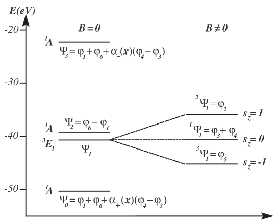
Figure 1: The ground and excited states for $H_{2}$ molecule before and after switching on a magnetic field with their related eigenfunctions and spins.

3 Results and discussion

From this table we conclude that the many electron wavefunctions have very weaker dependence on the interaction parameters than the energy levels. The wavefunctions of the first and second excited states are explicitly independent from Hamiltonian parameters. The wavefunction of the ground and third excited state are dependent upon $e-e$ correlation parameters via $\alpha_{\pm}=x\pm\sqrt{1+x^{2}}$ with $x=\frac{(U-J)}{4(t+X_{1})}$ in Table II where the exchange interaction $X_{2}$ is absent in the wavefunctions. Both of these states are nonmagnetic (S=0). Using parameters of Table I and von Neumann’s entropy of Eq. (6) an entanglement value $S[\rho]\sim 2$ was obtained for these states. The maximum available value of entanglement is $log_{2}d$ for a system with the Hilbert space dimension of the smaller subsystem as $d$ [23]. Accordingly, for $H_{2}$ molecule the maximum available entanglement is 2 therefore the resultant maximally entangled ground and third excited states in Table II can be explained by the corresponding wave functions of these states. The wavefunctions of the ground and third excited states are superposition of four body basis of the systems $\varphi_{1},\;\;\varphi_{3},\;\;\varphi_{4}\;\;{\rm and}\;\;\varphi_{6}$ with equal coefficients since the value of $\alpha_{\pm}$ from table I becomes 1.
From Table II, the first excited state $E_{1}$ is a spin triplet state with $S=1$ and its wavefunction is independent fromcorrelation parameters. The value of entanglement for the $S_{z}=0$ eignfunction is 1 where its value for the eignfunctions with $S_{z}=\pm 1$ is zero. The difference between entanglements of the degenerate wavefunctions with different $S_{z}$ can be explained by their related wavefunctions. The entanglement of the eignfunction of $|E_{1},S_{z}=0\rangle$ state is a linear combination of $\varphi_{3}$ and $\varphi_{4}$ whereas the wave functions of other $|E_{1},S_{z}=\pm 1\rangle$ are separable ($\varphi_{2}$ or $\varphi_{5}$). The importance of the nonzero spin of the first excited state is that this state can be detected by Electron paramagnetic resonance (EPR) under some condition [24]. When the magnetic field is off the wavefunction is a superposition of the degenerate wavefunctions with different $S_{z}$ values. We calculated entanglement of this degenerate wavefunction as 0. However, after switching on the magnetic field, a wavefunction with definite value of entanglement emerges. The values of the $S_{z}$ and entanglement for this state are 0 and 1 according to Table II. Therefore we conclude that in practice by switching on a magnetic field on a magnetic state, one can switch from a degenerate and not entangled wavefunction to an entangled wavefunction with $S_{z}=0$.
The second excited state $E_{2}$ is nonmagnetic, $S=0$, where the wavefunction is independent from correlation parameters. The calculated entanglement is 1. The wavefunction of this state is only a linear combination of two basis set $\varphi_{6}$ and $\varphi_{1}$, hence its entanglement is smaller than ground and third excited states. By comparing the values of the entanglement listed in Table II, we conclude that the nonmagnetic states $(S=0)$ in which the wavefunction depend on interaction parameters are maximally entangled and the magnetic states whose wavefunctions are independent from correlation parameters are not entangled.
Using von neumann’s entropy in Eq. 6, we calculated the variation of entanglement for maximally entangled ground state of $H_{2}$ molecule with respect to the combination of correlation parameters $x=\frac{(U-J)}{4(t+X_{1})}$. Results were plotted in Fig. 2.

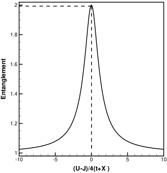
Figure 2: Entanglement for the ground state of Hydrogen molecule versus $e-e$ interaction parameters.

In this figure we observe that the value of entanglement is maximum with $x=0$ ($U=J$). This conclusion resolves previously reported results from other groups [17, 19, 20] who obtained maximally entangled ground state with $U=0$. The $U=0$ result imply that the maximally entangled ground state is not attainable for the $H_{2}$ since the $ab$ $initio$ value of $U$ from Table I is $19.68$ which is very far from zero. In our given model the maximally entangled ground state obtained with U=J. This has a meaningful physical interpretation which states that in such physical system where the inter-atomic distance is very small, the on-site Columbic repulsion U can be very close to the inter-site Columbic repulsion J. Indeed the $H_{2}$ molecule is the best example of such systems when the inter-atomic distance is minimum or $d=0.7{\AA}$ and the $ab$ $initio$ value of U and V from Table II gives $x=0.06$. Using $ab$ $initio$ parameters of Table I, we obtained $x=0.06$ and this value of x gives maximally entangled ground state. From Fig.2 the maximum entanglement value for $x=0.06$ is 1.99.
As we observe in Fig. 2, in the extreme limit of $|\frac{U}{t}|\gg 1$, i.e. strongly correlated systems the entanglement becomes smaller and tends to 1. The non-magnetic property of this state, sets a limit on minimum available entanglement for this state. This point can be explained by using eigenfunction listed in Table II. For $|x|\gg 1$ one of the $\alpha_{+}$ or $\alpha_{-}$ goes to zero and the other one becomes very large. In both cases the ground state wavefunctions listed in Table II reduce from extension on the four components to an extension on the two components similar to $|E_{2}\rangle$ state. Therefore the corresponding value of entanglement reduces from 2 to 1. This also can be explained by tendency of the strongly correlated systems with $|\frac{U}{t}|\gg 1$ to unpaired electronic configuration in atomic orbital such as $\varphi_{2}$ and $\varphi_{5}$ states in which energy reduces by loosing U term in Hamiltonian. Such states tend to have parallel spin and magnetism with a reduced entanglement.
In the case of $H_{2}$ where $t$, $U$ and $J$ are at the same order of magnitude (See Table I) and $x$ is much close to zero hence the molecule is in moderately correlated regime and one can obtain the maximum available entanglement as it is shown in Fig. 2. In this regime we have both spatial and spin correlated wave function[17]. Neglecting exchange interaction in our model ($X_{1}=X_{2}=0$), significantly displaces energy levels of the system (see Table II). However, the dependence of the ground and third excited state wavefunctions on the exchange parameters only is limited to $X_{1}$ and putting $X_{1}=0$ yields $x=0.07$ and similarly the maximum entanglement becomes 1.99 which is the same as the case of nonzero $X_{1}$ ($x=0.06$). In otherwords in order to obtain maximally entangled states, the most effective parameters are direct columbic interaction parameters $U$ and $J$ and exchange interaction parameters do not alter the value of entanglement significantly.

4 conclusion

In conclusion, in this paper we applied a robust many electron calculation on a simplest realistic two electron system i. e. $H_{2}$ molecule. Going beyond traditional Hubbard model let us to account correlation effects accurately in the many electron wavefunction of the ground and excited states. Using $ab$ $initio$ e-e interaction parameters, indicates to a moderately correlated regime for the molecule and resulted a maximally entangled ground and third excited state. The wavefunctions of the not magnetic (S=0) ground and excited states explicitly depend on correlation parameters whereas the first excited states which is magnetic ($S^{2}=2$ and $S_{z}\neq 0$) is not entangled. The second excited state is not magnetic but its wavefunction does not depend on correlation parameters therefore it is a moderately entangled state. Anycase, by switching on a magnetic field an entangled state with $S_{z}=0$ can be extracted from a not entangled degenerate magnetic state. We suggest that in a realistic molecular scale systems, there is two criteria for finding maximally entangled electronic states, first the system should be in moderately correlated regime and second the system should have a non-magnetic $(S_{z}=0)$ electronic state.

References

- [1] A. Einstein, B. Podolsky, and N. Rosen, Phys. Rev. 47, 777 (1935).
- [2] E. Schrdinger, Proc. Cambridge Phill. Soc. 31 555 (1935).
- [3] C. Macchiavello, G.M. Palma and A. Zeilinger, Quantum Computation and Quantum Information Theory (World Scientific, Singapour, 2000).
- [4] C.H. Bennett ,G. Brassard, C. Crépeau, R. Jozsa, A. Peres and W. K. Wootters, Phys. Rev. Lett. 70, 1895 (1993).
- [5] D. Bouwmeester et al. Nature, 390, 575(1997).
- [6] C.H. Bennett and S.J.Wiesner, Phys. Rev. Lett. 69, 2881 (1992).
- [7] A.K. Ekert, Phys. Rev. Lett. 67, 661 (1991).
- [8] C. A. Fuchs,Phys. Rev. Lett. 79, 1162 (1997).
- [9] Z. Huang, S. Kias, Chem. Phys. Lett. 413 (2005).
- [10] T.A.C.Maiolo, F.della Sala, L.Martina, and G. Soliani, Theo. and Math. Phys. 152(2) (2007).
- [11] Y.S. Li, B. Zeng, X.S. Liu, G.L. Long, quant-ph/0104101v1.
- [12] W. K. Wootters, Phys. Rev. Lett. 80, 2245 (1998).
- [13] J. Schliemann, D. Loss, and A.H. MacDonald, e-print cond-mat/0009083.
- [14] J. Schliemann, J. Ignacio Cirac, M. Kus, M. Lewenstein and D. Loss, Phys. Rev. A 64, 022303 (2001).
- [15] J. R. Gittings and A. J. Fisher, phys. Rev. A 66 032305 (2002).
- [16] P. Zanardi, Phys. Rev. A 67, 054301 (2003).
- [17] P. Zanardi, Phys. Rev. A 65 042101 (2002).
- [18] B Alvarez-Fernndez and J A Blanco Eur. J. Phys. 23 11 (2002)
- [19] H. Wang, S. kias, Chem. Phys. Lett. 421, 338 (2006).
- [20] S.-J. Gu, S.-S. Deng, Y.-Q. Li, and H.-Q. Lin, Phys. Rev. Lett. 93 086402 (2004).
- [21] M. Heidari Saani, M. A. Vesaghi, K. Esfarjani, T. Ghods Elahi, M. Sayari, H. Hashemi, and N. Gorjizadeh al. Phys. Rev. B 71, 035202 (2005).
- [22] G. Chiappe, E. Louis, E. SanFabián, and J.A. Verges, phys. Rev B 75 195104 (2007).
- [23] C. H. Bennett, H. J. Bernstein, S. Popescu and B.Schumacher, phys. Rev. A 53 (1996)
- [24] J. A. Vanwyk, O. D. Tucker, M.E. Newton, J. M. Baker, G. S. Woods and P. Spear, Phys. Rev. B 52, 12657 (1995).