Bounding the Equilibrium Distribution of
Markov Population Models

I Introduction

Markov population models (MPMs) are continuous-time Markov chains (CTMCs) that describe the dynamics and interactions of different populations. They have important applications in the life science domain, in particular in ecology, epidemics, and biochemistry. Depending on the system under study, a member of a population represents an individual that belongs to a certain biological species, an organism that suffers from an infectious disease, or a certain type of molecule in a living cell. Thus, if $n$ is the number of populations, the state space of the MPM is $\mathbb{N}^{n}$, that is, a state is a vector $(x_{1},\ldots,x_{n})$ of non-negative integers, where the entry $x_{i}$ is the size of the $i$-th population. Typically, the transitions of an MPM are described by a finite set of transition classes such that each class specifies a (possibly infinite) number of edges in the underlying transition graph. For instance, we may have one class to represent the death of individuals. In biochemistry, each chemical reaction describes a class of transitions in the associated MPM. Often, the corresponding transition rates are state-dependent, e.g., the rate at which individuals of a certain population die may depend on the population size.

The structural regularity of MPMs often enables accurate approximations of the system behavior. One such example is the widely-used deterministic approximation of the dynamics of chemical reaction networks [7] that represents the states as a continuum. But if one or more populations are small a discrete representation of the population sizes is important and continuous approximations are inaccurate. This effect has also been observed experimentally in the context of chemical reactions [13, 12, 10]. In such cases the analysis of the MPM becomes difficult. Closed-form solutions are only possible in special circumstances [6] and numerical solution techniques suffer from the problem that a very large or even infinite state space has to be explored. Therefore, Monte-Carlo simulation is in widespread use to estimate transient or stationary measures of the MPM.

Recently, progress has been made on numerically approximating the transient distribution of an MPM at particular time instances [3, 5, 11]. These approaches exploit the fact that only a subset of the state space is needed to give an accurate approximation and that only a small amount of probability mass is located above a certain population threshold. The intuitive explanation for this is simple since within a fixed time interval it is extremely unlikely that the populations reach certain thresholds. For the long-run behavior of the system, however, this argument does not hold since it is a priori not known if and where the system stabilizes.

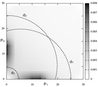
Figure 1: The equilibrium distribution $\pi$ of an MPM that describes a gene regulatory network and geometric bounds enclosing a subset $\mathcal{C}$ of the state space with $\sum_{c\in\mathcal{C}}\pi(c)>0.9$.

In this paper, we consider the problem of computing an accurate approximation of the equilibrium distribution of an MPM. Assuming that the MPM is ergodic, we first derive geometric bounds for the equilibrium distribution, i.e., we find those regions of the state space, where most of the probability mass is located in the limit. Then we perform a local refinement for these regions in order to bound the probabilities of individual states.

Let $\{X(t),t\geq 0\}$ be an MPM. The first step relies on an analysis of a drift function $d$ that associates with each state $x$ the expected change $d(x)=\frac{d}{dt}E[g(X(t))\mid X(t)=x]$. Here, $g$ is a function that associates with each state $x$ a non-negative real number, also called Lyapunov function. We illustrate this by means of an example. Figure 1 shows the plot of the equilibrium distribution of an MPM that describes a gene regulatory network. The system is bistable, that is, in the long-run the probability mass is concentrated at two distinct regions in the state space. In these regions the drift $d(x)$ is maximal. We determine geometric bounds (here depicted as dashed lines) by using a simple threshold on the drift, i.e., we consider the set $\mathcal{C}$ of all states where the drift is greater than a certain threshold. Then $\mathcal{C}$ contains those states, where most of the probability mass is located in equilibrium. For the amount of probability within $\mathcal{C}$, we derive tight bounds.

In the second step of our approach, we consider the stochastic complement of $\mathcal{C}$ [9] which allows us to derive bounds for the probabilities of individual states. The stochastic complement is a finite CTMC with state space $\mathcal{C}$, where each outgoing transition leading to a state not in $\mathcal{C}$ is redirected to $\mathcal{C}$. This redirection is defined in such a way that the equilibrium distribution of the stochastic complement gives the conditional equilibrium probabilities for the states of $\mathcal{C}$. Since the exact redirection probability can only be obtained from a full solution of the infinite system, we consider candidates that give upper and lower bounds. Together with the first step of the approach, this yields bounds for the equilibrium probabilities of all states of the MPM $X$.

The full paper version will contain all relevant proof details.

II Markov Population Models

We consider a class of time-homogeneous CTMCs that can be described by a finite set of transition classes. A transition class $\tau$ is a pair $(\alpha,v)$, where $\alpha:\mathbb{N}^{n}\to\mathbb{R}_{\geq 0}$ is a function that determines the transition rate and $v\in\mathbb{Z}^{n}$ is a change vector that determines the successor state of the transition. Thus, if $x\in\mathbb{N}^{n}$ and $\alpha(x)>0$ then there is a transition from state $x$ to state $x+v$ with rate $\alpha(x)$. We assume that $v$ has at least one nonzero entry and that $\alpha(x)$ is a polynomial in $x=(x_{1},\ldots,x_{n})$. Let $\{\tau_{1},\ldots,\tau_{k}\}$ be a set of transition classes with distinct change vectors. Let $\mathbf{Q}$ be the infinite matrix such that the entry $\mathbf{Q}(x,x+v_{j})$ equals $\alpha_{j}(x)$, where $\tau_{j}=(\alpha_{j},v_{j})$ and $j\in\{1,\ldots,k\}$. If we define the diagonal entries of $\mathbf{Q}$ as the negative sum of the off-diagonal entries, then $\mathbf{Q}$ is the infinitesimal generator of a CTMC $\{X(t),t\geq 0\}$. The matrix $\mathbf{Q}$ has only finitely many nonzero entries in each row and in each column, i.e., $\mathbf{Q}$ is an infinite matrix with finite rows/columns. Note that $\sup_{x}|\mathbf{Q}(x,x)|$ may be infinite and that the number of states reachable from a given initial state may be infinite.

III Geometric Bounds

We assume that $\tau_{1},\ldots,\tau_{k}$ are such that $X$ is ergodic and $\pi$ is the equilibrium distribution of $X$. Then there exists a function $g^{*}:\mathbb{N}^{n}\to\mathbb{R}_{+}$, a finite subset $\mathcal{C}$, and a constant $\gamma>0$ such that [14]

$$\begin{array}[]{l@{\,}c@{\ }l}(i)&\frac{d}{dt}E[g^{*}(X(t))\mid X(t)=x]\leq-\gamma,&\forall x\in\mathbb{N}^{n}\setminus\mathcal{C},\\[4.30554pt] (ii)&\frac{d}{dt}E[g^{*}(X(t))\mid X(t)=x]<\infty,&\forall x\in\mathcal{C},\\[4.30554pt] (iii)&\lx@intercol\{x\in\mathbb{N}^{n}\mid g^{*}(x)\leq\ell\}\mbox{ is finite for any }\ell<\infty.\hfil\lx@intercol\end{array}$$ (1)

Let $c$ be a positive number with $c\geq\max_{x\in\mathcal{C}}E[g^{*}(X(t))\mid X(t)=x]$ and let $g(x)=\frac{g^{*}(x)}{\gamma+c}$. In the sequel, we will refer to $g$ as the Lyapunov function. The first two conditions in Eq. (1) are now equivalent to

$$\begin{array}[]{lcl}\frac{d}{dt}E[g(X(t))\mid X(t)=x]&\leq&\frac{c}{c+\gamma}-\bar{\chi}_{\mathcal{C}}(x),\end{array}$$ (2)

where $\bar{\chi}_{\mathcal{C}}(x)=1$ if $x\not\in\mathcal{C}$ and 0 otherwise. Note that if we multiply Eq. (2) with $\pi(x)$ and sum over $x$, the left-hand side becomes zero and we arrive at

$$\sum_{x\not\in\mathcal{C}}\pi(x)\leq\frac{c}{c+\gamma}.$$

Thus, we can use Eq. (2) to bound the probability mass outside of $\mathcal{C}$.

For a given Lyapunov function $g$, we define the drift $d(x)$ in state $x$ as $d(x)=\frac{d}{dt}E[g(X(t))|X(t)=x]$. Since $X$ has a transition class description,

$$d(x)=\sum_{j=1}^{k}\alpha_{j}(x)(g(x+v_{j})-g(x)).$$

If $g$ is a polynomial of degree $\ell_{g}>0$ and the highest degree of the rate functions $\alpha_{j}$ is $\ell_{d}$ then the drift function $d$ is at most a polynomial of degree $(\ell_{g}-1)\ell_{d}$. For most population models, $\ell_{d}\leq 2$. Moreover, often a degree of $\ell_{g}=2$ is sufficient for $g$. In these cases, we can easily determine the maxima of $d$ and use Eq. (2) to derive bounds for the probability mass outside of $\mathcal{C}$. Note that we can also bound the probability mass inside $\mathcal{C}$ with symmetric arguments [4].

Example 1

We consider a gene regulatory network called the exclusive switch [8]. It consists of two genes with promotor regions. Each of the two gene products $P_{1}$ and $P_{2}$ inhibits the expression of the other product if a molecule is bound to the respective promotor region. More precisely, if the promotor region is free, molecules of both types $P_{1}$ and $P_{2}$ are produced. If a molecule of type $P_{1}$ is bound to the promotor region of $P_{2}$, only molecules of type $P_{1}$ are produced. If a molecule of type $P_{2}$ is bound to the promotor region of $P_{1}$, only molecules of type $P_{2}$ are produced. No other configuration of the promotor region exists. The system has six chemical species of which two have an infinite range, namely $P_{1}$ and $P_{2}$. We define the transition classes $\tau_{j}=\left(\alpha_{j},v_{j}\right)$, $j\in\{1,\ldots,8\}$ as follows.

• For $j\in\{1,2\}$ we describe production of $P_{j}$ by $v_{j}(x)=e_{j}$ and $\alpha_{j}(x)=0.05x_{2+j}$. Here, $x_{2+j}$ the number of active genes that produce $P_{j}$, which is either zero or one. The $j$-th entry of a state $x$ represents the number of $P_{j}$ molecules and the vector $e_{j}$ is such that all its entries are zero except the $j$-th entry which is one.

• We describe degradation of $P_{j}$ by $v_{j+2}=-e_{j}$ and $\alpha_{j+2}(x)=0.005x_{j}$. Here, $x_{j}$ denotes the number of $P_{j}$ molecules.

• We model the binding of $P_{1}$ to the promotor (which inhibits the gene that is responsible for the production of $P_{2}$) as $v_{5}=-e_{1}-e_{4}+e_{6}$, and $\alpha_{5}(x)=0.1x_{1}x_{3}x_{4}$. Here, $x_{6}$ is one if a molecule of type $P_{1}$ is bound to the promotor region and zero otherwise. Note that $\alpha_{5}$ is zero in all states where the promotor is not free ($x_{3}=0$ or $x_{4}=0$).

• We model the binding of $P_{2}$ to the promotor (which inhibits the gene that is responsible for the production of $P_{1}$) as $v_{6}=-e_{2}-e_{3}+e_{5}$, and $\alpha_{6}(x)=0.1x_{2}x_{3}x_{4}$. Here, $x_{5}$ is one if a molecule of type $P_{2}$ is bound to the promotor region and zero otherwise.

• For unbinding of $P_{1}$ we define $v_{7}=e_{1}+e_{4}-e_{6}$, and $\alpha_{7}(x)=0.005x_{6}$.

• For unbinding of $P_{2}$ we define $v_{8}=e_{2}+e_{3}-e_{5}$, and $\alpha_{8}(x)=0.005x_{5}$.

We use the Lyapunov function $g$ given by $g(x)=x_{1}^{2}+x_{2}^{2}+\ldots+x_{6}^{2}.$ Consequently, the drift becomes

$$d(x)=0.05x_{3}(2x_{1}+1)+0.05x_{4}(2x_{2}+1)$$

$$+~{}0.1x_{3}x_{4}x_{1}(-2x_{4}-2x_{1}+2x_{5}+3)$$

$$+~{}0.1x_{3}x_{4}x_{2}(-2x_{3}-2x_{2}+2x_{6}+3)$$

$$+~{}0.005x_{1}(-2x_{1}+1)+0.005x_{2}(-2x_{2}+1)$$

$$+~{}0.005x_{5}(-2x_{5}+2x_{3}+2x_{2}+3)$$

$$+~{}0.005x_{6}(-2x_{6}+2x_{4}+2x_{1}+3).$$

With the initial condition $x_{j+2}=1$, invariantly it holds that $x_{j+2}\in\{0,1\}$ and $x_{j+2}=1-x_{j+4}$. The global maxima of $d(x)$ (when considering real valued $x_{j}$) therefore are found at $x^{(m1)}=(0.25,5.75,0,1,1,0)$ and $x^{(m2)}=(5.25,0.25,0,1,1,0)$. The maximal value of the drift in the reachable part of the state space consequently is lower or equal to

$$c=d(x^{(m1)})=d(x^{(m2)})=0.38625.$$

We are interested in a set $\mathcal{C}$ with $\sum_{x\in\mathcal{C}}\pi(x)>1-\epsilon$, where $\epsilon\in(0,1)$ is an a priori chosen threshold. Let $\gamma>0$ be such that $\epsilon=c/(c+\gamma)$. We choose $\mathcal{C}$ such that is contains all states where the drift is greater than $\gamma$. Note that $\mathcal{C}$ is finite since $g$ fulfills condition $iii)$ in Eq. (1). It is easy to verify that Eq. (2) holds if we scale the Lyapunov function $g$ by $\gamma+c$, that is, $g(x)=(x_{1}^{2}+x_{2}^{2}+\ldots+x_{6}^{2})/(\gamma+c).$ We retrieve the normalized drift

$$d_{s}(x)=\frac{1}{\gamma+c}d(x).$$

Therefore, $\mathcal{C}=\{x\in\mathbb{N}^{6}~{}|~{}d_{s}(x)>\epsilon-1\}$ and we get the desired bound for the equilibrium probability inside $\mathcal{C}$. With the constraints on $x_{j}$ and $x_{j+2}$ we only have to consider the bounds for $x_{1}$ and $x_{2}$ and derive three cases, namely:

1. $d_{1}(x)=d_{s}(x_{1},x_{2},1,0,0,1)=-0.01x_{1}^{2}-0.1x_{2}^{2}+0.115x_{1}+0.005x_{2}+0.055>\epsilon-1$,

2. $d_{2}(x)=d_{s}(x_{1}.x_{2},0,1,1,0)=-0.01x_{1}^{2}-0.1x_{2}^{2}+0.005x_{1}+0.115x_{2}+0.055>\epsilon-1$,

3. $d_{3}(x)=d_{s}(x_{1},x_{2},1,1,0,0)=-0.21(x_{1}^{2}+x_{2}^{2})+0.205(x_{1}+x_{2})+0.1>\epsilon-1$,

illustrated by Figure 1 for $\epsilon=0.1$.

In order to apply the approach described above, one has to find a Lyapunov function $g$ such that Eq. (2) holds for some $c$ and $\gamma$. This may become difficult for complex systems even though often a quadratic function is sufficient and it is possible to optimize the coefficients.

IV Conditional Probabilities

In order to derive probability bounds for the individual states in $\mathcal{C}$, we consider the following partitioning

$$\mathbf{Q}=\begin{bmatrix}\mathbf{Q}[\mathcal{C},\mathcal{C}]&\quad&\mathbf{Q}[\mathcal{C},\bar{\mathcal{C}}]\\ \\ \mathbf{Q}[\bar{\mathcal{C}},\mathcal{C}]&\quad&\mathbf{Q}[\bar{\mathcal{C}},\bar{\mathcal{C}}]\end{bmatrix}$$

of the generator matrix $\mathbf{Q}$ into blocks that describe the transitions within $\mathcal{C}$, to $\bar{\mathcal{C}}$, within $\bar{\mathcal{C}}$ and back to $C$. Let $\mathbf{E}$ denote the embedded Markov chain of $\mathbf{Q}$, i.e.,

$$\mathbf{E}=\mathbf{I}-D_{\mathbf{Q}}^{-1}\mathbf{Q}=\begin{bmatrix}\mathbf{E}[\mathcal{C},\mathcal{C}]&\quad&\mathbf{E}[\mathcal{C},\bar{\mathcal{C}}]\\ \\ \mathbf{E}[\bar{\mathcal{C}},\mathcal{C}]&\quad&\mathbf{E}[\bar{\mathcal{C}},\bar{\mathcal{C}}]\end{bmatrix}\!\!\!,$$

where $\mathbf{I}$ denotes the identity matrix and $D_{\mathbf{Q}}$ is a diagonal matrix such that $D_{\mathbf{Q}}(x,x)=-\mathbf{Q}(x,x)$ for all states $x$.

The stochastic complement of $\mathcal{C}$ is defined as

$$\overline{\mathbf{Q}}=\mathbf{Q}[\mathcal{C},\mathcal{C}]+\mathbf{Q}[\mathcal{C},\bar{\mathcal{C}}]\sum_{i=0}^{\infty}(\mathbf{E}[\bar{\mathcal{C}},\bar{\mathcal{C}}])^{i}\mathbf{E}[\bar{\mathcal{C}},\mathcal{C}].$$

Using the fact that $X$ is ergodic, we are able to show that $\overline{\mathbf{Q}}$ is well-defined and is the infinitesimal generator of a finite ergodic CTMC.

Let ${\bf{\pi}}_{\mathcal{C}}$ denote the equilibrium distribution of $\overline{\mathbf{Q}}$. For finite discrete-time Markov chains, it has been shown in the seminal work by Meyer [9] that the entries of ${\bf{\pi}}_{\mathcal{C}}$ are equal to the conditional equilibrium probabilities of $X$, i.e., ${\bf{\pi}}_{\mathcal{C}}(x)={{\bf{\pi}}(x)}/{\sum_{c\in\mathcal{C}}{\bf{\pi}}(c)}$ for all $x$. In what follows, we extend this result to infinite MPMs.

The construction of the stochastic complement requires that transition probabilities inside the infinite set $\bar{\mathcal{C}}$ are calculated. Since this is infeasible for MPMs, we apply a similar technique as proposed by Courtois and Semal for finite CTMCs[1, 2]. The idea is to only consider the set $\mathcal{C}$ and redirect the transitions that lead from $\mathcal{C}$ to $\bar{\mathcal{C}}$ back to $\mathcal{C}$. The matrix $\overline{\mathbf{Q}}$ contains the “exact” redirections of the transitions, i.e., the solution of the corresponding CTMC gives the conditional probabilities of the states in $\mathcal{C}$. Since we cannot construct $\overline{\mathbf{Q}}$, we redirect the transitions in such a way that we obtain upper and lower bounds.

We first consider the substochastic matrix $\mathbf{W}$ given by

$$\mathbf{W}=\mathbf{I}+\frac{1}{\lambda}\mathbf{Q}[\mathcal{C},\mathcal{C}]$$

with $\lambda>\max_{x\in\mathcal{C}}-\mathbf{Q}[\mathcal{C},\mathcal{C}](x,x)$. If we increase the $j$-th column of $\mathbf{W}$ such that it becomes a stochastic matrix, it is easy to see that the result represents an ergodic discrete-time Markov chain for $j=1,\ldots,|\mathcal{C}|$. When computing the conditional probabilities for relatively small values of $|\mathcal{C}|$, one can pass the slack probability mass summing up the rows of $\mathbf{W}$ to 1 in an extra column to a dummy state and add an extra row corresponding to the dummy state which redirects the system to state $j$ with probability 1. After removing the redundant last equation, the transposed linear system can be written such that $\mathbf{W}^{T}-I$ is the coefficient matrix and $e_{j}$ is the right-hand side vector. This makes it possible to LU factorize $\mathbf{W}^{T}-I$ only once, and obtain the solution by forward and backward substitutions followed by normalization for $j=1,\ldots,|\mathcal{C}|$. Now, let ${\bf{\pi}}^{\mathbf{W}}_{j}$ be the associated equilibrium distribution. From this, we are able to derive that for all $x\in\mathcal{C}$

$$\min_{j}{\bf{\pi}}^{\mathbf{W}}_{j}(x)\leq\frac{{\bf{\pi}}(x)}{\sum_{c\in\mathcal{C}}{\bf{\pi}}(c)}\leq\max_{j}{\bf{\pi}}^{\mathbf{W}}_{j}(x),$$

For a given threshold $\epsilon>0$, we first determine the set $\mathcal{C}$ as described in Section III. Then we bound the individual (unconditioned) state probability of a state $x\in\mathcal{C}$ by

$$(1-\epsilon)\min_{j}{\bf{\pi}}^{\mathbf{W}}_{j}(x)\leq{\bf{\pi}}(x)\leq\max_{j}{\bf{\pi}}^{\mathbf{W}}_{j}(x).$$

Example 2

For Example 1 we received tight bounds on the individual conditioned equilibrium probabilities inside $\mathcal{C}$ for $\epsilon=0.1$ (cf. Fig. 1). In Fig. 2 we plot the difference between upper and lower bounds for all states. We achived a precision of $\delta=3.5\cdot 10^{-4}$, i.e., the maximal difference between upper and lower bound was $\delta$. Note that a lower bound can be retrieved by multiplying the distribution of Fig. 1 by $1-\epsilon=0.9$. The upper bound of $\pi(x)$ is given by $\max_{j}\pi_{j}^{\mathbf{W}}(x)$. There is a total of 1671 states in $\mathcal{C}$ for the chosen value of $\epsilon$.

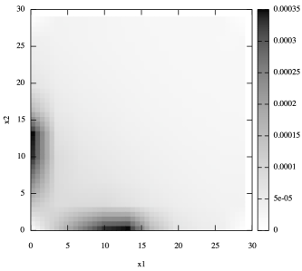
Figure 2: Difference between upper and lower bounds on states in $\mathcal{C}$ for $\epsilon=0.1$.

V Conclusion

We have demonstrated how to calculate equilibrium probability bounds of infinite MPM by combining Lyapunov theory with numerical approximation and bounding techniques. Much remains to be done with respect to implementation efficiency, since various time-space tradeoffs appear worthwhile to be explored.

References

- [1] P.-J. Courtois. Analysis of large Markovian models by parts. Applications to queueing network models. In Messung, Modellierung und Bewertung von Rechensystemen, 3. GI/NTG-Fachtagung, pages 1–10, 1985.
- [2] P.-J. Courtois and P. Semal. Bounds for the positive eigenvectors of nonnegative matrices and for their approximations by decomposition. J. ACM, 31(4):804–825, 1984.
- [3] F. Didier, T. A. Henzinger, M. Mateescu, and V. Wolf. Fast adaptive uniformization of the chemical master equation. In Proc. of HIBI, 2009. To appear.
- [4] P. W. Glynn and A. Zeevi. Bounding stationary expectations of Markov processes. Ethier, Stewart N. (ed.) et al., Markov processes and related topics: A Festschrift for Thomas G. Kurtz. Selected papers of the conference, Madison, WI, USA, July 10–13, 2006. Beachwood, OH: IMS, Institute of Mathematical Statistics. Institute of Mathematical Statistics Collections 4, 195-214., 2008.
- [5] M. Hegland, C. Burden, L. Santoso, S. Macnamara, and H. Booth. A solver for the stochastic master equation applied to gene regulatory networks. J. Comput. Appl. Math., 205:708–724, 2007.
- [6] T. Jahnke and W. Huisinga. Solving the chemical master equation for monomolecular reaction systems analytically. Journal of Mathematical Biology, 54:1–26, 2007.
- [7] T. G. Kurtz. The relationship between stochastic and deterministic models for chemical reactions. J. Chem. Phys., 57(7):2976 –2978, 1972.
- [8] A. Loinger, A. Lipshtat, N. Q. Balaban, and O. Biham. Stochastic simulations of genetic switch systems. Phys. Rev. E, 75(2):021904, 2007.
- [9] C. D. Meyer. Stochastic complementation, uncoupling Markov chains, and the theory of nearly reducible systems. SIAM Rev., 31(2):240–272, 1989.
- [10] J. Paulsson. Summing up the noise in gene networks. Nature, 427(6973):415–418, 2004.
- [11] R. Sidje, K. Burrage, and S. MacNamara. Inexact uniformization method for computing transient distributions of Markov chains. SIAM J. Sci. Comput., 29(6):2562–2580, 2007.
- [12] P. S. Swain, M. B. Elowitz, and E. D. Siggia. Intrinsic and extrinsic contributions to stochasticity in gene expression. Proceedings of the National Academy of Science, USA, 99(20):12795–12800, 2002.
- [13] M. Thattai and A. van Oudenaarden. Intrinsic noise in gene regulatory networks. PNAS, USA, 98(15):8614–8619, July 2001.
- [14] R. Tweedie. Sufficient conditions for regularity, recurrence and ergodicity of Markov processes. Math. Proc. Camb. Phil. Soc., 78:125–130, 1975.