Effects of walls

Abstract

We analyze here the energy states and associated wave functions available to a particle acted upon by a delta function potential of arbitrary strength and sign and fixed anywhere within a one-dimensional infinite well. We consider how the allowed energies vary with the well’s width and with the location of the delta function within it. The model subtly distinguishes between whether the delta function is located at rational or irrational fractions of the well’s width: in the former case all possible energy eigenvalues are solutions to a straightforward dispersion relation, but in the later case, to make up a complete set these ‘ordinary’ solutions must be augmented by the addition of ‘nodal’ states which vanish at the delta function and so do not ‘see’ it. Thus, although the model is a simple one, due to its singular nature it needs a little careful analysis. The model, of course, can be thought of as a limit of more physical smooth potentials which, though readily succumbing to straightforward numerical computation, would give little generic information.
PACS numbers: 03.65.-w, 73.21.Fg, 01.40.-d

I Introduction

Calculating the energy states for the motion of a particle in a ‘simple’ one dimensional infinite square well finds its way into all standard quantum mechanics texts. But because the potential representing the walls is sharp and infinite the model has subtleties. For instance a consistent definition of a momentum operator for it is challenging dubin1 ; garcia . Another intriguing property of the infinite well is that for certain initial states the time development of the spatial probability density can show fractal behavior berry1 . There is also the topic of wave packet revival in such a well rob ; styer . And the time dependence of a particle’s wave function in a suddenly expanded well can show interesting features aslangul . Clearly, when sharp edges and infinities are involved, care is important.

In this paper we compound the singularity by adding within the well a fixed delta function potential of arbitrary sign, strength and location. For this model, due to the containing walls, all solutions to the Schrödinger equation are bound states, but the model does have its niceties. We find for instance that although, as expected for the bound states of any one-dimensional system, all of its energy eigen-states are non-degenerate, should the delta function be located at a rational fraction of the well’s width, then a subset of these energies approach in the limit of strong attraction or repulsion, double degeneracy.

In addition to examining several other properties and limits of the model we have computed—for both attraction and repulsion— the ground state energy of the system as a function of the location of the delta function. For the case of attraction this energy has a minimum when the force center is located at the center of the well. For a wide box this minimum is nearly flat, but it becomes sharper when the well width is reduced to sizes of order of the spatial decay length characterizing the ‘molecular’ size of the bound state of an attractive delta function in free space.

The model has not, of course, escaped attention. Patil patil and Atkinson and Crater atkinson give analyses for the case that the delta function potential is located precisely at the center of the well. Bera and his co-workers bera place it anywhere within the well and utilize perturbation theory. Joglekar jog computes the energy eigenvalues when it is located at irrational multiples of the well’s width and considers weak and strong coupling limits. Epstein epstein uses the well with the delta function located at the center in order to gain insight into the interesting question posed by Wigner wigner1 as to whether the energy levels of a hydrogen atom should be derivable from second order perturbation theory in view of the fact that it is known to be proportional to the fourth power of the electron charge and therefore to the square of the Coulomb interaction.

We were motivated to consider the model by the long standing problem of the effects of containment on molecule states and energies dating back to work by Michels michels , Sommerfeld sommerfeld and their co-workers, in the early heyday of quantum mechanics, applying approximations to study what might be said to be the canonical problem—that of a hydrogen atom with its nucleus fixed at the center of an impenetrable sphere. Other more recent papers discuss this model with various methods of approximation. See for instance references varshni1 ; varshni2 ; yngve ; goldman ; goodfriend and, especially froeman which includes a short review of work on this model up to 1987. More recently Changa and co-workers changa have applied perturbation theory to estimate the energies when the hydrogen nucleus is shifted from the center of the the spherical box.

The particular advantage of the model we consider here is that no approximations are necessary to discuss the energy levels and their dependence either on the well width or on the location of the force center. It would be gratifying to be able to do the same with other model interactions. For instance one might try a ‘one dimensional Coulomb’ repulsion or attraction, $v(x)\sim 1/|x|$, $x\neq 0$. But it is a sobering fact that even with no walls present, so that $x$ is any real number bar zero, there seems to be no final agreement for that model as to the available energy levels and corresponding eigenstates loudon ; andrews ; xdd ; nouri ; a a .

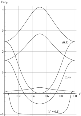
Figure 2: The result of numerical calculations (for values $(0.1,0.4,0.5)$ of the parameter $f=\Lambda/L$) for the dependence of the ‘Relative Energy’ $E/E_{B}$ of the lowest energy eigenvalue versus $\rho=\ell/L$ locating the delta function within a box of side $L$. The curves with minima are for an attractive potential $(\lambda>0)$. Their partner curves, with maxima, correspond to a repulsive interaction of the same strength. The energy of the single bound state of an attractive potential of strength $|\lambda|$ is $E=-E_{B}$, Eq. (8), and $\Lambda$ is the spatial decay length for that state, Eq. (7).

The paper is arranged as follows. We give the general solution in Sec. II. Its nature depends upon whether the ratio $\ell/L$ is a rational or irrational number, where $\ell$ is the delta function’s position within a well of width $L$. When that ratio is irrational all solutions are straightforward ‘ordinary’ solutions, but when it is rational a complete set of solutions includes both the ordinary ones together with those we choose to call ‘nodal’ solutions. For both cases we confirm in Sec. III mutual orthogonality between all solutions corresponding to different energies. In Secs. IV and V we consider the limits of weak and strong coupling for any location of the delta function potential within the well. In taking these limits, when $\ell/L$ is rational care must be exercised to include both the nodal and ordinary solutions. In Sec. VI we discuss solutions for the special symmetric case that the delta function is located precisely in the middle of the well, for which $\ell/L$ is the rational number $1/2$. In Sec. VII we consider in some detail the ground state of the model, especially with respect to its energy dependence on the relative location $\ell/L$, for various signs and strengths of the delta function potential. This is plotted in Fig. 2.

II solution

A particle of mass $m$ free to move within a one-dimensional well with sides at $x=0$ and $x=L$ has energy eigenstates

$$\psi^{(0)}_{N}(x)=\sqrt{\frac{2}{L}}\,\sin\left(\frac{N\pi x}{L}\right),\quad N=1,2,3,\ldots\,,$$ (1)

and corresponding energies

$$E^{(0)}_{N}=\frac{\hbar^{2}}{2m}\left(\frac{N\pi}{L}\right)^{2}.$$ (2)

For odd values of $N$ these states are symmetric about the middle ($x=L/2$) while those for even $N$ are antisymmetric.

A particle constrained by no walls but acted upon by a one-dimensional delta function potential located at $x=\ell$, namely

$$v(x)=-\lambda\delta(x-\ell),$$ (3)

has the associated Schrödinger equation

$$-\frac{\hbar^{2}}{2m}\Psi^{\prime\prime}(x)-\lambda\delta(x-\ell)\Psi(x)=E\Psi(x).$$ (4)

where, if $\Psi_{-}$ and $\Psi_{+}$ are solutions to the left ($x<\ell$) and right ($x>\ell$) of the delta function, the conditions to be satisfied at the potential are

$$-\frac{\hbar^{2}}{2m}\left(\Psi^{\prime}_{+}(\ell)-\Psi^{\prime}_{-}(\ell)\right)=\lambda\Psi_{-}(\ell)\quad{\rm and}\quad\Psi_{-}(\ell)=\Psi_{+}(\ell).$$ (5)

For an attractive interaction ($\lambda>0$) the single bound state is represented by

$$\Psi_{\ell}\,(x)=\frac{1}{\sqrt{\Lambda}}\,{\rm exp}\left({-\frac{|x-\ell|}{\Lambda}}\right),$$ (6)

where

$$\Lambda\equiv\frac{\hbar^{2}}{m\lambda}$$ (7)

is a measure of the ‘size’ of the bound state and the energy is

$$-E_{B}\equiv-\frac{m\lambda^{2}}{2\hbar^{2}}=-\frac{\hbar^{2}}{2m}\frac{1}{\Lambda^{2}}.$$ (8)

Whichever the sign of $\lambda$, solutions to (4) also include a continuum of positive energy unbound states, the scattering states.

Now consider putting the potential (3) inside a box of finite side $L$. Then all states of the system are bound under the combined action of the walls and delta function. For this model, solutions must satisfy Eq. (4), must vanish at the walls and must obey conditions (5). For $x\neq\ell$ solutions of Eqs. (3) and (4) are linear combinations of ${\rm exp}(\pm{\rm i}kx)$, with energy $E=\hbar^{2}k^{2}/2m$. To be continuous at $x=\ell$ and vanish at $x=0$ and $x=L$ solutions will have the form

$$\psi(x)=\begin{cases}\psi_{+}(x)=C\sin(k(L-x))\sin(k\ell)&\text{for $\ell\leq x\leq L$}\\ \psi_{-}(x)=C\sin(kx)\sin(k(L-\ell))&\text{for $0\leq x\leq\ell$},\end{cases}$$ (9)

where $C$ is a constant which may depend on $k$, $L$ and $\ell$.

Applying the first of boundary conditions (5) gives the energy dispersion relation. It is

$$k\Lambda\sin(kL)=2\sin(k\ell)\sin(k(L-\ell)),$$ (10)

where $\Lambda$ is given by (7). One set of solutions to (10) is given by

$$\sin(kL)=0,\quad\quad\sin(k\ell)=0,\quad\quad\sin(k(L-\ell))=0,$$ (11)

where any one of these equations implies the other two. Here $k$ must meet the two-fold condition

$$k=\frac{\pi n}{L}=\frac{\pi p}{\ell}\quad\mbox{so that}\quad\frac{\ell}{L}=\frac{p}{n},$$ (12)

where $n$ and $p$ are positive integers. We shall assume that the ratio $p/n$ has been reduced to its primitive form—that is to say with no common factors other than unity—so that, because $\ell/L=p/n=pj/(nj)$, we can write all of these nodal solutions $\psi^{(\textbf{n})}$, and their energies, for any such given value of $\ell/L$ as

$$\psi_{n,\,j}^{(\textbf{n})}(x)=\sqrt{\frac{2}{L}}\sin\left(\frac{nj\,\pi x}{L}\right)\,\,\mbox{and}\,\,\,\,E_{n,\,j}=\frac{\hbar^{2}}{2m}\left(\frac{nj\,\pi}{L}\right)^{2},\quad j=1,2,3\ldots,$$ (13)

with wave numbers given by

$$kL=jn\pi.$$ (14)

The particular feature of these solutions is that they have nodes at the location of the delta function potential. They are that subset of the standing wave solutions (1) for a free particle in a well with this property. Because they vanish at $x=\ell$ they satisfy both conditions (5). As an example, when $\ell/L$ equals $1/3$ (or $2/3$) the states are $\psi_{3,\,j}^{(\textbf{n})}(x)=\sqrt{2/L}\,\sin(3\pi jx/L)$ with energies $E_{3,j}=(\hbar^{2}/2m)(3\pi j/L)^{2}$ where $j=1,2,3\ldots$.

When $\sin(kL)$ does not vanish Eq. (10) can be re-expressed as

$$k\Lambda=kL\left(\frac{\Lambda}{L}\right)=\frac{2\sin(k\ell)\sin(k(L-\ell))}{\sin(kL)},$$ (15)

or, equivalently, as

$$\frac{kL}{2}\left(\frac{2\Lambda}{L}\right)=\tan\left(\frac{kL}{2}\right)-2\frac{\sin^{2}\left(\frac{kL}{2}\mu\right)}{\sin(kL)}\quad\mbox{where}\quad\mu=2\frac{\ell}{L}-1\,$$ (16)

and $\ell$ varies from $0$ to $L$ as $\mu$ ranges from $-1$ to $1$. We choose to call solutions for $k$ to either of these versions of the dispersion relation (together with their associated wave functions) ordinary solutions.

Should $\ell/L$ be a rational number, complete information about the nodal states and their energies (all positive) are given by Eqs. (13) and (14). The ordinary states exist for all values of $\ell$ between $0$ and $L$, with energies $E=\hbar^{2}k^{2}/(2m)$. For positive energies the allowed values of $k$ are real-valued. In that case, solutions for $kL$ to Eq. (15) occur at intersections with the expression on the right-hand side of a straight line passing through the origin with slope $(\Lambda/L)$. Similar comments apply to Eq. (16) in terms of $kL/2$ and slope $2\Lambda/L$. For negative energies, should there be any, the wave number is $k={\rm i}\kappa$, where $\kappa$ is real. In that case the energy is $E=-\hbar^{2}\kappa^{2}/(2m)$ and, letting $k\rightarrow{\rm i}\kappa$ in the pair (15) and (16) and in (9), one must solve either of the equations

$$\kappa L\left(\frac{\Lambda}{L}\right)=\frac{2\sinh(\kappa\ell)\sinh(\kappa(L-\ell))}{\sinh(\kappa L)}=\tanh\left(\frac{\kappa L}{2}\right)-2\frac{\sinh^{2}\left(\frac{\kappa L}{2}\mu\right)}{\sinh(\kappa L)},$$ (17)

with corresponding wave functions

$$\psi(x)=\begin{cases}D\sinh(\kappa(L-x))\sinh(\kappa\ell)&\text{for $\ell\leq x\leq L$}\\ D\sinh(\kappa x)\sinh(\kappa(L-\ell))&\text{for $0\leq x\leq\ell$}\,.\end{cases}$$ (18)

III orthogonality

We choose to confirm by direct calculation that for this one-dimensional problem all solutions corresponding to different energies are, as expected, mutually orthogonal.

Note first that, because the nodal solutions are free particle states in a simple well, it follows at once that those for different energies are mutually orthogonal. Then too these nodal solutions, Eq. (13), are orthogonal to the ordinary states. To see this, write the nodal states in condensed notation as

$$\psi^{({\textbf{n}})}(x)=\sqrt{\frac{2}{L}}\sin(\nu x),\quad\mbox{where}\quad\nu=\frac{nj\,\pi}{L}=\frac{pj\,\pi}{\ell}.$$ (19)

Now, for $k\neq 0$ and $k\neq\nu$,

$$\int_{0}^{\ell}\sin(\nu x)\sin(kx)\,{\rm d}x=(-)^{pj}\,\frac{\nu\sin(k\ell)}{k^{2}-\nu^{2}}$$

and

$$\int_{\ell}^{L}\sin(\nu x)\sin(k(L-x))\,{\rm d}x=-(-)^{pj}\,\frac{\nu\sin(k(L-\ell))}{k^{2}-\nu^{2}}.$$

Then using definition (9) gives

$$\int_{0}^{L}\psi(x)\psi^{({\textbf{n}})}(x)\,{\rm d}x=\int_{0}^{\ell}\psi_{-}(x)\psi^{({\textbf{n}})}(x)\,{\rm}dx+\int_{\ell}^{L}\psi_{+}(x)\psi^{({\textbf{n}})}(x)\,{\rm}dx=0.$$ (20)

Orthogonality also holds between any $\psi^{(\textbf{n})}$ and any ordinary solution $\psi$ with negative energies $E=-\hbar^{2}\kappa^{2}/(2m)$, where $\kappa$ is a solution to equation (17).

Finally, the ordinary solutions (9), where $k$ satisfies the dispersion relation (15), are orthogonal to each other for different values of $k$. For instance, including subscripts to indicate the $k$-dependence of wave functions, $\psi_{k,\pm}(x)$ and normalization constants $C_{k}$, we find by direct calculation, that when $k\neq k^{\prime}$,

$$\int_{0}^{L}\psi_{k}(x)\psi_{k^{\prime}}(x)\,{\rm d}x = \int_{0}^{\ell}\psi_{k,-}(x)\psi_{k^{\prime},-}(x)\,{\rm d}x+\int_{\ell}^{L}\psi_{k,+}(x)\psi_{k^{\prime},+}(x)\,{\rm d}x$$

$$= \frac{C_{k}C_{k^{\prime}}}{2}(A-B),$$

where, doing the integrals and rearranging,

$$A = \frac{1}{(k-k^{\prime})}\big{[}\sin(k(L-\ell))\sin(k^{\prime}(L-\ell))\sin((k-k^{\prime})\ell)$$

$$+ \sin(k\ell)\sin(k^{\prime}\ell)\sin((k-k^{\prime})(L-\ell))\big{]}$$

$$\mbox{and}\quad B = \frac{1}{(k+k^{\prime})}\big{[}\sin(k(L-\ell))\sin(k^{\prime}(L-\ell))\sin((k+k^{\prime})\ell)$$

$$+ \sin(k\ell)\sin(k^{\prime}\ell)\sin((k+k^{\prime})(L-\ell))\big{]}.$$

Then, by using the eigenvalue equation (15) and trigonometric identities one finds that

$$A=\frac{\Lambda}{2}\sin(kL)\sin(k^{\prime}L)=B,$$

so that, when $k\neq k^{\prime}$,

$$\int_{0}^{L}\psi_{k}(x)\psi_{k^{\prime}}(x)\,{\rm d}x=0.$$ (21)

IV weak coupling

The need to include both the nodal and ordinary solutions to make up a complete set can be seen by considering the limit of weak coupling for which $|\lambda|$ is small and $|\Lambda|/L$ large. In that limit one would expect, whatever the value of $\ell\in(0,L)$, that solutions (9) and their energies would approach those of a free particle in a well, Eqs. (1) and (2), no more and no less.

Consider solutions with positive energies. For arbitrary $\ell\in(0,L)$, in addition to the nodal states—which exist only when $\ell/L$ is rational—we have the ordinary states. For them $kL/\pi$ is not an integer and the dispersion relation can be written, say, as (15). Solutions for $kL$ to either equation are intersections of a straight line passing through the origin with slope $\Lambda/L$, large positive for attraction or large negative for repulsion. These intersections occur only near any divergences of the right-hand side (RHS) of Eq. (15), i.e. near the zeroes of $\sin(kL)$. Then, setting $kL=N\pi+\epsilon$, where $\epsilon$ is small but of either sign, shows that near these zeroes we have, approximately,

$$\mbox{RHS}\simeq\begin{cases}-(2/\epsilon)\sin^{2}(N\pi\ell/L)+\sum\limits_{n\geq 0}a_{n}(N)\,\epsilon^{n}\quad(\mbox{for}\,\,N=1,2,3\ldots)\\[11.38092pt] \,\,\,\,\,(\epsilon/2)(1-\mu^{2})+b(\epsilon)\quad(\mbox{for}\,\,N=0,\,\,\epsilon<\pi),\end{cases}$$ (22)

where $b(\epsilon)$ is monotonically increasing as a function of $\epsilon$ in the interval $[0,\pi)$ and $\mu=2(\ell/L)-1$.

Suppose first that $\ell/L$ is irrational. In that case the function $\sin(N\pi\ell/L)$ doesn’t vanish for any non-zero integer $N$. Then, using the first of these two equations in (15), with $kL=N\pi+\epsilon$, gives (for $N=1,2,3,\ldots$),

$$\epsilon=-2\frac{\sin^{2}(N\pi\ell/L)}{N\pi(\Lambda/L)}+\mbox{terms in higher inverse powers of}\,\,(\Lambda/L).$$

Using the second of equations (22) in (15) verifies that there is no solution in this limit for $N=0$. To summarize: when $\ell/L$ is irrational, solutions for $kL$ to (15)—or, what is equivalent, (16)—will, for ever weaker coupling ($|\Lambda|/L\rightarrow\infty$), approach $N\pi$ for attraction or repulsion, where $N=1,2,3\ldots$, so making up the full set of energies for a free particle in a well. Also, it is easy to see, in the limit $kL=N\pi+\epsilon$ with $\epsilon\rightarrow 0$, that solutions (9) approach those of the free particle in a well, Eq. (1).

If instead $\ell/L$ should take the rational value $p/n$, which we assume has been reduced by eliminating all common factors, then $\sin(N\pi\ell/L)$ will vanish when and only when $N=j\,n$, $j=1,2,3\ldots$. There are in the limit, therefore, no ordinary solutions for these values of $N$, but we do have the nodal states, Eqs. (13) and (14). In addition to these nodal states, as we know from the argument just given for irrational $\ell/L$, for large $|\Lambda|/L$ there exist ordinary solutions for all other integral values of $N$ again making up the full set of solutions for a free particle in a one-dimensional well.

For negative energies, similar arguments show that when $|\Lambda|/L$ is large there are no solutions to either of Eqs. (17).

V strong coupling

Now consider, for any $\ell\in(0,L)$, the strong coupling limit, for which the magnitude of $\Lambda/L$ is small. Graphical argument shows that in this case, and only for attraction ($\lambda>0$), there is a single state of negative energy. This is easily verified by considering Eq. (17) for small positive $\Lambda/L$. For any value of $\mu$ between $-1$ and $+1$ the right-hand side of that equation is positive and monotonically increasing as a function of positive $\kappa L$, from zero asymptotically to the value +1. Thus, the single solution approaches the value $\kappa\Lambda=1$, giving the limiting energy value $E=-\hbar^{2}\kappa^{2}/(2m)=-E_{B}$.

Except for the single bound state when the potential is attractive, for strong coupling the behavior of the oscillatory positive energy solutions to Eq. (4) is controlled to some extent by the product $\lambda\,\psi(\ell)$ in the potential energy term, for which one expects that whatever its sign, as the magnitude of $\lambda$ increases any ordinary solution evaluated at the potential, $\psi(\ell)$, will decrease in compensation. Of course when $\ell/L$ is rational, the corresponding nodal solutions strictly vanish at the delta function and so are independent of the magnitude of $\lambda$, so long as it is non-zero.

For the positive energies, when $|\Lambda|/L$ is small, we can say, from equation (10), that $\sin(k\ell)\sin(k(L-\ell))$ is also small, so that, whatever the sign of $\lambda$,

$$\mbox{either (a)}\quad k\ell=n_{1}\pi+\varepsilon_{1}\quad\quad\mbox{or (b)}\quad k(L-\ell)=n_{2}\pi+\varepsilon_{2},$$ (23)

where $n_{1}$ and $n_{2}$ are any positive integers and $\varepsilon_{1}$ and $\varepsilon_{2}$ are small and vanish as $|\Lambda|/L\rightarrow 0$. Note that, in the limits of vanishing $\varepsilon_{1}$ and $\varepsilon_{2}$, cases (a) and (b) cannot both hold, for then, according to (9), the wave function would strictly vanish.

Suppose first that $\ell/L$ is irrational. Then the two cases given in (23) generate, in the limit, distinct energies and do not overlap for any values of $n_{1}$ and $n_{2}$: If this were not so, then for some integers $n_{1}$ and $n_{2}$ we would have $kL=n_{1}\pi$ and $k(L-\ell)=n_{2}\pi$ for the same value of $k$ so that $\ell/L$ would be rational.

Cases (a) and (b) of (23) give, in the limit of vanishing $\Lambda/L$, nothing other than the energy levels of a free particle in separate wells of width $\ell$ and $(L-\ell)$. We can underline this by deriving the wave functions in the strong coupling limit. For case (a), using in Eq. (9) the first of expressions (23) and taking the limit $\varepsilon_{1}\rightarrow 0$, gives

$$\psi(x)\rightarrow\begin{cases}0\quad\mbox{for}\quad\ell\leq x\leq L\\ \sqrt{2/\ell}\,\sin(n_{1}\pi x/\ell)\quad\mbox{for}\quad 0\leq x\leq\ell.\end{cases}$$

And, similarly, for case (b): in the limit $\varepsilon_{2}\rightarrow 0$ these states approach the ordinary well states constrained to the interval $[\ell,L]$ with quantum number $n_{2}$. That the energies approach those of free particle motion in separate wells of widths $\ell$ and $L-\ell$ as $|\Lambda|/L\rightarrow 0$ (when $\ell/L$ is an irrational number) has been pointed out by Joglekar jog .

There are subtleties when $\ell/L$ is rational, with $\ell/L=p/n$, where we assume as usual that all common factors have been eliminated from numerator and denominator. In that case, for all values of $\Lambda$, we have the nodal solutions, Eqs. (13) and (14), with wave numbers given by $kL=jn\pi$, where $j=1,2,3\cdots.$ And, as before, in addition to those we have the ordinary solutions for which $\sin(k\ell)\sin(k(L-\ell))$ is small. For these, from Eq. (23),

$$\mbox{either (a)}\quad kL=n_{1}\pi\,(n/p)+\varepsilon_{a}\quad\quad\mbox{or (b)}\quad kL=n_{2}\pi\,n/(n-p)+\varepsilon_{b},$$ (24)

where $\varepsilon_{a}$ and $\varepsilon_{b}$ are small. In this case possibilities (a) and (b) are both satisfied whenever $n_{2}/n_{1}=(n-p)/p\,.$ But that instance gives—as we have said—a vanishing wave function and so must be ruled out as a solution. Another property is that when $n_{1}=jp$ or $n_{2}=(n-p)j$, where $j=1,2,3\cdots$, they are converging to nodal state energies. But note that, however small $|\Lambda|/L$ may be, so long as it is non-zero these ordinary states are distinct from nodal states and orthogonal to them. In summary: when $\ell/L=p/n$ (reduced) then the set of limiting values for $kL$ as $|\Lambda|/L$ approaches zero comprises the nodal values together with all distinct (non-duplicating) limits in Eq. (24).

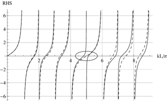
Figure 1: This shows the right-hand side (RHS) of Eq. (15) as a function of $kL$ in units of $\pi$ for $\ell/L=2/5$ (dashed) and $\ell/L=0.415$ (solid). Solutions for the ordinary states are intersections of the curves with a straight line from the origin having slope $\pi\Lambda/L$. When $\ell/L=2/5$ the lowest nodal state has a wave number given by $kL/\pi=5$, which is shared with an ordinary state (dashed line) in the limit $|\Lambda|\rightarrow 0$. That the dashed curve moves from the value $5$ shows that this limiting degeneracy is lifted as $|\Lambda|$ moves from zero. On the other hand, note that even when $\Lambda=0$ this double degeneracy is lifted by moving the potential away from the value $2/5$. The fact that $0.415=83/200$ is also rational does not effect this basic splitting: Its lowest lying nodal state occurs well to the right, at $kL/\pi=200$.

As an example we have considered the case $\ell/L=2/5$. Its nodal states have wave vectors given by $kL/\pi=5j$, $j=1,2,3,\ldots$. In addition to these we have the ordinary states. In the limit $|\Lambda|/L\rightarrow 0$ these are given by the zeroes of the right-hand side (RHS) of Eq. (15) (and (16)) with $\ell/L=2/5$. This is shown as the dashed lines in Fig. 1 as a function of $kL/\pi$ for values up to $kL/\pi=9$. The solid curves show the same function plotted for the nearby value $\ell/L=0.415=83/200$. Solutions for $kL/\pi$ in equation (15) occur at intersections of the curves with a straight line through the origin with slope $\Lambda\pi/L$. Thus the figure shows that in the limit $|\Lambda|/L\rightarrow 0$ the degeneracy between the ordinary state and the lowest nodal energy at $kL/\pi=5$ is lifted by moving the potential. It also shows that, with $\ell/L=2/5$ for example, the double degeneracy at $kL/\pi=5$ (that occurs in the limit $|\Lambda|/L\rightarrow 0$) is split when $\Lambda/L$ is nonzero and of either sign. The zeroes of the functions shown in Fig. 1 can easily be computed from Eq. (24).

To explore the rational case $\ell/L=2/5$ a bit further we have calculated the lowest energy eigenfunction that is doubly degenerate in the limit $|\Lambda|/L\rightarrow 0$. The lowest energy nodal state is, from (13), given by $\psi_{5,1}^{(\textbf{n})}(x)=\sqrt{2/L}\sin(5\pi x/L)$. To get the ordinary solution at this energy we let $kL=5\pi+\varepsilon$ in Eq. (9) and take the limit to find

$$\psi(x)=\begin{cases}\quad D\sin(5\pi x/L)\quad\mbox{for}\quad(2/5)L\leq x\leq L\\ -(3/2)D\sin(5\pi x/L)\quad\mbox{for}\quad 0\leq x\leq(2/5)L,\end{cases}$$

where $D=2/(\sqrt{3L})$ is a normalization constant. In the limit this ordinary solution vanishes at the delta function $(x=2L/5)$, suffers a discontinuity of slope there, and is orthogonal to the nodal solution $\psi_{5,1}^{(\textbf{n})}$.

VI the special case $\ell=1/2$

The simplest choice is to locate the delta potential precisely in the middle so that $\ell/L$ is the rational number $1/2$ and $\mu=0$. For this symmetric case it turns out that the ordinary and nodal states are precisely equal in number in the sense that their energies interleave. That is not the case for all other choices of $\ell/L$, where the symmetry is lost, but it is still true that both types are countably infinite in number and that their inclusion is necessary to make up a complete set.

The nodal wave functions and their energies, $\psi_{2,\,j}^{(\textbf{n})}(x)$ and $E_{2,j}$, are given by (13) with wave vectors $kL=2j\,\pi$, $j=1,2,3\ldots$, Eq. (14). These energies $E_{2,j}$ are, of course, all positive.

For the ordinary solutions any negative energy eigenvalue would have $k={\rm i}\kappa$ and $E=-\hbar^{2}\kappa^{2}/(2m)$ where, putting $\mu=0$ in (17), $\kappa$ would satisfy the equation $(\kappa L/2)(2\Lambda/L)=\tanh(\kappa L/2)$. A sketch of this equation with respect to the variable $x=\kappa L/2$ shows that there are no solutions for $\kappa$ when the interaction is a repulsion, none for relatively weak attraction ($1<2\Lambda/L$), and but a single solution for relatively strong attraction ($0<2\Lambda/L<1$). In particular in the limit of very strong binding, for which $2\Lambda/L$ approaches zero from above, $\kappa\rightarrow 1/\Lambda$, and the energy approaches $-E_{B}$.

For the ordinary solutions at positive energies, acceptable values for $kL$ must, from (16), obey the equation $(kL/2)(2\Lambda/L)=\tan(kL/2)$. This will include all the ordinary solutions except when the potential is relatively strongly attractive, for which $0<2\Lambda/L<1$ and the lowest energy moves to negative values.

When the interaction is repulsive or relatively weakly attractive all ordinary states have positive energies, and a sketch reveals that, for this symmetric case, these solutions for $kL$ interleave between those for the nodal solutions. In this sense, for the special case $\ell=1/2$ the nodal and ordinary states are equal in number.

For a strong attraction ($0<2\Lambda/L<1$) there is but one negative energy state (18). If the potential is repulsive, whatever its strength, then all states have positive energies. In addition to the nodal states $\psi_{2,\,j}^{(\textbf{n})}(x)$ we have the ordinary states. Of these, should there be attraction, there will be, as $\Lambda/L\rightarrow 0^{+}$, the single negative energy state with energy $-E_{B}$ and wave function approaching $\Psi_{L/2}$, where (see Eq. (6))

$$\Psi_{L/2}(x)=\frac{1}{\sqrt{\Lambda}}\,{\rm exp}\left({-\frac{|x-L/2|}{\Lambda}}\right)\quad\mbox{for}\quad 0<x<L.$$

For strong repulsion (and for strong attraction apart from the ground state $\Psi_{L/2}$) all states have positive energies $E=\hbar^{2}k^{2}/(2m)$. For these states $|\Lambda|/L$ is small and solutions for $kL$ are in the neighborhood of the zeroes of $\tan\left(kL/2\right)$, namely $kL=2j\pi+\varepsilon$, where $\varepsilon$ approaches zero as $|\Lambda|/L\rightarrow 0$ and $j=1,2,3\ldots$. Thus, as $|\Lambda|/L\rightarrow 0$, the energies of these ordinary states converge towards a double degeneracy with each and every one of the the nodal state values $E_{2,j}$,   Eq. (13), except, for attraction, the lowest state.

It is easy to find the positive energy wave functions for strong interaction. From (13) the nodal states are $\psi_{2,\,j}^{(\textbf{n})}(x)=\sqrt{2/L}\,\sin\left(2j\pi x/L\right)$. Using $kL=2j\pi+\varepsilon$ in Eq. (9), taking the limit $\varepsilon\rightarrow 0$ and normalizing, gives the following expression for the ordinary states in the limit of strong interaction:

$$\psi_{j}(x)=\theta(x-(L/2))\,\psi_{2,\,j}^{(\textbf{n})}(x)\quad(j=1,2,3\ldots),$$

where $\theta$ is the step function

$$\theta(u)=\begin{cases}+1\quad u>0\\ -1\quad u<0\,.\end{cases}$$ (25)

These ordinary states have a discontinuous slope at the delta function, are even valued with respect to reflection about $x=L/2$ and are manifestly orthogonal to the nodal states which are odd valued about the middle. In this limit the energy of each ordinary state $\psi_{j}(x)$ approaches that of the corresponding nodal state $\psi_{2,\,j}^{(\textbf{n})}(x)$: in this case of high symmetry all states approach doubly degeneracy in the limit of strong interaction. However we note that for all finite strengths of the contact potential all energies of this one-dimensional system are, of course, non-degenerate.

VII ground state

We considered in subsection VI solutions to Eqs. (16) and (17) with $\mu=0$, i.e. the case $\ell=L/2$. In that instance the ground state energy is positive for all strengths of repulsion, $\Lambda<0$, and also for relatively weak attraction, $2\Lambda/L>1$. But for relatively strong binding, for which the inequality $1>2\Lambda/L>0$ holds, the ground state energy is negative. And, in particular, in the limit of strong binding, when $\Lambda/L\rightarrow 0^{+}$, it approaches $-\hbar^{2}/(2m\Lambda^{2})=-E_{B}$, the bound state energy of the free system, Eq. (8).

When the force center is not in the middle, then $\mu$ does not vanish and a re-analysis is required. For that case, whatever the details may be, we can say from the start that for either sign and any magnitude of $\Lambda$, because Eqs. (16) and (17) are symmetric with respect to $\mu$ about $\mu=0$, as a function of $\ell$, any ordinary state energy eigenvalue must be symmetric about $\ell=L/2$. It is easy to see from (13) that this symmetry also applies to the nodal states.

Consider, in particular, configurations with the delta function located near to the left wall, say, with $\ell=\epsilon$, where $\epsilon$ is small and positive. As $\epsilon$ decreases, the nodal solution energy eigenvalues— see Eq. (13)—will rapidly increase to large positive values. To see this, note that with $\ell/L=p/n$, $n$ must increase without bound as $\epsilon\rightarrow 0^{+}$, taking with it the accompanying energies $E_{n,j}\sim(j\,n)^{2}$, $j=1,2,3,\cdots$.

As for the ordinary solutions, with $\ell=\epsilon$ and $\epsilon\rightarrow 0^{+}$, we can say that as the delta function approaches a wall there are no negative energies. To see this, expand Eq. (17) for small $\epsilon$ to get $\tanh(\kappa L)/(\kappa L)\simeq-2\epsilon^{2}/(\Lambda L)$. In the limit $\epsilon\rightarrow 0^{+}$ this has no solutions for any finite value of $\kappa$. So all energy eigenvalues are non-negative when the delta function potential is near to either wall.

For arbitrary $\mu\in(-1,1)$, a sketch allows us to predict the existence of ordinary solutions for small positive and negative energies, the transition between which occurs at $k=0$. The second of Eqs. (22) (which applies when $kL$ is small) and the graphical picture suggests the following: that for small $kL$ and an attractive potential ($\Lambda>0$) there is a solution for small real valued $kL$ provided the slope $\Lambda/L$ is greater than $(1-\mu^{2})/2$; that $k$ vanishes when $\Lambda/L=(1-\mu^{2})/2$; that there is a negative energy solution with $k={\rm i}\kappa$ when $\Lambda/L$ is less than $(1-\mu^{2})/2$. From Eq. (16) $\mu=2\ell/L-1$, so we can say that as a function of $\ell/L$, the ground state energy passes through zero when $\Lambda/L=[1-\mu^{2}]/2=2(1-\ell/L)\ell/L$, or

$$\ell/L=(1/2)\left(1\pm\sqrt{1-2\Lambda/L}\right).$$ (26)

Note that, because $\ell/L$ is restricted to the interval $(0,1)$, there can only be zeroes of energy provided $0<2\Lambda/L<1$, i.e. for relatively strong attraction.

Finally, consider the ordinary solutions for values of $\ell$ near, say, the left wall so that $\ell=\epsilon$, where $\epsilon$ is small. Expanding Eq. (15) to lowest order and collecting terms gives $\tan(kL)/(kL)\simeq-2\epsilon^{2}/\Lambda L$, so that in the limit $\epsilon\rightarrow 0$, $kL\rightarrow N\pi$ $(N=1,2,\cdots)$, or $E\rightarrow\hbar^{2}N^{2}\pi^{2}/(2mL^{2})$. Thus, in this limit the energies approach those of a free particle in a well, Eq. (2). To see how this limit is approached as $\ell\rightarrow 0^{+}$ we can set $kL=N\pi+\Delta$, where $\Delta$ is small. Then $\tan(kL)/kL=\tan\Delta/(N\pi+\Delta)\simeq\Delta/(N\pi)$, so that $\Delta/(N\pi)\simeq-2\epsilon^{2}/(\Lambda L)$ or $\Delta\simeq-2N\pi\epsilon^{2}/(\Lambda L)$. The corresponding energy is

$$E=\frac{\hbar^{2}}{2mL^{2}}(N\pi+\Delta)^{2}\simeq\frac{\hbar^{2}}{2m}\left(\frac{N\pi}{L}\right)^{2}\left(1-\frac{4\epsilon^{2}}{L\Lambda}\right),\quad N=1,2,3\cdots.$$ (27)

This result holds for either sign of $\Lambda=\hbar^{2}/(m\lambda)$. The conclusion, then, is that when the delta function is near either wall, as a function of distance away, the energies are parabolic in form with zero slope at the wall, and they are a local maximum (minimum) for an attractive (repulsive) interaction.

The lowest, ground state, energy corresponds to the choice $N=1$ in Eq. (27). Numerical calculation gives the dependence of energy eigenvalues on $\ell$ as it is varied from $0$ to $L$. All energies above the ground state are positive so for them one must solve either of the pair (15) or (16). For the ground state, when $2\Lambda/L>1$, these equations pertain, but when $2\Lambda/L<1$ Eq. (17) holds. Their solutions join smoothly at zero energy, for which $k$ vanishes. This happens at values of $\ell$ given by Eq. (26). Results for the ground state are shown in Fig. 2 where the ratio $E/E_{B}$ versus $R=\ell/L$ is plotted for the three values $(0.1,0.4,0.5)$ for the parameter $f=\Lambda/L$. We have done this for attractive and repulsive delta function potentials having the same strength $|\Lambda|$. For the former (latter) case $\Lambda>0$ ($\Lambda<0$) and the the energy eigenvalues have their minimum (maximum) value at $f=1/2$.

Generally, for the case of attraction, should the wall separation $L$ increase to values large with respect to the characteristic length $\Lambda$ one expects that the ground state energy would approach $-E_{B}$, Eq. (8). Indeed in the limit $\kappa L\rightarrow\infty$ Eq. (17) becomes $\kappa\rightarrow 1$, provided $0<\ell<L$ so that $\kappa\rightarrow 1/\Lambda$ and $E\rightarrow-\hbar^{2}/(2m\Lambda^{2})=-E_{B}$. Note, however, that however large $L$ may be, according to Eq. (27) with $n=1$, in the limits $\ell\rightarrow 0^{+}$ and $\ell\rightarrow L^{-}$ the wall dominates so that the energy approaches $\hbar^{2}\pi^{2}/(2mL^{2})$, the lowest energy of a free particle in the well. This is consistent with Fig. 2. In the other extreme of small $L$, the walls dominate, whatever the value of $\ell$. In this limit $|\Lambda|/L$ is large, which is equivalent to weak coupling. For this limit the analysis around the first of Eqs. (22) shows that $kL\rightarrow\pi$ as $|\Lambda|/L\rightarrow\infty$, so that in the limit $L\rightarrow 0$ we find that $E\rightarrow\hbar^{2}\pi^{2}/(2mL^{2})=\pi^{2}f^{2}E_{B}$, the lowest energy of a free particle in a well.

VIII concluding remarks

The model analyzed here is simple and exactly solvable, but we are unaware of any complete published analysis. If we think of an attractive delta function as a very simple model of the nucleus of a relatively massive atom, then along the lines of the Born-Oppenheimer approximation we might suppose that its position $\ell\in(0,L)$ can be varied as a parameter. Thus the model suggests, reasonably, that for an attractive interaction the configuration of lowest energy is for the ‘nucleus’ to avoid the walls. This agrees with the perturbation calculations of Changa et al changa for hydrogen in a hard spherical cavity. Note that as the well width is decreased the uncertainty principle demands that eventually the kinetic energy term of the Schrödinger equation is the dominant contribution to the energy. As we pointed out in Sec. VII this also applies for a well of any width should the fixed potential be located sufficiently close to either wall.

We have shown that the energy levels and wave functions for choice $\ell=L/2$ follow as the limit of a ‘top hat’ model potential having height $H$ and width $W<L$ where the ‘area’ $HW$ is held constant and $W\rightarrow 0^{+}$, and it is reasonable to conjecture that the same result applies for off-center top hat potentials and, more generally, to any sequence of model potentials which approaches the delta function as a limit.

As a limit of sequences of non-singular potentials, the choice $v(x)=-\lambda\delta(x-\ell)$ does require care in its handling. In particular the behavior of the nodal energies, Eqs. (13) and (14), is somewhat chaotic as $\ell$ is varied. For instance, for any given ‘rational’ position $\ell/L=p/n$, the lowest nodal energy is proportional to $n^{2}$, so that the lowest such energies occur, in increasing order, at relative position $\ell/L=1/2$ and then at $\ell/L=(1/3,1/4,1/5,\cdots)$ to the left of the midpoint or, symmetrically, at points $\ell/L=(2/3,3/4,4/5,\cdots)$ to its right. But should $\ell/L$ be moved through nodal points arbitrarily close to any one of these points then the lowest associated energy sweeps through chaotically large, even infinite, values. Nevertheless, we emphasize that, for rational values of $\ell/L$ a complete set of solutions requires both the nodal and ordinary ones. By contrast, the ordinary solutions have energies which are solutions to Eqs. (15) or (16). They are smooth continuous functions of position $\ell\in(0,L)$. For instance this is true for the ground state discussed in Sect. VII.

To conclude the paper we should like to make a few remarks of a purely mathematical nature concerning the model, most of which remains to be done. First we prove that the Hamiltonian, properly defined mathematically, is self adjoint. As the reader will know, self adjointness is that subtle property of a symmetric (hermitian) operator that guarantees that the operator can be exponentiated. For the Hamiltonian, this condition is necessary and sufficient to guarantee a unique time translation group. For our formal Hamiltonian, which we here denote

$$S=-\frac{\hbar^{2}}{2m}\,\frac{d^{2}}{dx^{2}}-\lambda\delta(x-\ell),$$

the process begins by defining a domain of definition for its interpretation as a sesquilinear form. We choose as domain $\mathcal{D}$ the set of functions $f\in L^{2}(0,L)$ in the Hilbert space which belong to the domain of the kinetic operator and, in addition, have a first derivative $f^{\prime}$ which satisfies the discontinuity boundary condition at $x=\ell$. This implies that $f^{\prime}\in L^{2}(0,L)$. We can then consider the form

$${\mbox{{[}{[}}}\,g\,,\,f\,{\mbox{{]}{]}}}:=\int_{0}^{L}\makebox[0.0pt][l]{\rule[7.5pt]{16.51738pt}{0.4pt}}g(t)\,[Sf](t)\,dt$$

for all $f$ in the domain $\mathcal{D}$. By a simple calculation, involving no more than integration by parts, it follows that the associated quadratic form is lower bounded,

$${\mbox{{[}{[}}}\,f\,,\,f\,{\mbox{{]}{]}}}=\frac{\hbar^{2}}{2m}\lVert f^{\prime}\rVert^{2}-\lambda\lvert f(\ell)\rvert^{2}\,\geq-\lambda\,\sup_{0\leq x\leq L}|f(x)|^{2}\,>-\infty\,.$$ (28)

It is now standard that the form can be extended to a closed form which defines a self adjoint operator, the Friedrichs extension of $S$. It is this extension that we take as the mathematically proper Hamiltonian $H$. For details of the extension we recommend Davies EBD1 and §124 of Riesz and Sz.-Nagy RN .

This leaves the following to prove: the spectrum of $H$ consists only of eigenvalues, indeed of those eigenvalues we have obtained earlier and only those. We firmly believe these to be true, and that, in consequence, for a given $\ell$ and $\lambda$ the eigenfunctions we obtained constitute an orthonormal basis for $L^{2}(0,L)$. We remark that were we to independently prove that the eigenfunctions were complete then the eigenvalues we found would comprise the spectrum of $H$.

Figures

References

- (1) D. A. Dubin, J. Kiukas, and J-P Pellonpää “Momentum Observables for a Bounded Interval” (article in preparation) (2010).
- (2) P. L. Garcia de Leon, J. P. Gazeau, and J. Queva “Infinite quantum well: A coherent state approach,” Phys. Lett. A 372, 3597–3607 (2008).
- (3) M. V. Berry, “Quantum fractals in boxes,” J. Phys. A: Math. Gen. 29, 6617–6629 (1996).
- (4) R. W. Robinett, “Quantum wave packet revivals,” Physics Reports 392, 1–119 (2004).
- (5) D. F. Styer, “Quantum revivals versus classical periodicity in the infinite square well,” Am. J. Phys. 69, 56–62 (2001).
- (6) C. Aslangul, “Surprises in the suddenly-expanded infinite well,” J. Phys. A: Math. Theor. 41, 075301-1-23 (2008).
- (7) S. H. Patil, “Completeness of the energy eigenfunctions for the one-dimensional -function potential,” Am. J. Phys. 68 712-714 (2000).
- (8) D. A. Atkinson and H. W. Crater, “An exact treatment of the Dirac delta function potential in the Schrödinger equation,” Am. J. Phys. 43 301-304 (1975).
- (9) N. Bera, K. Bhattacharyya and J. K. Bhattacharjee, “Perturbative and nonperturbative studies with the delta function potential,” Am. J. Phys. 76 250-257 (2008).
- (10) Y. N. Joglekar, “Particle in a box with a -function potential: strong and weak coupling limits,” Am. J. Phys. 77 734-736 (2009).
- (11) S. T. Epstein, “Application of the Rayleigh-Schrödinger Perturbation Theory to the Delta Function Potential,” Am. J. Phys. 28 495-496 (1960).
- (12) E. P. Wigner, “Application of the Rayleigh-Schrödinger Perturbation Theory to the Hydrogen Atom,” Phys. Rev. 94 77-78 (1954).
- (13) A. Michels, J. De Boer, and A. Bijl, “Remarks concerning molecular interaction and their influence on polarizability,” Physica 4 981-994 (1937).
- (14) A. Sommerfeld and H. Welker, “Künstliche Grenzbedingungen beim Keplerproblem,” Annalen der Physik 32 56-65 (1938).
- (15) Y. P. Varshni, “Accurate wavefunctions for the confined hydrogen atom at high pressures,” J. Phys. B:At. Mol. Opt. Phys. 30 L589593 (1997).
- (16) Y. P. Varshni, “Critical cage radii for the confined hydrogen atom,” J. Phys. B:At. Mol. Opt. Phys. 31 2849-2856 (1998).
- (17) S. Yngve, “The energy levels and the corresponding normalized wave functions for a model of a compressed atom. II,” J. Math. Phys. 29 931-936 (1988).
- (18) S. Goldman and C. Joslin, “Spectroscopic Properties of an Istropically Compressed Hydrogen Atom,” J. Chem. Phys. 96 6021-6027 (1992).
- (19) P. L. Goodfriend, “On the use of linear variation basis functions that do not satisfy the boundary conditions” J. Phys. B:At. Mol. Opt. Phys. 23 1373-1379 (1990).
- (20) P. O. Fröman, S. Yngve and N. Fröman, “The energy levels and the corresponding normalized wave functions for a model of a compressed atom,” J. Math. Phys. 28 1813-1826 (1987).
- (21) M. E. Changa, A. V. Scherbinin, and V. I. Pupyshev, “Perturbation theory for the hydrogen atom in a spherical cavity with off-centre nucleus” J. Phys. B:At. Mol. Opt. Phys. 33 421-432 (2000).
- (22) R. Loudon, “One-Dimensional Hydrogen Atom,” Am. J. Phys. 27 649-655 (1959).
- (23) M. Andrews, “Ground State of the One-Dimensional Hydrogen Atom,” Am. J. Phys. 34 1194-1195 (1966).
- (24) Dai Xianxi, Jixin Dai and Jiqiong Dai, “Orthogonality criteria for singular states and the nonexistence of stationary states with even parity for the one-dimensional hydrogen atom,” Phys. Rev. A 55 2617-2624 (1997).
- (25) S. Nouri, “Generalized coherent states for the Coulomb problem in one dimension,” Phys. Rev. A 65 062108-1-5 (2002).
- (26) G. Abramovici and Y. Avishai, “The one-dimensional Coulomb problem,” J. Phys. A:Math. Theor. 42 285302-1-29 (2009).
- (27) E. B. Davies, Spectral Theory and Differential Operators. Cambridge University Press, 1995.
- (28) F. Riesz and B. Sz.-Nagy, Functional Analysis, F. Ungar, New York 1955.