Bose-Einstein condensation at finite momentum and magnon condensation in thin film ferromagnets

Abstract

We use the Gross-Pitaevskii equation to determine the spatial structure of the condensate density of interacting bosons whose energy dispersion $\epsilon_{\bm{k}}$ has two degenerate minima at finite wave-vectors $\pm\bm{q}$. We show that in general the Fourier transform of the condensate density has finite amplitudes for all integer multiples of $\bm{q}$. If the interaction is such that many Fourier components contribute, the Bose condensate is localized at the sites of a one-dimensional lattice with spacing $2\pi/|\bm{q}|$; in this case Bose-Einstein condensation resembles the transition from a liquid to a crystalline solid. We use our results to investigate the spatial structure of the Bose condensate formed by magnons in thin films of ferromagnets with dipole-dipole interactions.

1 Introduction

This work is motivated by the recent discovery Demokritov06 ; Demidov07 ; Dzyapko07 ; Demidov08 ; Demokritov08 of a new coherence phenomenon of magnons in thin stripes made of the magnetic insulator yttrium-iron garnet (YIG). The energy dispersion $\epsilon_{\bm{k}}$ of the lowest magnon mode in this system has a rather unusual momentum-dependence which is crucial to understand the experiments: for a certain range of orientations of an external magnetic field, $\epsilon_{\bm{k}}$ exhibits two degenerate minima at finite wave-vectors $+\bm{q}$ and $-\bm{q}$. The value of $\bm{q}$ is determined by a subtle interplay between exchange interactions, dipole-dipole interactions, and finite-size effects Kalinikos86 ; Kreisel09 . The experimentally observed strong enhancement of the occupation of the magnon modes with wave-vectors $\pm\bm{q}$ has been interpreted as Bose-Einstein condensation (BEC) of magnons.

Another class of boson systems where the energy dispersion has degenerate minima at finite wave-vectors $\pm{\bm{q}}$ are magnon gases in quantum helimagnets in a magnetic field Ueda09 . Apart from the experimental relevance, the general problem of BEC in systems where the energy dispersion has a minimum for non-zero wave-vectors is interesting on its own. In this context we mention the work by Yukalov Yukalov78 , who has investigated BEC in an interacting Bose system whose energy dispersion is minimal on a sphere in momentum space. He found that in this case the condensed state neither exhibits off-diagonal long-range nor is it superfluid. Moreover, Yukalov also pointed out an interesting analogy between BEC at finite momentum and the liquid-crystal phase transition, which can also be understood in terms of a Ginzburg-Landau functional whose Gaussian term exhibits minima on a surface in momentum space Alexander78 ; Anderson84 .

The fact that BEC of quasi-particles is not necessarily accompanied by superfluidity has been emphasized by Kohn and Sherrington Kohn70 , who classified bosons into two different types: the first type consists of bound complexes of an even number of fermions; in the case of condensation of these bosons, superfluidity and off diagonal long-range order occurs. The second type of bosons consists of quasi-particles such as excitons and magnons; when the second type condenses, there is no superfluidity, but a change of spatial or magnetic order Kohn70 ; superfluidity . Obviously, BEC of magnons in YIG is of the second type. From the point of view of critical phenomena it is not surprising that BEC at finite momentum is rather different from BEC at zero momentum. In fact, phase transitions which are characterized by an order parameter which condenses on a surface in momentum space belong to their own universality class, the so-called Brazovskii universality class Brazovskii75 ; Hohenberg95 .

In this work we shall examine the general problem of BEC in a Bose gas whose energy dispersion has degenerate minima at two finite wave-vectors $\pm\bm{q}$. We show that in this case the time-independent Gross-Pitaevskii equation implies that the Fourier transform $\phi_{\bm{k}}$ of the condensate wave-function has finite amplitudes $\phi_{0},\phi_{\pm\bm{q}},\phi_{\pm 2\bm{q}},\ldots$ for integer multiples of the fundamental wave-vector $\bm{q}$. Previously a theoretical analysis of magnon-BEC in YIG has been performed by Tupitsyn, Stamp, and Burin Tupitsyn08 . However, the effect of the spatial structure of the condensate wave-function as implied by the Gross-Pitaevskii equation was not considered by these authors.

2 BEC at finite momentum

In this section we shall study BEC in a general class of interacting boson models on a lattice whose Hamiltonian is of the form

$$H=H_{2}+H_{3}+H_{4}.$$ (1)

The quadratic part $H_{2}$ of the Hamiltonian is given by

$$H_{2}=\sum_{\bm{k}}\left[\epsilon_{\bm{k}}a^{\dagger}_{\bm{k}}a_{\bm{k}}+\frac{\gamma_{\bm{k}}}{2}a^{\dagger}_{\bm{k}}a^{\dagger}_{-\bm{k}}+\frac{\gamma^{\ast}_{\bm{k}}}{2}a_{-\bm{k}}a_{\bm{k}}\right],$$ (2)

where $a_{\bm{k}}$ and $a^{\dagger}_{\bm{k}}$ are the usual canonical annihilation and creation operators, the energy dispersion $\epsilon_{\bm{k}}$ is assumed to exhibit two degenerate minima at finite wave-vectors $\pm\bm{q}$, and the terms proportional to the complex parameter $\gamma_{\bm{k}}$ explicitly break the $U(1)$ symmetry associated with particle number conservation. In YIG these terms are related to an external pumping filed, as explained in the appendix. In the absence of $U(1)$ symmetry, the Hamiltonian can also contain contributions involving three powers of boson operators, which in general are of the form

$$H_{3} = \frac{1}{\sqrt{N}}\sum_{\bm{k}_{1}\bm{k}_{2}\bm{k}_{3}}\delta_{\bm{k}_{1}+\bm{k}_{2}+\bm{k}_{3},0}\Bigr{[}$$ (3)

$$\frac{1}{2}\Gamma^{\bar{a}aa}_{1;23}a^{\dagger}_{-1}a_{2}a_{3}+\frac{1}{2}\Gamma^{\bar{a}\bar{a}a}_{12;3}a^{\dagger}_{-1}a^{\dagger}_{-2}a_{3}$$

$$+ \frac{1}{3!}\Gamma^{aaa}_{123}a_{1}a_{2}a_{3}+\frac{1}{3!}\Gamma^{\bar{a}\bar{a}\bar{a}}_{123}a^{\dagger}_{-1}a^{\dagger}_{-2}a^{\dagger}_{-3}\Bigr{]},$$

where $N$ is the total number of sites of the underlying lattice. For simplicity we write $a_{1}\equiv a_{\bm{k}_{1}}$ and abbreviate the interaction vertices by $\Gamma^{\bar{a}aa}_{\bm{k}_{1};\bm{k}_{2}\bm{k}_{3}}\equiv\Gamma^{\bar{a}aa}_{1;23}$ etc.. Finally, the part $H_{4}$ to the Hamiltonian involving four powers of the boson operators is in the absence of $U(1)$-symmetry given by

$$H_{4} = \frac{1}{N}\sum_{\bm{k}_{1}\ldots\bm{k}_{4}}\delta_{\bm{k}_{1}+\ldots+\bm{k}_{4},0}\Bigr{[}\frac{1}{(2!)^{2}}\Gamma^{\bar{a}\bar{a}aa}_{12;34}a^{\dagger}_{-1}a^{\dagger}_{-2}a_{3}a_{4}$$ (4)

$$+ \frac{1}{3!}\Gamma^{\bar{a}aaa}_{1;234}a^{\dagger}_{-1}a_{2}a_{3}a_{4}+\frac{1}{3!}\Gamma^{\bar{a}\bar{a}\bar{a}a}_{123;4}a^{\dagger}_{-1}a^{\dagger}_{-2}a^{\dagger}_{-3}a_{4}$$

$$+ \frac{1}{4!}\Gamma^{aaaa}_{1234}a_{1}a_{2}a_{3}a_{4}+\frac{1}{4!}\Gamma^{\bar{a}\bar{a}\bar{a}\bar{a}}_{1234}a^{\dagger}_{-1}a^{\dagger}_{-2}a^{\dagger}_{-3}a^{\dagger}_{-4}\Bigr{]}.\hskip 19.91692pt$$

In the appendix we shall show how to obtain a boson Hamiltonian of the above form from an effective spin Hamiltonian describing the lowest magnon band of YIG in the so-called parallel pumping geometry Kreisel09 ; Tupitsyn08 ; Kloss10 .

The spatial dependence of the Bose condensate is determined by the Gross-Pitaevskii equation Pitaevskii03 , which can be obtained from the extremum of the corresponding Euclidean action. In order to write the various interaction processes in a compact notation, we introduce a two-component complex field $\Phi^{\sigma}_{\bm{k}}(\tau)$, where $\tau$ is the imaginary time and $\sigma=a,\bar{a}$ labels the two components according to the prescription

$$a_{\bm{k}}\rightarrow\Phi^{a}_{\bm{k}}(\tau)\;\;,\;\;a^{\dagger}_{\bm{k}}\rightarrow\Phi^{\bar{a}}_{-\bm{k}}(\tau).$$ (5)

The quadratic part $H_{2}$ of the Hamiltonian corresponds then to the Gaussian action

$$S_{2}[\Phi] = \frac{1}{2}\int_{0}^{\beta}d\tau\sum_{\bm{k}}(\Phi^{\bar{a}}_{-\bm{k}},\Phi^{a}_{-\bm{k}})$$ (10)

$$\times \left(\begin{array}[]{cc}\partial_{\tau}+\epsilon_{\bm{k}}-\mu&\gamma_{\bm{k}}\\ \gamma_{\bm{k}}^{\ast}&-\partial_{\tau}+\epsilon_{\bm{k}}-\mu\end{array}\right)\left(\begin{array}[]{c}\Phi^{a}_{\bm{k}}\\ \Phi^{\bar{a}}_{\bm{k}}\end{array}\right),\hskip 19.91692pt$$

where $\beta$ is the inverse temperature and $\mu$ is the chemical potential. The Euclidean action corresponding to the interaction parts $H_{3}$ and $H_{4}$ can be written in the following symmetrized form,

$$S_{3}[\Phi] = \int_{0}^{\beta}d\tau\frac{1}{\sqrt{N}}\sum_{\bm{k}_{1}\bm{k}_{2}\bm{k}_{3}}\sum_{\sigma_{1}\sigma_{2}\sigma_{3}}\delta_{\bm{k}_{1}+\bm{k}_{2}+\bm{k}_{3},0}$$ (11)

$$\times\frac{1}{3!}\Gamma_{3}(\bm{k}_{1}\sigma_{1},\bm{k}_{2}\sigma_{2},\bm{k}_{3}\sigma_{3})\Phi^{\sigma_{1}}_{\bm{k}_{1}}\Phi^{\sigma_{2}}_{\bm{k}_{2}}\Phi^{\sigma_{3}}_{\bm{k}_{3}},$$

$$S_{4}[\Phi] = \int_{0}^{\beta}d\tau\frac{1}{N}\sum_{\bm{k}_{1}\ldots\bm{k}_{4}}\sum_{\sigma_{1}\ldots\sigma_{4}}\delta_{\bm{k}_{1}+\ldots+\bm{k}_{4},0}$$ (12)

$$\times\frac{1}{4!}\Gamma_{4}(\bm{k}_{1}\sigma_{1},\ldots,\bm{k}_{4}\sigma_{4})\Phi^{\sigma_{1}}_{\bm{k}_{1}}\ldots\Phi^{\sigma_{4}}_{\bm{k}_{4}},$$

where the flavor indices $\sigma_{i}=a,\bar{a}$ keep track of the two different field types, and the vertices $\Gamma_{3}(\bm{k}_{1}\sigma_{1},\bm{k}_{2}\sigma_{2},\bm{k}_{3}\sigma_{3})$ and $\Gamma_{4}(\bm{k}_{1}\sigma_{1},\ldots,\bm{k}_{4}\sigma_{4})$ are completely symmetric under the permutation of all indices. The combinatorial factors in these expressions are chosen Schuetz05 such that for a given ordering of the indices the completely symmetrized vertices can be identified with the partially symmetrized vertices appearing in Eqs. (3, 4), for example

$$\Gamma_{3}(\bm{k}_{1}\bar{a},\bm{k}_{2}a,\bm{k}_{3}a)=\Gamma^{\bar{a}aa}_{1;23}.$$ (13)

In the presence of a Bose condensate some of the expectation values $\phi_{\bm{k}}^{\sigma}=\langle\Phi_{\bm{k}}^{\sigma}\rangle$ are finite and proportional to $\sqrt{N}$. In equilibrium the order parameter fields $\phi_{\bm{k}}^{\sigma}$ are independent of the imaginary time. It is then useful to shift the integration variables $\Phi$ in the Euclidean functional integral according to $\Phi_{\bm{k}}^{\sigma}(\tau)=\phi_{\bm{k}}^{\sigma}+\delta\Phi_{\bm{k}}^{\sigma}(\tau)$ and expand the Euclidean action $S[\Phi]=S_{2}[\Phi]+S_{3}[\Phi]+S_{4}[\Phi]$ in powers of the fluctuations,

$$S[\phi+\delta\Phi]=S[\phi]+\int_{0}^{\beta}d\tau\sum_{\bm{k}\sigma}\left.\frac{\delta S[\Phi]}{\delta\Phi_{\bm{k}}^{\sigma}(\tau)}\right|_{\Phi=\phi}\delta\Phi_{\bm{k}}^{\sigma}(\tau)+\ldots.$$ (14)

The physical order parameter field is determined by demanding that the first variation of the action vanishes, which yields the Gross-Pitaevskii equation

$$0 = \left.\frac{\delta S[\Phi]}{\delta\Phi_{\bm{k}}^{\sigma}(\tau)}\right|_{\Phi=\phi}=(\epsilon_{\bm{k}}-\mu)\phi^{\bar{\sigma}}_{-\bm{k}}+\gamma_{\bm{k}}^{\sigma}\phi^{{\sigma}}_{-\bm{k}}$$ (15)

$$+ \frac{1}{\sqrt{N}}\sum_{\bm{k}_{1}\bm{k}_{2}}\sum_{\sigma_{1}\sigma_{2}}\delta_{\bm{k}+\bm{k}_{1}+\bm{k}_{2},0}$$

$$\times\frac{1}{2}\Gamma_{3}(\bm{k}\sigma,\bm{k}_{1}\sigma_{1},\bm{k}_{2}\sigma_{2})\phi^{\sigma_{1}}_{\bm{k}_{1}}\phi^{\sigma_{2}}_{\bm{k}_{2}}$$

$$+ \frac{1}{N}\sum_{\bm{k}_{1}\bm{k}_{2}\bm{k}_{3}}\sum_{\sigma_{1}\sigma_{2}\sigma_{3}}\delta_{\bm{k}+\bm{k}_{1}+\bm{k}_{2}+\bm{k}_{3},0}$$

$$\times\frac{1}{3!}\Gamma_{4}(\bm{k}\sigma,\bm{k}_{1}\sigma_{1},\bm{k}_{2}\sigma_{2},\bm{k}_{3}\sigma_{3})\phi^{\sigma_{1}}_{\bm{k}_{1}}\phi_{\bm{k}_{2}}^{\sigma_{2}}\phi^{\sigma_{3}}_{\bm{k}_{3}},\hskip 19.91692pt$$

where we have defined $\gamma_{\bm{k}}^{a}=\gamma_{\bm{k}}^{\ast}$ and $\gamma_{\bm{k}}^{\bar{a}}=\gamma_{\bm{k}}$.

To begin with, let us assume that the system condenses in a state where only the $\bm{k}=0$ mode is macroscopically occupied. Such a state tends to be favored if the dispersion has a minimum at $\bm{k}=0$. In this case

$$\phi^{\sigma}_{\bm{k}}=\delta_{\bm{k},0}\sqrt{N}\psi^{\sigma}_{0},$$ (16)

where the complex parameter $\psi^{a}_{0}=(\psi^{\bar{a}}_{0})^{\ast}$ is expected to be of the order of unity. Assuming for simplicity that $\gamma_{0}^{\sigma}=\gamma_{0}$ is real, we then obtain from our general Gross-Pitaevskii equation (15)

$$0 = r_{0}\psi^{\bar{\sigma}}_{0}+\gamma_{0}\psi^{{\sigma}}_{0}+\frac{1}{2}\sum_{\sigma_{1}\sigma_{2}}\Gamma_{3}(0\sigma,0\sigma_{1},0\sigma_{2})\psi^{\sigma_{1}}_{0}\psi^{\sigma_{2}}_{0}$$ (17)

$$+ \frac{1}{3!}\sum_{\sigma_{1}\sigma_{2}\sigma_{3}}\Gamma_{4}(0\sigma,0\sigma_{1},0\sigma_{2},0\sigma_{3})\psi^{\sigma_{1}}_{0}\psi_{0}^{\sigma_{2}}\psi^{\sigma_{3}}_{0},\hskip 19.91692pt$$

where

$$r_{0}=\epsilon_{0}-\mu.$$ (18)

We adopt here the standard notation in the field of critical phenomena Ma76 where a negative value of $r_{0}$ implies a finite expectation value of the order parameter field. Assuming further that the three-legged vertices vanish and that only the particle number conserving four-legged vertex $\Gamma^{\bar{a}\bar{a}aa}_{00;00}\equiv u_{4}$ is finite and positive, we find that the Gross-Pitaevskii equation (17) has two degenerate solutions

$$\psi_{0}^{\sigma}=\pm i\sqrt{\frac{2(\gamma_{0}-r_{0})}{u_{4}}}.$$ (19)

Note that even for positive $r_{0}=\epsilon_{0}-\mu$ the condensate is stable if the energy scale $\gamma_{0}$ associated with explicit symmetry breaking is sufficiently large. Of course, for $\gamma_{0}\neq 0$ there is no spontaneous symmetry breaking so that there is no gapless Goldstone mode in the condensed state. Due to the symmetry breaking terms $a^{\dagger}_{\bm{k}}a^{\dagger}_{-\bm{k}}$ and $a_{-\bm{k}}a_{\bm{k}}$ in the quadratic part $H_{2}$ of our Hamiltonian the effective potential

$$U_{\rm eff}[\psi_{0}^{\bar{a}},\psi_{0}^{a}]=N^{-1}S[\Phi_{\bm{k}}^{\sigma}\rightarrow\sqrt{N}\delta_{\bm{k},0}\psi_{0}^{\sigma}]$$ (20)

has two degenerate minima at purely imaginary values of the field as shown in Fig. 1. Cubic terms (which are neglected in these plots) distort the effective potential and break the degeneracy of the two minima.

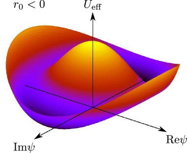
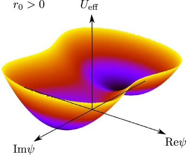
Figure 1: (Color online) Effective potential for zero momentum BEC in the presence of explicit symmetry breaking, see Eq. (20). The quadratic part of the Hamiltonian is then given by Eq. (2), where for simplicity we assume that $\gamma_{0}$ is real and positive. For the graphs the cubic vertices have been neglected and only the particle-number conserving component of the four-point vertices $\Gamma^{\bar{a}\bar{a}aa}_{00;00}\equiv u_{4}$ has been retained. The graphs are for $\gamma_{0}-r_{0}>0$ where the effective potential has two degenerate minima on the imaginary axis. Upper graph: for $r_{0}<0$ the center of the effective potential is a local maximum so that its shape resembles Napoleon’s hat. Lower graph: for $r_{0}>0$ the local maximum in (a) transforms into a saddle point.

The problem of BEC at zero momentum in the presence of $U(1)$ symmetry breaking terms has been discussed previously in Ref. DellAmore09 .

Next let us study the more interesting case where the dispersion $\epsilon_{\bm{k}}$ has two degenerate minima at finite wave-vectors $\pm{\bm{q}}$. At the first sight it seems that in this case one can find solutions of the Gross-Pitaevskii equation (15) where only the modes with $\bm{k}=\pm\bm{q}$ condense,

$$\phi^{\sigma}_{\bm{k}}=\sqrt{N}[\delta_{\bm{k},\bm{q}}\psi^{\sigma}_{1}+\delta_{\bm{k},-\bm{q}}\psi^{\sigma}_{-1}].$$ (21)

Keeping in mind that $\psi_{1}^{a}=\langle a_{\bm{q}}\rangle/\sqrt{N}$ and $\psi_{-1}^{\bar{a}}=\langle a^{\dagger}_{\bm{q}}\rangle/\sqrt{N}$, we see that $(\psi^{{\sigma}}_{1})^{\ast}=\psi^{\bar{\sigma}}_{-1}$. In real space the condensate wave-function (21) corresponds to

$$\phi^{\sigma}(\bm{r})=\frac{1}{\sqrt{N}}\sum_{\bm{k}}e^{i\bm{k}\cdot\bm{r}}\phi_{\bm{k}}^{\sigma}=e^{i{\bm{q}}\cdot{\bm{r}}}\psi_{1}^{\sigma}+e^{-i{\bm{q}}\cdot{\bm{r}}}\psi_{-1}^{\sigma}.$$ (22)

Setting $\psi_{1}^{\sigma}=\psi_{-1}^{\sigma}=\psi$, the corresponding condensate density is

$$\rho_{1}(\bm{r})=|\phi^{{a}}(\bm{r})|^{2}=4|\psi|^{2}\cos^{2}(\bm{q}\cdot\bm{r}).$$ (23)

The important point is now that a condensate wave-function of this type does not solve the Gross-Pitaevskii equation (15), because the interaction terms couple the Fourier components with $\bm{k}=\pm\bm{q}$ to all other Fourier components involving arbitrary integer multiples $n\bm{q}$ of the fundamental wave-vector $\bm{q}$, where $n=0,\pm 1,\pm 2,\ldots$. To see this more clearly, let us substitute the general ansatz

$$\phi^{\sigma}_{\bm{k}}=\sqrt{N}\sum_{n=-\infty}^{\infty}\delta_{\bm{k},\bm{q}_{n}}\psi^{\sigma}_{n}$$ (24)

into Eq. (15) where $\bm{q}_{n}=n\bm{q}$. Setting the external wave-vector $\bm{k}=-\bm{q}_{n}$ in Eq. (15) and defining $r_{n}=\epsilon_{-\bm{q}_{n}}-\mu$ and $\gamma_{n}=\gamma_{-\bm{q}_{n}}$ (assuming again that $\gamma_{\bm{k}}$ is real), we obtain the discrete Gross-Pitaevskii equation,

$$-r_{n}\psi_{n}^{\bar{\sigma}}-\gamma_{n}\psi_{n}^{\sigma} = \frac{1}{2}\sum_{n_{1}n_{2}}\sum_{\sigma_{1}\sigma_{2}}\delta_{n,n_{1}+n_{2}}V_{nn_{1}n_{2}}^{\sigma\sigma_{1}\sigma_{2}}\;\psi^{\sigma_{1}}_{n_{1}}\psi^{\sigma_{2}}_{n_{2}}$$ (25)

$$+\frac{1}{3!}\sum_{n_{1}n_{2}n_{3}}\sum_{\sigma_{1}\sigma_{2}\sigma_{3}}\delta_{n,n_{1}+n_{2}+n_{3}}U_{nn_{1}n_{2}n_{3}}^{\sigma\sigma_{1}\sigma_{2}\sigma_{3}}\;\psi^{\sigma_{1}}_{n_{1}}\psi^{\sigma_{2}}_{n_{2}}\psi^{\sigma_{3}}_{n_{3}},$$

where

$$V_{nn_{1}n_{2}}^{\sigma\sigma_{1}\sigma_{2}} = \Gamma_{3}(\bm{q}_{n}\sigma,\bm{q}_{n_{1}}\sigma_{1},\bm{q}_{n_{2}}\sigma_{2}),$$ (26)

$$U_{nn_{1}n_{2}n_{3}}^{\sigma\sigma_{1}\sigma_{2}\sigma_{3}} = \Gamma_{4}(\bm{q}_{n}\sigma,\bm{q}_{n_{1}}\sigma_{1},\bm{q}_{n_{2}}\sigma_{2},\bm{q}_{n_{3}}\sigma_{3}).$$ (27)

The crucial point is now that if we assume on the right-hand side of Eq. (25) that only the coefficients $\psi^{\sigma_{i}}_{n_{i}}$ with $n_{i}=\pm 1$ are finite, then we find after carrying out the sum that on the left-hand side all field components $\psi_{n}^{\sigma}$ with $n=0,\pm 1,\pm 2,\pm 3$ must also be finite, so that the assumption that only the modes with wave-vector $\pm\bm{q}$ condense is not self-consistent. For general interactions where all interaction coefficients $V_{nn_{1}n_{2}}^{\sigma\sigma_{1}\sigma_{2}}$ and $U_{nn_{1}n_{2}n_{3}}^{\sigma\sigma_{1}\sigma_{2}\sigma_{3}}$ are finite, the Fourier transform of a self-consistent solution of the Gross-Pitaevskii equation must therefore have finite weight for all integer multiples of $\bm{q}$. Depending on the behavior of the interaction coefficients the spatial behavior of the condensate wave-function can look rather differently. In Sec. 3 we shall show that for YIG the cubic interaction coefficients $V_{nn_{1}n_{2}}^{\sigma\sigma_{1}\sigma_{2}}$ actually vanish identically, and that the behavior of the quartic coefficients $U_{nn_{1}n_{2}n_{3}}^{\sigma\sigma_{1}\sigma_{2}\sigma_{3}}$ is such that the component $\psi_{\pm 1}^{\sigma}$ of the condensate wave-function is much larger than the other components. In this case the spatial distribution of the condensate density is to a good approximation given by Eq. (23). On the other hand for some other types of interactions many Fourier components of the solution of the discrete Gross-Pitaevskii equation can have the same order of magnitude. In this case the condensate density is strongly localized at the sites of a one-dimensional lattice with spacing $2\pi/|\bm{q}|$. For example, if we assume that the first $m$ Fourier components are finite and equal, $\psi^{\sigma}_{n}=\psi/\sqrt{m}$ for $1\leq|n|\leq m$, then the condensate density is given by

$$\rho_{m}(\bm{r})=\left|\frac{2\psi}{\sqrt{m}}\sum_{n=1}^{m}\cos(\bm{q}_{n}\cdot\bm{r})\right|^{2}.$$ (28)

To obtain a properly normalized density, it is necessary to scale the order parameter as $\psi/\sqrt{m}$. In Fig. 2 we compare the single-component density $\rho_{1}(\bm{r})$ given in Eq. (23) with the corresponding multi-component density where the $5$ odd Fourier modes $\bm{q}_{1},\bm{q}_{3},\bm{q}_{5},\bm{q}_{7},\bm{q}_{9}$ are macroscopically occupied.

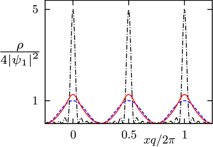
Figure 2: (Color online) This plot illustrates the fact that the condensate wave-function is more localized in real space if many Fourier components contribute. The dash-doted and the solid lines represent condensate densities associated with a condensate wave-function where the $5$ odd Fourier modes $\bm{q}_{1},\bm{q}_{3},\bm{q}_{5},\bm{q}_{7},\bm{q}_{9}$ are macroscopically occupied. For the dashed-dotted line we have assumed that all 5 modes have the same weight, while the dashed line corresponds to YIG with pumping parameter $\gamma_{1}/r_{1}=3$, see Table 1. For comparison, the dashed line is the condensate density $\rho_{1}\left(\bm{r}\right)$ where only the modes with wave vectors $\pm\bm{q}$ are macroscopically occupied, see Eq. 23.

Obviously, in this case one can already observe a strong localization of the condensate at the sites of a one-dimensional lattice with spacing $\pi/|\bm{q}|$. It is then appropriate to think of BEC as a condensation phenomenon in real space. In fact, the formation of the Bose condensate resembles in this case the phase transition from a liquid to a crystalline solid Yukalov78 . However, in the three-dimensional crystal formation problem the situation is more complicated because the Gaussian term in a Ginzburg-Landau theory exhibits a minimum on a surface in momentum space, and for the crystal structure the cubic term in the expansion of the Landau functional in powers of the density play also an important role Alexander78 ; Anderson84 .

3 BEC of magnons in YIG

It is well known Kreisel09 ; Kloss10 ; Rezende09 ; Lvov94 ; Zakharov70 ; Tsukernik75 ; Vinikovetskii79 ; Lim88 ; Kalafati89 that the effective magnon Hamiltonian for YIG can be cast into the general form given in Eqs. (1–4). In the appendix we summarize the main steps and approximations in the derivation of the magnon Hamiltonian for YIG from a realistic spin Hamiltonian and give explicit expressions for the interaction vertices. If the samples have the shape of thin stripes and if an external magnetic field is oriented along the direction of the stripes (which we call the $z$-direction), the energy dispersion $\epsilon_{\bm{k}}$ of the lowest magnon band indeed has two degenerate minima wave-vectors $\pm\bm{q}=\pm q\bm{e}_{z}$. From the explicit expressions for the three-point vertices for YIG given in Eqs. (A16, A17) and (LABEL:eq:Gammaaaa1–A34d) we see that for this direction of $\bm{q}$ all three-magnon interaction vertices $V^{\sigma\sigma_{1}\sigma_{2}}_{nn_{1}n_{2}}$ defined in Eq. (26) vanish identically, so that for the discussion of BEC in YIG one can omit the first term on the right-hand side of the discrete Gross-Pitaevskii equation (25). We can then construct self-consistent solutions of this equation involving only Fourier components $\psi_{\pm n}^{\sigma}$ with $n=(2j+1)n_{1}$, where $j=0,1,2,\ldots$, and $n_{1}$ is the label of the lowest finite Fourier component. Because in experiments the samples are kept at room temperature, leading to a finite thermal magnon density at ${\bm{k}}=\pm\bm{q}$, and energy transfer by pumping is mostly done to modes whose energy is less than $\epsilon_{2{\bm{q}}}$, we expect that the Fourier components $\psi^{\sigma}_{\pm 1}$ are dominant. In the following we therefore set $n_{1}=1$ and consider solutions of the type

$$\phi^{\sigma}_{\bm{k}}=\sqrt{N}\sum_{n\;\rm{odd}}\delta_{\bm{k},\bm{q}_{n}}\psi^{\sigma}_{n}\;.$$ (29)

The infinite set of Fourier components $\psi_{\pm 1}^{\sigma},\psi_{\pm 3}^{\sigma},\psi_{\pm 5}^{\sigma},\ldots$ is determined by setting $n=\pm 1,\pm 3,\pm 5,\ldots$ in the discrete Gross-Pitaevskii equation (25), keeping in mind that for BEC of magnons in YIG we should set $V^{\sigma\sigma_{1}\sigma_{2}}_{nn_{1}n_{2}}~{}=~{}0$ and use the four-point vertices $U_{nn_{1}n_{2}n_{3}}^{\sigma\sigma_{1}\sigma_{2}\sigma_{3}}$ defined via Eqs. (27), (A18–A20), and (A35–A35e). We have solved these equations numerically by truncating the expansion (29) at some finite order $m>|n|$. For positive $r_{1}$ non-trivial solutions can be obtained for

$$\gamma_{1}>r_{1}=\epsilon_{\bm{q}}-\mu\;.$$ (30)

If $r_{1}$ is negative, we find solutions for arbitrary $\gamma_{1}$, including $\gamma_{1}=0$. As discussed in the appendix, to describe the stationary non-equilibrium state of the magnon gas in YIG under the influence of an external microwave field oscillating with frequency $\omega_{0}$, one should re-define $\epsilon_{\bm{q}}\rightarrow\epsilon_{\bm{q}}-\omega_{0}/2$ and use an appropriate chemical potential $\mu$. It turns out that the Fourier coefficients $\psi_{n}^{\sigma}$ decay rapidly for large $n$, so that in practice it is not necessary to choose the cutoff $m$ larger than $10$ to obtain converged results. Typical numerical results are summarized in Table I and are represented graphically in Fig. 3.

Table 1: Numerical results for $\left|\psi_{1}\right|\equiv|\psi_{1}^{\sigma}|$ and the ratios $\left|\psi_{n}\right|/\left|\psi_{1}\right|$ for different values of the dimensionless pumping parameters $\gamma_{1}/r_{1}$ for $r_{1}>0$. Note that for $r_{1}>0$ there is no condensate if $\gamma_{1}/r_{1}<1$. The numbers have been obtained from the numerical solution of the discrete Gross-Pitaevskii equation (25) using realistic interaction parameters for YIG. By symmetry, for negative momenta we obtain identical results.

$\gamma_{1}/r_{1}$	$\left|\psi_{1}\right|$	$\left|\psi_{3}/\psi_{1}\right|$	$\left|\psi_{5}/\psi_{1}\right|$	$\left|\psi_{7}/\psi_{1}\right|$	$\left|\psi_{9}/\psi_{1}\right|$
$1.1$	$0.530$	$0.019$	$0.002$	$0$	$0$
$1.2$	$0.757$	$0.033$	$0.005$	$0.001$	$0$
$1.5$	$1.209$	$0.055$	$0.013$	$0.003$	$0.001$
$3.0$	$2.439$	$0.085$	$0.031$	$0.012$	$0.005$

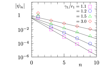
Figure 3: (Color online) Absolute values $|\psi_{n}|=\left|\psi_{n}^{\sigma}\right|$ of the Fourier components of the order parameter for BEC in YIG for different values of the dimensionless ratio $\gamma_{1}/r_{1}=\gamma_{\bm{q}}/(\epsilon_{\bm{q}}-\mu)$. The order parameter has been obtained from the numerical solution of the discrete Gross-Pitaevskii equation (25), using the fact that for YIG the three-point vertices $V^{\sigma\sigma_{1}\sigma_{2}}_{nn_{1}n_{2}}$ vanish. In this case the physically relevant solution of Eq. (25) has only odd Fourier components. Note the Fourier components $\psi_{1}^{\sigma}$ are dominant and that the higher order Fourier components $\psi_{n}^{\sigma}$ decay approximately exponentially as a function of $n$.

Obviously, for YIG the first Fourier components $\psi^{\sigma}_{\pm 1}$ of the condensate wave function are dominant, so that the spatial structure of the condensate density is to a good approximation given by $\rho_{1}(\bm{r})$ given in Eq. (23). This is consistent with the experiments by Demokritov and co-workers Demokritov06 ; Demidov07 ; Dzyapko07 ; Demidov08 ; Demokritov08 , who observed a strong enhancement of the magnon distribution only for wave-vectors $\pm\bm{q}$. Note, however, that in principle also the higher order Fourier components are finite. In fact, with increasing amplitude of the pumping field the relative weight of the higher order Fourier components also increases. For example, from our numerical data shown in Table I we see that for $\gamma_{1}/r_{1}=3$ the amplitude of the third Fourier component $\psi_{\pm 3}^{\sigma}$ is approximately $8\%$ of the amplitude of the dominant component $\psi_{\pm 1}^{\sigma}$. If the first Fourier components have the same order of magnitude and one uses realistic parameters for YIG, we estimate that the effective lattice spacing is $2\pi/|{\bm{q}}|\approx 2\cdot 10^{-7}\;\text{m}$, which is roughly a factor of 100 larger than the spacing of the underlying Bravais lattice.

4 Summary and conclusions

In summary, we have considered the general problem of BEC in an interacting Bose gas whose energy dispersion has two degenerate minima at finite wave-vectors $\pm\bm{q}$. Our main result is that for generic interactions the condensate wave-function has finite Fourier components $\psi_{n}$ for all integer multiples $\bm{q}_{n}=n\bm{q}$ of the fundamental wave-vector $\bm{q}$. For special interactions many Fourier components $\psi_{n}$ can have the same order of magnitude, so that in real space the condensate is strongly localized at the sites of a one-dimensional lattice. In this case there is a formal analogy between BEC and the liquid-solid transition.

We have also used our theory to study the condensate wave-function of the condensed magnons in the magnetic insulator yttrium-iron garnet. In this case it is appropriate to think of magnon BEC as a condensation process in momentum space, because the condensate wave-function is dominated by its leading Fourier components at $\pm{\bm{q}}$. However, if the amplitude of the oscillating external microwave field is increased, then higher order Fourier components of the condensate wave-function can be populated.

If one succeeds to extend the experiments which observe directly the magnon densities to wavevectors $k\gtrsim q$ it should be possible to detect also these higher order components. Since the order of magnitude of the higher order Fourier components drops exponentially and delocalization problems occur due to a finite slope of the dispersion away from the minimum, it is a rather challenging task to verify our prediction experimentally.

Finally, it should be mentioned that quite recently Malomed et al. Malomed10 studied the dynamics of BEC of magnons in YIG within an approach where coupled time-dependent Gross-Pitaevskii type of equations for the two components of the condensate wave-function corresponding to condensation at $\pm\bm{q}$ are written down phenomenologically. Note, however, that this approach neglects processes which couple the dominant Fourier components $\psi_{\pm 1}$ to the higher order Fourier components of the condensate wave-function.

APPENDIX: MAGNON-MAGNON INTERACTIONS IN YIG

In this appendix we outline the derivation of an effective boson Hamiltonian of the form given in Eqs. (1–4) describing the lowest magnon band of YIG, starting from the following time-dependent spin Hamiltonian, Kreisel09 ; Tupitsyn08 ; Kloss10 ; Cherepanov93 ; Rezende06 ; Rezende09

$${H}_{\rm YIG}(t) = -\frac{1}{2}\sum_{ij}\sum_{\alpha\beta}\big{[}J_{ij}\delta^{\alpha\beta}+D_{ij}^{\alpha\beta}\big{]}S_{i}^{\alpha}S_{j}^{\beta}$$ (A1)

$$-\big{[}h_{0}+h_{1}\cos(\omega_{0}t)\big{]}\sum_{i}S_{i}^{z},$$

where $\alpha,\beta=x,y,z$ label the three components of the spin operators $S^{\alpha}_{i}$, and $i,j=1,\ldots,N$ enumerate the $N$ sites $\bm{r}_{i}$ of a cubic lattice with lattice spacing $a~{}\approx~{}12.376$ Å. The exchange couplings $J_{ij}=J({\bm{r}}_{i}-{\bm{r}}_{j})$ have the value $J\approx 1.29$K if ${\bm{r}}_{i}-{\bm{r}}_{j}$ connect nearest neighbor sites and vanish otherwise. The Zeeman energy associated with a static external magnetic field $H_{e}$ is denoted by $h_{0}=\mu H_{e}$, where $\mu=g\mu_{B}$ with the Bohr magneton given by $\mu_{B}$. Setting $g=2$ we should work with an effective spin $S\approx 14.2$ as discussed in Refs. Kreisel09 ; Tupitsyn08 . The time-dependent part of Eq. (A1) represents the Zeeman energy induced by an external microwave field oscillating with frequency $\omega_{0}$. The energy scale $h_{1}$ associated with the oscillating component of the magnetic field is assumed to be small compared with $h_{0}$, so that both the static and the oscillating magnetic field point into the direction of the macroscopic magnetization, which we call the $z$-direction (parallel pumping). Finally, the matrix elements of the dipolar tensor $D_{ij}^{\alpha\beta}=D^{\alpha\beta}(\bm{r}_{i}-\bm{r}_{j})$ are

$$D_{ij}^{\alpha\beta}=(1-\delta_{ij})\frac{\mu^{2}}{|\bm{r}_{ij}|^{3}}\left[3\hat{r}_{ij}^{\alpha}\hat{r}_{ij}^{\beta}-\delta^{\alpha\beta}\right],$$ (A2)

where ${\bm{r}}_{ij}={\bm{r}}_{i}-{\bm{r}}_{j}$ and $\hat{\bm{r}}_{ij}={\bm{r}}_{ij}/|{\bm{r}}_{ij}|$.

Because the experimentally relevant YIG stripes are several thousand lattice spacings thick, we may assume that for magnetic fields oriented along the direction of the stripes the classical ground state is a saturated ferromagnet with all spins pointing in the direction of the external magnetic field. The components of the spin operators can then be expressed in terms of canonical boson operators $b_{i}$ and $b_{i}^{\dagger}$ as follows Holstein40 ,

$$S_{i}^{+} = \sqrt{2S}\sqrt{1-\frac{b^{\dagger}_{i}b_{i}}{2S}}\;b_{i}=\sqrt{2S}\left[b_{i}-\frac{b_{i}^{\dagger}b_{i}b_{i}}{4S}+\ldots\right],$$

$$S_{i}^{-} = \sqrt{2S}b_{i}^{\dagger}\sqrt{1-\frac{b^{\dagger}_{i}b_{i}}{2S}}=\sqrt{2S}\left[b_{i}^{\dagger}-\frac{b_{i}^{\dagger}b_{i}^{\dagger}b_{i}}{4S}+\ldots\right],$$

$$S_{i}^{z} = S-b_{i}^{\dagger}b_{i},$$ (A3c)

where $S_{i}^{+}=S_{i}^{x}+iS_{i}^{y}$ and $S_{i}^{-}=S_{i}^{x}-iS_{i}^{y}$. Retaining terms up to fourth order in the boson operators we obtain

$$H_{\rm YIG}(t)=H_{0}(t)+H_{2}(t)+H_{3}+H_{4}+{\cal{O}}(S^{-1/2}),$$ (A4)

where the boson-independent term and the term quadratic in the bosons are Kreisel09 ; Kloss10

$$H_{0}(t) = -\frac{S^{2}}{2}\sum_{ij}\left[J_{ij}+D^{zz}_{ij}\right]$$ (A5)

$$-NS[h_{0}+h_{1}\cos(\omega_{0}t)],$$

$${H}_{2}(t) = \sum_{ij}\left[A_{ij}b_{i}^{\dagger}b_{j}+\frac{B_{ij}}{2}\left(b_{i}b_{j}+b_{i}^{\dagger}b_{j}^{\dagger}\right)\right]$$ (A6)

$$+h_{1}\cos(\omega_{0}t)\sum_{i}b_{i}^{\dagger}b_{i},$$

with coefficients given by

$$A_{ij} = \delta_{ij}h_{e}+S(\delta_{ij}\sum_{n}J_{in}-J_{ij})$$ (A7)

$$+S\left[\delta_{ij}\sum_{n}D_{in}^{zz}-\frac{D_{ij}^{xx}+D_{ij}^{yy}}{2}\right],$$

$$B_{ij} = -\frac{S}{2}[D_{ij}^{xx}-2iD_{ij}^{xy}-D_{ij}^{yy}].$$ (A8)

The cubic contribution $H_{3}$ to the boson Hamiltonian is of order $\sqrt{S}$ and involves only the dipolar tensor,

$${H}_{3} = \sqrt{\frac{S}{2}}\sum_{ij}\Bigl{[}\left(D_{ij}^{zy}+iD_{ij}^{zx}\right)\Bigl{(}b_{i}^{\dagger}b_{j}^{\dagger}b_{j}+\frac{1}{4}b_{i}^{\dagger}b_{i}^{\dagger}b_{i}\Bigr{)}+{\rm{h.c.}}\Bigr{]}.$$

The quartic part of the boson Hamiltonian can be written as

$${H}_{4} = -\frac{1}{2}\sum_{ij}J_{ij}\Bigl{[}n_{i}n_{j}-\frac{1}{2}\left(b_{i}^{\dagger}b_{j}^{\dagger}b_{j}b_{j}+\textrm{h.c.}\right)\Bigr{]}$$

$$+ \frac{1}{2}\sum_{ij}\left(D_{ij}^{xx}+D_{ij}^{yy}\right)\Bigl{[}n_{i}n_{j}+\frac{1}{4}\left(b_{i}^{\dagger}b_{j}^{\dagger}b_{j}b_{j}+\textrm{h.c.}\right)\Bigr{]}$$

$$+ \frac{1}{4}\sum_{ij}\left[\left(D_{ij}^{xx}-2iD_{ij}^{xy}-D_{ij}^{yy}\right)b_{i}^{\dagger}b_{i}b_{i}b_{j}+\textrm{h.c.}\right],$$

where we have abbreviated $n_{i}=b^{\dagger}_{i}b_{i}$. Next, we Fourier transform the Hamiltonian to momentum space, setting

$$b_{i}=\frac{1}{\sqrt{N}}\sum_{\bm{k}}e^{i\bm{k}\cdot\bm{r}_{i}}b_{\bm{k}},$$ (A11)

where for simplicity we impose periodic boundary conditions in all directions. A more accurate calculation should take into account the finite extend in the direction where the experimentally relevant samples have the smallest extension (which we call the $x$-direction) Kreisel09 . For our purpose it is sufficient to impose periodic boundary conditions in all directions, which amounts to approximating the eigenfunctions of the exchange matrix $J_{ij}$ by plane waves. The lowest magnon band is then obtained by simply setting $k_{x}=0$. In Ref. Kreisel09 we have shown that this uniform mode approximation reproduces the qualitative features of the dispersion of the lowest magnon mode rather well. In momentum space, the quadratic part $H_{2}(t)$ of our bosonized Hamiltonian becomes

$${H}_{2} = \sum_{\bm{k}}\left[A_{\bm{k}}b_{\bm{k}}^{\dagger}b_{\bm{k}}+\frac{B_{\bm{k}}}{2}\left(b_{\bm{k}}^{\dagger}b^{\dagger}_{-\bm{k}}+b_{-\bm{k}}b_{\bm{k}}\right)\right]$$ (A12)

$$+h_{1}\cos(\omega_{0}t)\sum_{\bm{k}}b_{\bm{k}}^{\dagger}b_{\bm{k}},$$

with

$$A_{\bm{k}} = \sum_{i}e^{-i\bm{k}\cdot\bm{r}_{ij}}A_{ij},\;\;\;B_{\bm{k}}=\sum_{i}e^{-i\bm{k}\cdot\bm{r}_{ij}}B_{ij}.\hskip 19.91692pt$$ (A13)

The interaction parts can be written as

$${H}_{3} = \frac{1}{\sqrt{N}}\sum_{\bm{k}_{1}\bm{k}_{2}\bm{k}_{3}}\delta_{\bm{k}_{1}+\bm{k}_{2}+\bm{k}_{3},0}$$ (A14)

$$\times\frac{1}{2!}\Bigl{[}\Gamma_{1;23}^{\bar{b}bb}b_{-1}^{\dagger}b_{2}b_{3}+\Gamma_{12;3}^{\bar{b}\bar{b}b}b_{-1}^{\dagger}b_{-2}^{\dagger}b_{3}\Bigr{]},$$

$${H}_{4} = \frac{1}{N}\sum_{\bm{k}_{1}\dots\bm{k}_{4}}\delta_{\bm{k}_{1}+\bm{k}_{2}+\bm{k}_{3}+\bm{k}_{4},0}\Bigl{[}\frac{1}{(2!)^{2}}\Gamma_{12;34}^{\bar{b}\bar{b}bb}b_{-1}^{\dagger}b_{-2}^{\dagger}b_{3}b_{4}$$ (A15)

$$+\frac{1}{3!}\Gamma_{1;234}^{\bar{b}bbb}b_{-1}^{\dagger}b_{2}b_{3}b_{4}+\frac{1}{3!}\Gamma_{123;4}^{\bar{b}\bar{b}\bar{b}b}b_{-1}^{\dagger}b_{-2}^{\dagger}b_{-3}^{\dagger}b_{4}\Bigr{]},$$

where the properly symmetrized three-point vertices are

$$\Gamma_{1;23}^{\bar{b}bb} = \sqrt{\frac{S}{2}}\Big{[}D_{\bm{k}_{2}}^{zy}-iD_{\bm{k}_{2}}^{zx}+(\bm{k}_{2}\rightarrow\bm{k}_{3})$$ (A16)

$$\hskip 22.76219pt+\frac{1}{2}(D_{\bm{0}}^{zy}-iD_{\bm{0}}^{zx})\Big{]},$$

$$\Gamma_{12;3}^{\bar{b}\bar{b}b} = \big{(}\Gamma_{3;21}^{\bar{b}bb}\big{)}^{\ast},$$ (A17)

and the symmetrized four-point vertices are

$$\Gamma_{12;34}^{\bar{b}\bar{b}bb} = -\frac{1}{2}\Bigl{[}J_{\bm{k}_{1}+\bm{k}_{3}}+J_{\bm{k}_{2}+\bm{k}_{3}}+J_{\bm{k}_{1}+\bm{k}_{4}}+J_{\bm{k}_{2}+\bm{k}_{4}}$$ (A18)

$$\hskip 14.22636pt+D_{\bm{k}_{1}+\bm{k}_{3}}^{zz}+D_{\bm{k}_{2}+\bm{k}_{3}}^{zz}+D_{\bm{k}_{1}+\bm{k}_{4}}^{zz}+D_{\bm{k}_{2}+\bm{k}_{4}}^{zz}$$

$$\hskip 14.22636pt-\sum_{i=1}^{4}(J_{\bm{k}_{i}}-2D_{\bm{k}_{i}}^{zz})\Bigr{]},$$

$$\Gamma_{1;234}^{\bar{b}bbb} = \frac{1}{4}\Bigl{[}D_{\bm{k}_{2}}^{xx}-2iD_{\bm{k}_{2}}^{xy}-D_{\bm{k}_{2}}^{yy}$$ (A19)

$$\hskip 5.69054pt+(\bm{k}_{2}\rightarrow\bm{k}_{3})+(\bm{k}_{2}\rightarrow\bm{k}_{4})\Big{]},$$

$$\Gamma_{123;4}^{\bar{b}\bar{b}\bar{b}b} = \big{(}\Gamma_{4;123}^{\bar{b}bbb}\big{)}^{\ast}.$$ (A20)

The Fourier transforms of the exchange and dipolar couplings are defined by

$$J_{\bm{k}} = \sum_{i}e^{-i\bm{k}\cdot\bm{r}_{ij}}J_{ij},$$ (A21)

$$D_{\bm{k}}^{\alpha\beta} = \sum_{i}e^{-i\bm{k}\cdot\bm{r}_{ij}}D^{\alpha\beta}_{ij}.$$ (A22)

Finally, we use a Bogoliubov transformation to diagonalize the time-independent part of ${H}_{2}(t)$,

$$\left(\begin{array}[]{c}b_{\bm{k}}\\ b^{\dagger}_{-\bm{k}}\end{array}\right)=\left(\begin{array}[]{cc}u_{\bm{k}}&-v_{\bm{k}}\\ -v_{\bm{k}}^{\ast}&u_{\bm{k}}\end{array}\right)\left(\begin{array}[]{c}a_{\bm{k}}\\ a^{\dagger}_{-\bm{k}}\end{array}\right),$$ (A29)

where

$$u_{\bm{k}}=\sqrt{\frac{A_{\bm{k}}+\epsilon_{\bm{k}}}{2\epsilon_{\bm{k}}}}\;\;,\;\;v_{\bm{k}}=\frac{B_{\bm{k}}}{|B_{\bm{k}}|}\sqrt{\frac{A_{\bm{k}}-\epsilon_{\bm{k}}}{2\epsilon_{\bm{k}}}},$$ (A30)

and

$$\epsilon_{\bm{k}}=\sqrt{A_{\bm{k}}^{2}-|B_{\bm{k}}|^{2}}.$$ (A31)

After this transformation the quadratic part of the Hamiltonian reads Kloss10 ; Lvov94

$${H}_{2}(t) = \sum_{\bm{k}}\left[\epsilon_{\bm{k}}a^{\dagger}_{\bm{k}}a_{\bm{k}}+\frac{\epsilon_{\bm{k}}-A_{\bm{k}}}{2}\right]\hskip 85.35826pt$$ (A32)

$$+h_{1}\cos(\omega_{0}t)\sum_{\bm{k}}\left[\frac{A_{\bm{k}}}{\epsilon_{\bm{k}}}a^{\dagger}_{\bm{k}}a_{\bm{k}}+\frac{A_{\bm{k}}-\epsilon_{\bm{k}}}{2\epsilon_{\bm{k}}}\right]$$

$$+\cos(\omega_{0}t)\sum_{\bm{k}}\left[\gamma_{\bm{k}}a^{\dagger}_{\bm{k}}a^{\dagger}_{-\bm{k}}+\gamma_{\bm{k}}^{\ast}a_{-\bm{k}}a_{\bm{k}}\right],$$

where

$$\gamma_{\bm{k}}=-\frac{h_{1}B_{\bm{k}}}{2\epsilon_{\bm{k}}}.$$ (A33)

Substituting the Bogoliubov transformation (A29) into the expressions for $H_{3}$ and $H_{4}$ given in Eqs. (A14, A15), we arrive at expressions given in Eqs. (3, 4), with the cubic vertices explicitly given by

$$\Gamma_{123}^{aaa} = -\Gamma_{1;23}^{\bar{b}bb}v_{1}u_{2}u_{3}-\Gamma_{2;13}^{\bar{b}bb}v_{2}u_{1}u_{3}-\Gamma_{3;12}^{\bar{b}bb}v_{3}u_{1}u_{2}$$

$$+\Gamma_{12;3}^{\bar{b}\bar{b}b}v_{1}v_{2}u_{3}+\Gamma_{23;1}^{\bar{b}\bar{b}b}v_{2}v_{3}u_{1}+\Gamma_{13;2}^{\bar{b}\bar{b}b}v_{1}v_{3}u_{2},$$

$$\Gamma^{\bar{a}aa}_{1;2,3} = \Gamma_{1;23}^{\bar{b}bb}u_{1}u_{2}u_{3}+\Gamma_{2;13}^{\bar{b}bb}v_{1}v_{2}u_{3}+\Gamma_{3;12}^{\bar{b}bb}v_{1}v_{3}u_{2}$$

$$-\Gamma_{32;1}^{\bar{b}\bar{b}b}v_{3}v_{2}v_{1}-\Gamma_{12;3}^{\bar{b}\bar{b}b}v_{2}u_{1}u_{3}-\Gamma_{13;2}^{\bar{b}\bar{b}b}v_{3}u_{1}u_{2},$$

$$\Gamma_{12;3}^{\bar{a}\bar{a}a} = \big{(}\Gamma_{3;21}^{\bar{a}aa}\big{)}^{\ast},$$ (A34c)

$$\Gamma_{123}^{\bar{a}\bar{a}\bar{a}} = \big{(}\Gamma_{123}^{aaa}\big{)}^{\ast}.$$ (A34d)

The vertices appearing in the quartic part $H_{4}$ of the Hamiltonian in the Bogoliubov basis are (see Eq. (4))

$$\Gamma_{1234}^{aaaa} = \Gamma_{12;34}^{\bar{b}\bar{b}bb}u_{1}u_{2}v_{3}v_{4}+\Gamma_{13;24}^{\bar{b}\bar{b}bb}u_{1}u_{3}v_{2}v_{4}$$

$$+\Gamma_{14;23}^{\bar{b}\bar{b}bb}u_{1}u_{4}v_{2}v_{3}+\Gamma_{23;14}^{\bar{b}\bar{b}bb}u_{2}u_{3}v_{1}v_{4}+\Gamma_{24;13}^{\bar{b}\bar{b}bb}u_{2}u_{4}v_{1}v_{3}$$

$$+\Gamma_{34;12}^{\bar{b}\bar{b}bb}u_{3}u_{4}v_{1}v_{2}-\Gamma_{4;123}^{\bar{b}bbb}u_{1}u_{2}u_{3}v_{4}-\Gamma_{3;124}^{\bar{b}bbb}u_{1}u_{2}u_{4}v_{3}$$

$$-\Gamma_{2;134}^{\bar{b}bbb}u_{1}u_{3}u_{4}v_{2}-\Gamma_{1;234}^{\bar{b}bbb}u_{2}u_{3}u_{4}v_{1}-\Gamma_{234;1}^{\bar{b}\bar{b}\bar{b}b}u_{1}v_{2}v_{3}v_{4}$$

$$-\Gamma_{134;2}^{\bar{b}\bar{b}\bar{b}b}u_{2}v_{1}v_{3}v_{4}-\ \Gamma_{124;3}^{\bar{b}\bar{b}\bar{b}b}u_{3}v_{1}v_{2}v_{4}-\Gamma_{123;4}^{\bar{b}\bar{b}\bar{b}b}u_{4}v_{1}v_{2}v_{3},$$

$$\Gamma_{1;234}^{\bar{a}aaa} = -\Gamma_{21;34}^{\bar{b}\bar{b}bb}u_{2}v_{1}v_{3}v_{4}-\Gamma_{31;24}^{\bar{b}\bar{b}bb}u_{3}v_{1}v_{2}v_{4}$$

$$-\Gamma_{41;23}^{\bar{b}\bar{b}bb}u_{4}v_{1}v_{2}v_{3}-\Gamma_{34;12}^{\bar{b}\bar{b}bb}u_{3}u_{4}u_{1}v_{2}-\Gamma_{24;13}^{\bar{b}\bar{b}bb}u_{2}u_{4}u_{1}v_{3}$$

$$-\Gamma_{23;14}^{\bar{b}\bar{b}bb}u_{2}u_{3}u_{1}v_{4}+\Gamma_{1;234}^{\bar{b}bbb}u_{1}u_{2}u_{3}u_{4}+\Gamma_{4;321}^{\bar{b}bbb}u_{3}u_{2}v_{1}v_{4}$$

$$+\Gamma_{3;421}^{\bar{b}bbb}u_{4}u_{2}v_{1}v_{3}+\Gamma_{2;431}^{\bar{b}bbb}u_{4}u_{3}v_{1}v_{2}+\Gamma_{123;4}^{\bar{b}\bar{b}\bar{b}b}u_{4}u_{1}v_{2}v_{3}$$

$$+\Gamma_{124;3}^{\bar{b}\bar{b}\bar{b}b}u_{3}u_{1}v_{2}v_{4}+\Gamma_{134;2}^{\bar{b}\bar{b}\bar{b}b}u_{2}u_{1}v_{3}v_{4}+\Gamma_{432;1}^{\bar{b}\bar{b}\bar{b}b}v_{4}v_{2}v_{3}v_{1},$$

$$\Gamma_{12;34}^{\bar{a}\bar{a}aa} = \Gamma_{12;34}^{\bar{b}\bar{b}bb}u_{1}u_{2}u_{3}u_{4}+\Gamma_{13;42}^{\bar{b}\bar{b}bb}u_{1}u_{4}v_{3}v_{2}$$

$$+\Gamma_{14;32}^{\bar{b}\bar{b}bb}u_{1}u_{3}v_{4}v_{2}+\Gamma_{23;41}^{\bar{b}\bar{b}bb}u_{2}u_{4}v_{3}v_{1}+\Gamma_{24;31}^{\bar{b}\bar{b}bb}u_{2}u_{3}v_{4}v_{1}$$

$$+\Gamma_{12;34}^{\bar{b}\bar{b}bb}v_{1}v_{2}v_{3}v_{4}-\Gamma_{4;321}^{\bar{b}bbb}u_{3}v_{2}v_{1}v_{4}-\Gamma_{3;421}^{\bar{b}bbb}u_{4}v_{2}v_{1}v_{3}$$

$$-\Gamma_{2;341}^{\bar{b}bbb}u_{2}u_{3}u_{4}v_{1}-\Gamma_{1;342}^{\bar{b}bbb}u_{1}u_{3}u_{4}v_{2}-\Gamma_{234;1}^{\bar{b}\bar{b}\bar{b}b}u_{2}v_{3}v_{4}v_{1}$$

$$-\Gamma_{134;2}^{\bar{b}\bar{b}\bar{b}b}u_{1}v_{3}v_{4}v_{2}-\Gamma_{124;3}^{\bar{b}\bar{b}\bar{b}b}u_{1}u_{2}u_{3}v_{4}-\Gamma_{123;4}^{\bar{b}\bar{b}\bar{b}b}u_{1}u_{2}u_{4}v_{3},$$

and

$$\Gamma_{1234}^{aaaa} = \Gamma_{1234}^{\bar{a}\bar{a}\bar{a}\bar{a}},$$ (A35d)

$$\Gamma_{4;321}^{\bar{a}aaa} = \big{(}\Gamma_{123;4}^{\bar{a}\bar{a}\bar{a}a}\big{)}^{\ast}.$$ (A35e)

For nearest neighbor coupling on a cubic lattice with spacing $a$ the Fourier transform of the exchange coupling appearing in the above expressions is

$$J_{{\bm{k}}}=2J[\cos(k_{x}a)+\cos(k_{y}a)+\cos(k_{z}a)\big{]}.$$ (A36)

The Fourier transform of the dipolar tensor is more complicated. For a thin YIG film the minimum of the dispersion is at $\pm\bm{q}=(0,0,\pm q)$, so that in this work we only need $D^{\alpha\beta}_{\bm{k}}$ as a function of $k_{z}$ for $k_{x}=k_{y}=0$. For a film with thickness $d\gg a$ we then obtain in uniform mode approximation Kreisel09 ,

$$D_{{k}_{z}}^{xx} = \frac{4\pi\mu^{2}}{a^{3}}\left[\frac{1}{3}-f_{k_{z}}\right],$$ (A37a)

$$D_{k_{z}}^{yy} = \frac{4\pi\mu^{2}}{3a^{3}},$$ (A37b)

$$D_{{k}_{z}}^{zz} = \frac{4\pi\mu^{2}}{a^{3}}\left[-\frac{2}{3}+f_{{k}_{z}}\right],$$ (A37c)

$$D_{{k}_{z}}^{xy} = D_{{k}_{z}}^{xz}=D_{k_{z}}^{yz}=0,$$ (A37d)

where the form factor $f_{{k}_{z}}$ is given by Kalinikos86 ; Kreisel09

$$f_{k_{z}}=\frac{1-e^{-|k_{z}|d}}{|{k}_{z}|d}.$$ (A38)

For the purpose of studying the phenomenon of parametric resonance Rezende09 ; Lvov94 ; Zakharov70 ; Tsukernik75 ; Vinikovetskii79 ; Lim88 ; Kalafati89 , one usually simplifies the Hamiltonian (A32) by dropping the second line. involving the combination $\cos(\omega_{0}t)A_{\bm{k}}a^{\dagger}_{\bm{k}}a_{\bm{k}}$; moreover in the last line one substitutes

$$\gamma_{\bm{k}}\cos(\omega_{0}t)\rightarrow\frac{\gamma_{\bm{k}}}{2}e^{-i\omega_{0}t}\;\;,\;\;\gamma_{\bm{k}}^{\ast}\cos(\omega_{0}t)\rightarrow\frac{\gamma_{\bm{k}}^{\ast}}{2}e^{i\omega_{0}t}.$$ (A39)

Although the validity of this approximation in the context of YIG is questionable Kloss10 (see also Ref. Zvyagin82 ), let us assume here that it correcly describes at least some aspects of the experiments Demokritov06 ; Demidov07 ; Dzyapko07 ; Demidov08 ; Demokritov08 . Our quadratic boson Hamiltonian is then approximated by

$${H}_{2}(t) \approx \sum_{\bm{k}}\epsilon_{\bm{k}}a_{\bm{k}}^{\dagger}a_{\bm{k}}$$ (A40)

$$+ \frac{1}{2}\sum_{\bm{k}}\left[\gamma_{\bm{k}}e^{-i\omega_{0}t}a^{\dagger}_{\bm{k}}a^{\dagger}_{-\bm{k}}+\gamma_{\bm{k}}^{\ast}e^{i\omega_{0}t}a_{-\bm{k}}a_{\bm{k}}\right],\hskip 28.45274pt$$

where we have dropped the constant terms. The explicit time-dependence may now be removed by a canonical transformation to the rotating reference frame,

$$\tilde{a}_{\bm{k}}=e^{i\omega_{0}t/2}a_{\bm{k}},\;\;\;\tilde{a}_{\bm{k}}^{\dagger}=e^{-i\omega_{0}t/2}a_{\bm{k}},$$ (A41)

so that the transformed quadratic part of our Hamiltonian is

$$\tilde{H}_{2}=\sum_{\bm{k}}\left[\tilde{\epsilon}_{\bm{k}}\tilde{a}^{\dagger}_{\bm{k}}\tilde{a}_{\bm{k}}+\frac{\gamma_{\bm{k}}}{2}\tilde{a}^{\dagger}_{\bm{k}}\tilde{a}^{\dagger}_{-\bm{k}}+\frac{\gamma^{\ast}_{\bm{k}}}{2}\tilde{a}_{-\bm{k}}\tilde{a}_{\bm{k}}\right],$$ (A42)

where $\tilde{\epsilon}_{\bm{k}}=\epsilon_{\bm{k}}-\omega_{0}/2$. If we re-define again $\tilde{a}_{\bm{k}}\rightarrow a_{\bm{k}}$, $\tilde{\epsilon}_{\bm{k}}\rightarrow\epsilon_{\bm{k}}$, we arrive at the quadratic Hamiltonian in Eq. (2).

References

• (1) S. O. Demokritov, V. E. Demidov, O. Dzyapko, G. A. Melkov, A. A. Serga, B. Hillebrands, and A. N. Slavin, Nature 443, 430 (2006).
• (2) V. E. Demidov, O. Dzyapko, S. O. Demokritov, G. A. Melkov, and A. N. Slavin, Phys. Rev. Lett. 99, 037205 (2007).
• (3) O. Dzyapko, V. E. Demidov, S. O. Demokritov, G. A. Melkov, and A. N. Slavin, New J. Phys. 9, 64 (2007).
• (4) V. E. Demidov, O. Dzyapko, S. O. Demokritov, G. A. Melkov, and A. N. Slavin, Phys. Rev. Lett. 100, 047205 (2008).
• (5) S. O. Demokritov, V. E. Demidov, O. Dzyapko, G. A. Melkov, and A. N. Slavin, New J. Phys. 10, 045029 (2008).
• (6) B. A. Kalinikos and A. N. Slavin, J. Phys. C 19, 7013 (1986); J. Phys. Condens. Matter 2, 9861 (1990).
• (7) A. Kreisel, F. Sauli, L. Bartosch, and P. Kopietz, Eur. Phys. J. B 71, 59 (2009).
• (8) H. T. Ueda and K. Totsuka, Phys. Rev. B 80, 014417 (2009).
• (9) V. I. Yukalov, Teor. Mat. Fiz. 37, 390 (1978) [Theoret. and Math. Phys. 37, 1093 (1978)].
• (10) S. Alexander and J. P. McTague, Phys. Rev. Lett. 41, 702 (1978).
• (11) The Landau theory of the liquid-solid transition has been discussed by P. W. Anderson in Basic Notions of Condensed Matter Physics (Benjamin/Cummings, Menlo Park, CA, 1984); see also P. M. Chaikin and T. C. Lubensky in Principles of condensed matter physics (Cambridge University Press, Cambridge, 1995).
• (12) W. Kohn and D. Sherrrington, Rev. Mod. Phys. 42, 1 (1970).
• (13) Under equilibrium conditions the frictionless flow in a superfluid is only possible for flow speeds below the Landau critical velocity $v_{c}$. The latter is determined by the dispersion of the Bogoliubov quasi particle, which is the gapless Goldstone mode associated with spontaneous breaking of the $U\left(1\right)$-symmetry in the superfluid state. However, the Hamiltonian for magnons in YIG in the parallel pumping geometry does not have $U\left(1\right)$-symmetry, so that there is no gapless Bogoliubov mode. The Landau criterion of superfluidity is therefore not applicable for magnons in YIG. On the other hand, even in the absence of a Landau critical velocity there can be frictionless transport of quasi particles under non-equilibrium condition, see M. Wouters and I. Carusotto, Phys. Rev. Lett. 105, 020602 (2010).
• (14) S. A. Brazovskii, Zh. Eksp. Teor. Fiz. 68, 175 (1975) [Sov. Phys. JETP 41, 85 (1975)].
• (15) P. C. Hohenberg and J. B. Swift, Phys. Rev. E 52, 1828 (1995).
• (16) I. S. Tupitsyn, P. C. E. Stamp, and A. L. Burin, Phys. Rev. Lett. 100, 257202 (2008).
• (17) T. Kloss, A. Kreisel, and P. Kopietz, Phys. Rev. B 81, 104308 (2010).
• (18) See, for example, L. Pitaevskii and S. Stringari, Bose-Einstein Condensation (Clarendon Press, Oxford, 2003).
• (19) F. Schütz, L. Bartosch, and P. Kopietz, Phys. Rev. B 72, 035107 (2005).
• (20) See, for example, S. K. Ma, Modern Theory of Critical Phenomena (Benjamin/Cummings, Reading, MA, 1976).
• (21) R. Dell’Amore, A. Schilling, and K. Krämer, Phys. Rev. B 79, 014438 (2009).
• (22) V. Cherepanov, I. Kolokolov, and V. L’vov, Phys. Rept. 229, 81 (1993).
• (23) S. M. Rezende, F. M. de Aguiar, and A. Azevedo, Phys. Rev. B 73, 094402 (2006).
• (24) S. M. Rezende, Phys. Rev. B 79, 060410 (2009); ibid. 79, 174411 (2009).
• (25) T. Holstein and H. Primakoff, Phys. Rev. 58, 1098 (1940).
• (26) V. S. L’vov, Wave Turbulence Under Parametric Excitations, (Springer, Berlin, 1994).
• (27) V. E. Zakharov, V. S. L’vov, and S. S. Starobinets, Zh. Eksp. Teor. Fiz. 59, 1200 (1970) [Sov. Phys. JETP 32, 656 (1971)]; V. E. Zakharov, V. S. L’vov, and S. S. Starobinets, Usp. Fiz. Nauk 114, 609 (1974) [Sov. Phys.-Usp. 17, 896 (1975)].
• (28) V. M. Tsukernik and R. P. Yankelevich, Zh. Eksp. Teor. Fiz. 68, 2116 (1975) [Sov. Phys. JETP 41, 1059 (1976)].
• (29) I. A. Vinikovetskii, A. M. Frishman, and V. M. Tsukernik, Zh. Eksp. Teor. Fiz. 76, 2110 (1979) [Sov. Phys. JETP 49, 1067 (1979)].
• (30) S. P. Lim and D. L. Huber, Phys. Rev. B 37, 5426 (1988); ibid. 41, 9283 (1990).
• (31) Yu. D. Kalafati and V. L. Safanov, Zh. Eksp. Teor. Fiz. 95, 2009 (1989) [Sov. Phys. JETP 68, 1162 (1989)].
• (32) A. A. Zvyagin, V. Ya. Serebryannyi, A. M. Frishman, and V. M. Tsukernik, Fiz. Nizk. Temp. 8, 1205 (1982) [Sov. J. Low Temp. Phys. 8, 612 (1982)].
• (33) B. A. Malomed, O. Dzyapko, V. E. Demidov, and S. O. Demokritov, Phys. Rev. B 81, 024418 (2010).