Probing discs around massive young stellar objects with CO first overtone emission

Abstract

We present high resolution ($\mathrm{R\sim 50,000}$) spectroastrometry over the CO $\mathrm{1^{st}}$ overtone bandhead of a sample of seven intermediate/massive young stellar objects. These are primarily drawn from the red MSX source (RMS) survey, a systematic search for young massive stars which has returned a large, well selected sample of such objects. The mean luminosity of the sample is approximately 5$\mathrm{\times 10^{4}}$ $\mathrm{L_{\odot}}$, indicating the objects typically have a mass of $\sim$15 $\mathrm{M_{\odot}}$. We fit the observed bandhead profiles with a model of a circumstellar disc, and find good agreement between the models and observations for all but one object. We compare the high angular precision ($\mathrm{0.2-0.8}$$\mathrm{\times 10^{-3}}$ arc-seconds) spectroastrometric data to the spatial distribution of the emitting material in the best-fitting models. No spatial signatures of discs are detected, which is entirely consistent with the properties of the best-fitting models. Therefore, the observations suggest that the CO bandhead emission of massive young stellar objects originates in small-scale disks, in agreement with previous work. This provides further evidence that massive stars form via disc accretion, as suggested by recent simulations.

1 Introduction

Massive stars ($\mathrm{M_{\star}\ga 8\,M_{\odot}}$) can have a significant impact upon their environment, despite the fact they are less numerous than their lower mass counterparts. Massive stars can dominate their host galaxy’s luminosity and inject prodigious amounts of energy into the interstellar medium (ISM). This injection of energy can regulate subsequent star formation, and provides a key source of heating and turbulence in the ISM. Furthermore, the enriched material injected into the ISM by supernovae accompanying the demise of massive stars forms a crucial component in subsequent generations of stars and planets. Therefore, massive stars are important from galactic to planetary scales (Zinnecker & Yorke, 2007). However, despite their importance, our knowledge of how massive stars form is less complete than in the case of solar mass stars.

There has been considerable theoretical uncertainty over the formation of massive stars. A young massive star is expected to attain the luminosity of a main sequence OB star while it is still accreting material (according to an extrapolation of the standard low mass star formation scenario of Shu et al., 1987). As a result, it has been thought that the immense luminosity of massive stars could provide sufficient radiation pressure to reverse the in-fall of material (Larson & Starrfield, 1971; Kahn, 1974; Wolfire & Cassinelli, 1987). Consequently, alternative modes of massive star formation have been proposed, for example competitive accretion and stellar mergers (Bonnell et al., 1998; Bally & Zinnecker, 2005). However, recent 3D hydrodynamic simulations demonstrate that radiation pressure does not prevent disc accretion forming stars of at least $\mathrm{\sim 50\,M_{\odot}}$ (Krumholz et al., 2009). The key detail being that accretion is confined to an equatorial disc, shielding the accreting material from the brunt of the radiation, and channeling the radiation pressure into the polar regions (Yorke & Sonnhalter, 2002; Krumholz et al., 2009; Vaidya et al., 2009).

However, relating theoretical models to observations is challenging. The Kelvin-Helmholtz timescale, the time taken for a proto-star to convert its potential energy to thermal energy and begin nuclear fusion, is approximately $\mathrm{10^{4}}$ years for a massive star, compared to $\mathrm{\sim 10^{7}}$ years for a star of $\mathrm{1\,M_{\odot}}$. This short timescale, in conjunction with the innate rarity of massive stars, makes it difficult to catch a massive star in the act of forming. In addition, this short time scale means that massive stars join the main sequence (i.e. begin nuclear fusion in the core) before their natal material is cleared. Therefore, massive stars form under many magnitudes of extinction. Finally, as massive stars are rare, they tend to be further away than nearby sites of low mass star formation. Consequently, studying massive young stellar objects (MYSOs) on scales of several au requires high angular resolution techniques such as spectroastrometry and optical interferometry (e.g. Davies et al., 2010; de Wit et al., 2009).

As a result, direct evidence for accretion discs around MYSOs – which we define as mid infrared bright stellar objects that have attained the luminosity of an early OB star but have yet to ionise their surroundings to form an Hii region – is sparse. Indirect evidence that massive stars form by disc accretion is provided by the discovery of collimated jets and small scale outflows emanating from MYSOs (Davis et al., 2004; Davies et al., 2010). In a few isolated cases, direct detections of discs and flattened structures around MYSOs have been made (Shepherd et al., 2001; Beltrán et al., 2005; Patel et al., 2005; Okamoto et al., 2009). However, such studies typically probe dust emission at long wavelengths, and thus large distances (of order hundreds to thousands of au) from the central star. Indeed, the rotating structures detected by Beltrán et al. (2005) are too large to be considered circumstellar discs, as they are unstable and may fragment (see the discussion in Cesaroni et al., 2007). Therefore, to prove that MYSOs form via disc accretion requires evidence for small scale, au sized, gaseous discs.

A powerful diagnostic of small-scale discs around young stellar objects (YSO)s is provided by CO $\mathrm{1^{st}}$ overtone bandhead emission at 2.3 $\mathrm{\mu m}$. Such emission requires high densities ($\mathrm{n\ga 10^{10}cm^{-3}}$) and high temperatures (T$\mathrm{\sim 2500K}$), indicative of disc material close to the stellar surface (e.g. Carr, 1989). In addition, such emission associated with YSOs can be well fit with a model of the bandhead emission originating in a Keplerian disc, a few au in size (e.g. Carr, 1989; Chandler et al., 1995). In particular, Bik & Thi (2004) and Blum et al. (2004) found that the CO bandhead profiles of intermediate and massive YSOs could be fit with emission from discs with small, $\approx$ 0.1 au, inner radii. This provides strong support for the formation of massive stars via disc accretion. However, the number of objects observed so far is small, and there are several intermediate mass objects among the observed samples.

In this paper we extend the work of Bik & Thi (2004) and Blum et al. (2004) to a sample of MYSOs drawn from the red MSX (Midcourse Space eXperiment) source (RMS) survey catalogue (Urquhart et al., 2008). The RMS is a galaxy wide survey of MYSOs and the most representative sample of this class of objects. Previous searches for MYSOs relied on the $IRAS$ Point Source Catalogue (e.g. Chan et al., 1996; Molinari et al., 1996; Sridharan et al., 2002). However, due to the large beam of $IRAS$ (2–5’ at 100 $\mathrm{\mu m}$), such studies suffered from considerable source confusion, and were biased away from the Galactic Plane, where the majority of MYSOs are expected. The RMS, however, utilises the $MSX$ survey of the galactic plane in the mid infrared (Price et al., 2001). The $MSX$ survey has a resolution of 20″  and thus offers a factor of 50 improvement in spatial resolution over $IRAS$, which allows sources to be detected in regions that are otherwise unresolved. Therefore, the use of the $MSX$ survey allows a unique and representative sample of MYSOs to be selected. Specifically, the RMS survey used colour selection criteria and the $MSX$ and 2MASS catalogues (Egan et al., 2003; Cutri et al., 2003) to select an unbiased sample of approximately 2000 potential MYSOs (see Lumsden et al., 2002). However, this initial sample contains objects such as planetary nebulae, Hii regions and low luminosity YSOs that have a similar appearance to MYSOs in the near and mid infrared. These contaminant objects have been eliminated via an extensive multi-wavelength campaign featuring high resolution (1–2″) observations in the radio continuum (Urquhart et al., 2007, 2009), the $\mathrm{{}^{13}CO}$ J=1–0 and J=2–1 lines (Urquhart et al., 2007; Urquhart et al., 2008), the mid infrared (Mottram et al., 2007) and the near infrared (e.g. Clarke et al., 2006). In total, the RMS database provides a large ($\sim$500), well-selected sample of mid infrared bright MYSOs.

Here, we exploit the RMS survey to study the accretion characteristics of a sample of MYSOs. From the low resolution, NIR spectroscopy undertaken as a part of the classification stage of the survey (e.g. Clarke et al., 2006), we selected a sub-sample of objects with CO $\mathrm{1^{st}}$ overtone bandhead emission at 2.3 $\mu$m. We have observed these objects at high spectral resolution to investigate whether their CO bandheads are consistent with emission originating in a small-scale circumstellar disc.

To fully constrain the models, we also require information on the spatial distribution of the emission. However, the emission region is expected to be small. At a typical distance of 1kpc, a disc of 1 au in size subtends an angle of only 1 milli-arcsec (mas). Spectroastrometry is one of a few approaches that offers the required, sub-mas, angular precision and high spectral resolution. Indeed, such an approach has already been shown to be able to detect and characterise circumstellar discs with a precision of approximately 0.1 mas (Pontoppidan et al. 2008, Wheelwright et al. in prep.). Therefore, we use spectroastrometry to probe the spatial behaviour of the bandhead emission with high spectral resolution (which is required to obtain kinematic information).

The paper is structured as follows: in Section 2 we present the sample of MYSOs, details of the observations and the data reduction processes used. The resultant data are presented in Section 3, alongside the results of fitting a model of CO emission from a circumstellar disc to the data (the model is described in Section 3.2). Section 4 presents a discussion of the results. We conclude the paper in Section 5.

2 Observations and data reduction

2.1 Observations

The sample was selected using the low resolution $K$-band spectroscopy undertaken as part of the RMS survey (Cooper et al. in prep.) to identify objects with CO $\mathrm{1^{st}}$ overtone bandhead emission. In addition to the resulting targets, we included IRAS 08576$-$4334 and M8E in the sample. IRAS 08576$-$4334 is an intermediate mass YSO known to exhibit CO first overtone emission (Bik & Thi, 2004). This object was included in the sample of MYSOs as its CO emission has been reported to be extended on scales of tens of au (Grave & Kumar, 2007), making it an appropriate target to study the spatial distribution of CO emission. M8E is a very bright MYSO that is thought to possess a circumstellar disc (Simon et al., 1985). The final sample is presented in Table 1, along with details of the observations.

High resolution spectroscopy of the sample at $\mathrm{2.3\mu m}$ was obtained using Phoenix at Gemini South (Hinkle et al., 2000) and CRIRES (Kaeufl et al., 2004) on UT1 at the VLT. When using Phoenix a slit of 0.34 arcsec was used, which resulted in a spectral resolution of approximately 50 000, or 6 $\mathrm{km\,s^{-1}}$. The CRIRES observations were conducted using a slit of 0.4 arcsec, and the same spectral resolution. Observations were conducted using 4 slit position angles (PA): $\mathrm{0^{\circ}}$, $\mathrm{90^{\circ}}$, $\mathrm{180^{\circ}}$ and $\mathrm{270^{\circ}}$, which is a requirement for accurate spectroastrometry (see Bailey, 1998).

The observations with Phoenix were conducted with the K4396 filter, which has a central wavelength of 2.295 $\mathrm{\mu m}$, to isolate the region surrounding the CO $\mathrm{1^{st}}$ overtone bandhead. When using CRIRES, the K_s filter was used with the spectral configuration identified by the reference wavelength 2.2932 $\mathrm{\mu m}$. This resulted in the CO $\mathrm{1^{st}}$ overtone bandhead being located on the third chip, with a few ro-vibrational lines evident on the fourth (e.g. between $\mathrm{\sim 2.30-2.31\mu m}$). All observations were conducted using a standard nodding sequence along the slit to remove the sky background. Where a natural guide star was available (G332.8256$-$00.5498 and G347.0775$-$00.3927) the adaptive optic capabilities of the VLT, the Multi-Application Curvature Adaptive Optics facility, was utilised. All the observations with Phoenix at Gemini South were conducted with natural seeing. The resulting Full Width at Half Maximum (FWHM) of the spectral spatial profiles ranged from 0.27 to 0.75 arcsec, and was typically 0.5 arcsec.

Telluric standard stars, late B type or early A type dwarfs, were observed with the identical instrumental setup as the science observations, and at similar air-masses. These spectra were subsequently used to correct the science spectra for telluric lines, and to provide a rough photometric calibration.

Table 1: A summary of the sample and observations. The bolometric luminosities (Col. 5) are taken from the $\mathrm{RMS\,database}^{{\dagger}}$, which are based on the work of Mottram et al. (2010) and Mottram et al. (2010: in prep.). The kinematic distances (Col. 7) are also taken from the RMS database^∘, unless taken from the literature as indicated. The masses (Col. 4) are estimated from the bolometric luminosities and main sequence relationships (Martins et al., 2005), unless otherwise stated. The $K$-band magnitudes (Col. 6) are from the $\mathrm{2MASS\,Catalog^{{\ddagger}}}$, unless otherwise stated. The integration time (Col. 8) denotes the total integration time per object, and the precision of the re-binned spectroastrometric data (the average rms of the position spectra) are presented in Col. 9. Finally, we list the dates the objects were observed (Col. 10).

Name	RA	Dec	M	$\mathrm{L_{Bol}}$	$K$	$d_{\mathrm{kin}}$	$\mathrm{Time}$	$\mathrm{\Delta}$pos	Date
	J2000	J2000	$\mathrm{M_{\odot}}$	$\mathrm{L_{\odot}}$	mag	kpc	hours	mas
Gemini South sample:
IRAS 08576$-$4334∗	08 59 25.2	$\mathrm{-}$43 45 46.0	$\mathrm{6.1^{\diamond}}$		9.4∗	$\mathrm{2.2^{\star}}$	4.27	0.76	2008: 01/02, 01/10, 01/23
G287.3716+00.6444	10:48:04.6	$\mathrm{-}$58:27:01.0	15.4	2.9$\mathrm{\times 10^{4}}$	7.5	5.6	3.20	0.25	2008: 01/10,01/21
M 8E∗	18 04 53.3	$\mathrm{-}$24 26 42.3	13.5△		4.4	$\mathrm{1.9^{\bullet}}$	0.27	0.47	2007: 10/04
VLT sample:
G308.9176+00.1231	13:43:01.6	$\mathrm{-}$62:08:51.3	42.6	3.9$\mathrm{\times 10^{5}}$	6.4	5.3	0.60	0.13	2009: 04/08, 04/11
G332.8256$-$00.5498	16:20:11.1	$\mathrm{-}$50:53:16.2	24.5	1.3$\mathrm{\times 10^{5}}$	8.9	$\mathrm{3.8^{\Box}}$	2.40	0.32	2009: 05/08, 08/19, 09/01, /09/08
G347.0775$-$00.3927	17:12:25.8	$\mathrm{-}$39:55:19.9	17.7	4.3$\mathrm{\times 10^{4}}$	8.5	14.9	2.80	0.15	2009: 07/17, 07/19, /08/03, /08/15
G033.3891+00.1989	18:51:33.8	+00:29:51.0	11.8	1.3$\mathrm{\times 10^{4}}$	7.2	5.5	1.22	0.63	2009: 05/14, 07/05, 08/02, 08/15, 08/19

$\mathrm{{\dagger}}$: http://www.ast.leeds.ac.uk/RMS/, $\mathrm{\circ}$: the distances in the RMS database are from Bronfman et al. (1996); Urquhart et al. (2007); Urquhart et al. (2008), $\mathrm{{\ddagger}}$: Cutri et al. (2003), $\mathrm{\star}$: Kinematic distance from the rotation curve of Brand & Blitz (1993) and a $V_{LSR}$ of $\mathrm{7.5km\,s^{-1}}$ (Bronfman et al., 1996), $\mathrm{\bullet}$: Chini & Neckel (1981), $\mathrm{\ast}$: Bik et al. (2006), $\mathrm{\bigtriangleup}$: Linz et al. (2009), $\mathrm{\diamond}$: based on the photometry and $K$ vs $J-K$ diagram of Bik et al. (2006), a distance of 2.17 kpc and the data of Harmanec (1988), $\mathrm{\Box}$: Near/Far ambiguity, here, we use the smallest possible distance.

2.2 Data reduction

The data were reduced in a standard fashion. A master flat frame was constructed, corrected for dark current and normalised. The individual exposures were then corrected by the normalised, average flat frame (the IRAS 08576$-$4334 and G287.3716+00.6444 data were corrected with a median smoothed flat frame due to a discrepancy between the flat response and the behaviour of the A and B spectra). Pairs of spectra defined by the A and B nodding positions were subtracted from one-another, and the individual intensity spectra were extracted from the resultant data. Spectroastrometry was conducted by fitting a Gaussian profile to the spatial profile of the spectrum at each dispersion pixel. This resulted in a position spectrum; the photo-centre of the spectrum as a function of wavelength, associated with each conventional spectrum. The centroid may be determined with high precision, allowing the centre of the emission to be traced to within a fraction of a pixel (for example see Oudmaijer et al., 2008; van der Plas et al., 2009; Wheelwright et al., 2010). Visual inspections were used to ensure the Gaussian profile was a valid representation of the Point Spread Function. As noted by e.g. Takami et al. (2003), the precision of spectroastrometry scales linearly with the width and signal to noise ratio (SNR) of the spatial profile. As a consequence of the high SNR data (typically 200-300), and narrow spatial profiles, we were able to achieve an angular precision down to approximately 0.2 mas.

The individual flux spectra at a given PA were combined, as were the positional spectra, to form an average spectrum for the PA in question. The intensity spectra were divided by the spectrum of a telluric standard to correct for telluric absorption lines. Finally, the intensity spectra at each PA were combined to form the average for the object in question. Dispersion correction was performed using the telluric lines in the telluric standard spectra and the high resolution NIR spectrum of Arcturus presented by Hinkle et al. (1995). The dispersion correction typically had an rms of $\mathrm{0.5~{}km\,s^{-1}}$, i.e. less than $\frac{1}{10}$ the resolution. The positional spectra at anti-parallel position angles were combined to form the average North-South and East-West position spectra as follows: (0-180)/2 and (90-270)/2. This eliminates artificial signatures (see Bailey, 1998), which do not follow the slit rotation.

Finally, the object spectra were flux calibrated using the telluric standards. Dividing the science data by a telluric standard spectrum allowed the continuum brightness ratio to be determined. The $K$-band magnitude of the science object was then be estimated from the flux ratio and the telluric’s $K$-band magnitude from 2MASS. The result was generally within 10 per cent of the published $K$-band magnitude. Therefore, the objects’ $K$-band magnitudes were used to estimate the continuum flux density. The flux over the bandhead was then determined based on the observed strength of the CO emission.

2.3 Extinction determination

In Section 3.3 we compare the flux densities of the best-fitting models with the observed values, a consistency check that is often not performed in similar studies. However, in order to assess the intrinsic bandhead flux, we must first determine the extinction towards each object.

To achieve this we use the methodology of Porter et al. (1998), the NIR extinction law of Stead & Hoare (2009) and the low resolution, $H$-band spectroscopy undertaken as part of the RMS survey. It is important to note that the general extinction law for the interstellar medium may not be applicable to regions of high extinction (e.g. see Moore et al., 2005). However, the flattening of the NIR extinction law reported by Moore et al. (2005) only becomes apparent at an extinction of approximately 4 magnitudes in $K$, and in general the extinction towards MYSOs is less than this (e.g. Porter et al., 1998). Therefore, the general interstellar extinction law should be applicable to the sample presented here.

It is assumed that the science targets are relatively hot, early type stars. The NIR continuum of a hot star is well approximated by the Rayleigh-Jeans (RJ) tail (Porter et al., 1998). By reddening the RJ slope, $\mathrm{F_{\lambda}\propto\lambda^{-4}}$, until it fits the observed $H$-band continuum, the extinction can be determined. This is shown in Fig. 1 for the RMS sources for which we have low resolution NIR spectra. Only the $H$-band spectral continuum is used, as it is less likely to be contaminated with emission from hot dust than the $K$-band. Extinction estimates for MYSOs derived from the continuum in the $H$-band are generally consistent with the results of other methods, such as using hydrogen recombination line ratios (Porter et al., 1998). However, extinction values based on the continuum from the $H$-band and into the $K$-band tend to be overestimates, due to infrared excess emission from hot circumstellar dust (Porter et al., 1998). Therefore, we use the wavelength range $\mathrm{\sim 1.5-1.6}$ $\mathrm{\mu m}$  to estimate the extinction towards the science targets. The determined values of $A_{V}$ and $A_{K}$ are presented in Table 2.

The uncertainty in determining the extinction towards an object using the slope of the its NIR continuum is typically 10–15 per cent (Porter et al., 1998, based on visually assessing the quality of the fit). We find the uncertainty based on the $\chi^{2}$ statistic associated with fitting the continuum is also generally 10 percent, or approximately 0.1–0.3 magnitudes. While this uncertainty is in agreement with previous work there is an important caveat to consider. This approach assumes the continuum observed is purely photospheric in origin. If the stellar continuum is contaminated by hot dust emission, the blue to red slope will become steeper, and the extinction will be overestimated. Conversely, if continuum is contaminated by scattered light the extinction will be underestimated due to a shallower slope.

In general the values of $A_{V}$ are similar, with most values close to 20–30. However, the derived extinction of $A_{V}$=70 to G332.8256$-$00.5498 is significantly higher than the other values. Contamination of the continuum by dust emission may have resulted in the extinction being over estimated as the wavelength range used to determine the extinction was extended to 1.6–1.7 $\mathrm{\mu m}$  (as no flux was observed at 1.5–1.6 $\mathrm{\mu m}$). Assessing the presence of dust-excess emission by SED modelling is beyond the scope of this paper. However, we can use the ratio of the Hi  lines in the low resolution spectrum to assess the extinction independently of the continuum (see e.g. Landini et al., 1984; Lumsden & Puxley, 1996; Moore et al., 2005). Using the ratio of the B$\gamma$ and Br10 lines and a value of 2.1 for the slope of the NIR extinction law results in a value of $A_{K}$=2.4$\mathrm{\pm}$0.3. This value is consistent with the mean value of the sample, and since it is not affected by emission from hot dust is likely to be closer to the correct value than the previous value of 7.9. Therefore, we use this value of $A_{K}$ for this object. We note that determining the extinction towards an object via the ratio of Hi  recombination lines is only valid if the intrinsic line ratios can be estimated via hydrogen recombination models (e.g. Storey & Hummer, 1995). This requires that case B of Baker & Menzel (1938) applies, and in turn limits this method to Hii  regions. As G332.8256$-$00.5498 is the only Hii  region in the sample this is the only object we can apply this method to.

These extinction estimates are subject to some uncertainty (of the order 10 per cent), which translates to a substantial uncertainty in the de-reddened continuum fluxes (up to approximately 50 per cent). None the less, the derived fluxes will provide a useful check on the modelling results.

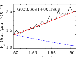
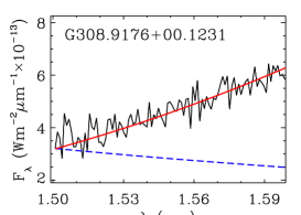
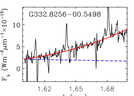
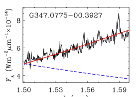
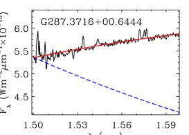
Figure 1: The RMS sources of which we have obtained low resolution NIR spectra as part of the follow-up program of observations for the RMS survey. The dashed line represents the Rayleigh-Jeans tail of a hot star ($F_{\lambda}\propto\lambda^{-4}$). The solid line is this tail reddened to fit the slope of the $H$-band spectra.

Table 2: The extinction (Cols 2 & 3) towards each object (Col. 1). The $A_{V}$ values are determined from the best-fitting $A_{K}$ values and the relationship between optical and NIR extinction from Cardelli et al. (1989). In addition, we present the $K$-band continuum flux density of each object, based on its $K$-band magnitude (Col. 4), and the estimated flux density at the peak of the CO $\mathrm{1^{st}}$ overtone bandhead (Col. 5). Finally, we de-redden the CO bandhead flux (Col. 6) and compare it to the flux of the best-fitting model (Col. 7). The uncertainty in the extinction values are estimated from assessing the fit to the continuum with $\chi^{2}$ (where the fitting range was specified to avoid lines and artefacts in the spectra). The uncertainty in the extinction is then used to determine the error in the flux.

Object	$A_{V}$	$A_{K}$	$\mathrm{F_{cont}}$	$\mathrm{F_{CO}}$(observed)	$\mathrm{F_{CO}}$(de-reddened)	$\mathrm{F_{CO}(model)}$
			$\mathrm{Wm^{-2}\mu m^{-1}}$	$\mathrm{Wm^{-2}\mu m^{-1}}$	$\mathrm{Wm^{-2}\mu m^{-1}}$	$\mathrm{Wm^{-2}\mu m^{-1}}$
IRAS 08576$-$4334	12†	1.4	5.8$\mathrm{\times 10^{-14}}$	4.4$\mathrm{\times 10^{-14}}$	1.6$\mathrm{\times 10^{-13}}$	2.8$\mathrm{\times 10^{-13}}$
G287.3716+00.6444	12	1.3$\pm$0.1	3.3$\mathrm{\times 10^{-13}}$	2.6$\mathrm{\times 10^{-14}}$	8.6$\pm$0.8$\mathrm{\times 10^{-14}}$	see Section 4.3
M8 E	25‡	2.8	5.8$\mathrm{\times 10^{-12}}$	8.1$\mathrm{\times 10^{-13}}$	1.1$\mathrm{\times 10^{-11}}$	6.2$\mathrm{\times 10^{-12}}$
G308.9176+00.1231	32	3.6$\mathrm{{}_{-0.5}^{+0.4}}$	9.1$\mathrm{\times 10^{-13}}$	7.3$\mathrm{\times 10^{-14}}$	2.0$\mathrm{{}_{-0.7}^{+0.9}}$$\mathrm{\times 10^{-12}}$	3.0$\mathrm{\times 10^{-12}}$
G033.3891+00.1989	22	2.5$\pm$0.3	4.4$\mathrm{\times 10^{-13}}$	5.2$\mathrm{\times 10^{-14}}$	5.2$\mathrm{{}_{-1.3}^{+1.6}}$$\mathrm{\times 10^{-13}}$	3.7$\mathrm{\times 10^{-13}}$
G332.8256$-$00.5498	70	2.4$\pm$0.3	9.1$\mathrm{\times 10^{-14}}$	1.9$\mathrm{\times 10^{-14}}$	1.7$\mathrm{{}_{-0.4}^{+0.6}}$$\mathrm{\times 10^{-13}}$	3.6$\mathrm{\times 10^{-13}}$
G347.0775$-$00.3927	23	2.6$\pm$0.3	1.3$\mathrm{\times 10^{-13}}$	1.3$\mathrm{\times 10^{-14}}$	1.4$\mathrm{{}_{-0.3}^{+0.5}}$$\mathrm{\times 10^{-13}}$	5.0$\mathrm{\times 10^{-14}}$

$\dagger$: Bik et al. (2006), ${\ddagger}$: Porter et al. (1998)

3 Results

3.1 The spectra

Continuum normalised spectra of the MYSO sample at $\mathrm{2.3\mu}$m are presented in Fig. 2. The objects exhibit a range of CO bandhead profiles. Some display a clear blue ‘shoulder’ at the bandhead (e.g. G332.8256$-$00.5498), while others exhibit a relatively sharp rise from the blue continuum to the bandhead (e.g. IRAS 08576$-$4334). The peak fluxes for the RMS objects are of order 10 per cent the continuum, much less than that of IRAS 08576$-$4334 ($\mathrm{\sim 80percent}$). Bandhead profiles with a prominent blue shoulder are indicative of emission from a rotating disc (e.g. Najita et al., 1996). None the less, the profiles with sharper edges to the bandhead can also be fit with disc models (see Bik & Thi, 2004), provided the disc is large or the inclination is low, thereby minimising the rotational broadening of the bandhead.

We used a simple model to first fit the bandhead profiles. We then compared the predicted spectroastrometric signatures of the best-fitting models with the data.

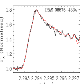
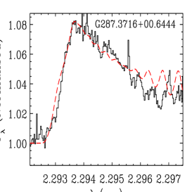
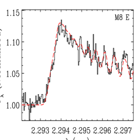
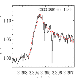
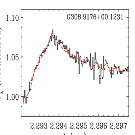
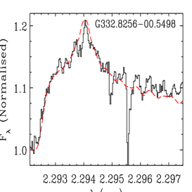
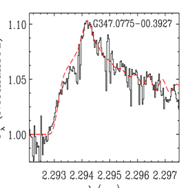
Figure 2: The spectra of the sample around the CO $\mathrm{1^{st}}$ overtone bandhead. The spectra have been divided by standard spectra, normalised, and re-binned by a factor of 3. The dashed line represents the best-fitting model, which is described in Section 3.2. The absorption features present in the spectra of G033.3891+00.1989 and G332.8256-00.5498 are residual telluric effects.

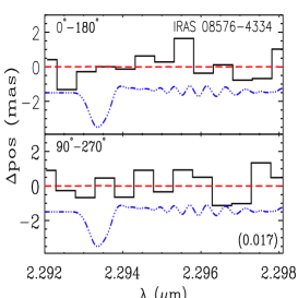
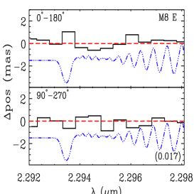
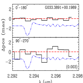
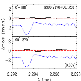
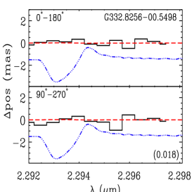
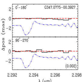
Figure 3: The spectroastrometric signatures of the sample over the CO $\mathrm{1^{st}}$ overtone bandhead emission, shown normalised to the continuum position. The data, the solid line, have been re-binned with a bin size of 65 $\mathrm{km\,s^{-1}}$ (approximately 11 times the resolution element). We also present the predicted signatures of the best-fitting model (see Section 3.3) for each object, bar G287.3716+00.6444 (see Section 4.3), to illustrate the signature of a rotating disc. The model signature is shown twice (at the un-binned spectral resolution): 1. with its predicted amplitude (dashed line), and 2. with an amplitude of 2 mas in the negative direction to enhance its visibility (offset dot-dashed line). The maximum predicted signature is presented in the lower right corner of each plot (in mas).

3.2 The model

The model of CO $\mathrm{1^{st}}$ overtone bandhead emission is based on Kraus et al. (2000). Initially, a simple, geometrically flat disc is constructed, within which the excitation temperature and surface number density decrease with increasing radius. The decrease in temperature and surface number density are treated as power laws. The temperature decreases with $R\mathrm{{}^{-0.75}}$ and the surface number density falls off with $R\mathrm{{}^{-1.5}}$, in line with standard accretion disc theory (Pringle, 1981), and following Kraus et al. (2000), who also modelled CO emission from a circumstellar disc. As the disc model is very simple and does not incorporate accretion the temperature of the disc is determined as follows: $T(R)=T_{\rm{eff}}\times(\frac{R}{R_{\star}})^{-0.75}$, where $T_{\rm{eff}}$ is set based on the luminosity of the star (assuming it to be on the main sequence). The disc is split into radial and azimuthal cells. If the temperature in a cell is greater than 5000 K (the assumed destruction temperature of CO), the flux from the cell is set to zero. If the outer radius of the disc is such that the outer cell temperatures are less than 1000 K the disc is shrunk until the temperature at the edge is 1000 K. Therefore, while the radii were varied during the fitting process, they are tied to the temperature structure of the disc. The CO emission of each cell is calculated according to the methodology of Kraus et al. (2000), which is briefly described in the following.

The population of the CO rotational levels (up to J=100) for the 2-0 vibrational transition in each cell is determined assuming local thermodynamic equilibrium. Then, the absorption coefficient is determined from the populations of the possible energy levels, and the transition probabilities of the respective lines. Assuming the absorption coefficient is constant along the line of sight, the optical depth is given by the product of the absorption coefficient per CO molecule and the CO column density. The column density is given by the surface number density, as we use a thin disc. The Dunham coefficients required to calculate the CO energy levels were taken from Farrenq et al. (1991), and the Einstein coefficients of each ro-vibrational transition were taken from Chandra et al. (1996). The intrinsic line profile is assumed to be Gaussian, with the line-width being a free parameter. Once the individual cell spectra are calculated, they are summed to create the total spectrum. This is then convolved with a Gaussian profile to match the spectral resolution of the observations.

To determine the best-fitting model, the downhill simplex algorithm was used. This algorithm is supplied with the Interactive Data Language distribution (IDL), and is based on the amoeba routine. The free parameters are: the inner and outer radius of the disc, the inclination of the disc, the surface number density at the inner edge of the disc and the line width within the disc. Once the best-fitting parameters have been determined the spectroastrometric signature of the best-fitting model is predicted. This is done by mapping the flux from each cell onto an array with orthogonal spatial and dispersion axes that represents a long-slit spectrum. The array is then convolved with a Gaussian profile in the spatial direction, to represent the seeing conditions. The synthetic signature is then generated by fitting a Gaussian profile to the spatial distribution at each dispersion pixel.

The stellar mass is not a free parameter and is set to that listed in Table 1, which is generally determined from the luminosity of the source and main sequence relationships (Martins et al., 2005). However, the luminosities of IRAS 08576$-$4334 and M8E are not known. Therefore, the mass of IRAS 08576$-$4334 was determined from its position in the $K$ vs $J-K$ diagram of Bik et al. (2006). We revise the distance to IRAS 08576$-$4334, and find it is still located in the mid- to early B area of the $K$ vs $J-K$ diagram, and hence assume it has the mass of a B3 type star. The mass of M8E was taken from Linz et al. (2009), and is the mass of the best-fitting model from the grid of models by Robitaille et al. (2007).

Using the luminosity of a MYSO to determine its mass is subject to some uncertainty as the observed luminosity may be due in part to accretion, resulting in an overestimate of the stellar mass. To evaluate the possible effect this may have, we consulted the models of accreting, massive protostars presented by Hosokawa & Omukai (2009). During the early adiabatic accretion phase, the accretion luminosity of a massive protostar is greater than its intrinsic luminosity. However, by the time a massive protostar enters its main sequence accretion phase the intrinsic luminosity is greater than the accretion luminosity. While the resultant total luminosity is slightly greater than the zero age main sequence luminosity the two are not different by an order of magnitude. Given the high luminosity of the sample objects, it is likely they are in the Kelvin-Helmholtz contraction or main sequence accretion phases. Therefore, it is unlikely we significantly overestimate their luminosity. Furthermore, given that the objects are most likely in their main sequence accretion phase, the main sequence relationship between mass and luminosity should be applicable. Therefore, it is surmised that using main sequence relationships is sufficient for the purposes of this paper.

3.3 Model fits and results

Over the wavelength range at our disposal few individual ro-vibrational lines are visible. The fitting process is therefore dominated by the shape of the CO bandhead peak and shoulder. The appearance of the shoulder is set by the rotational profile of the individual lines, and is thus dependent on the inclination and the inner and outer disc radii (as the stellar mass is not varied). However, the temperature of the disc is also a function of distance from the central star. In general few individual lines are evident, indicative of relatively high temperatures – and/or high rotational broadening. As a result, the inner disc radii are generally small, of the order 0.1 au. Changing the outer radii has little effect on the quality of the fit as the surface number density, and thus flux, fall off steeply. As a consequence, it is the inclination that dominates the fit to the bandhead profile. The object with the most prominent blue shoulder is fit with the largest inclination (G332.8256$-$00.5498: $\mathrm{\sim 42^{\circ}}$), while the objects with the steepest slopes from the blue continuum to the bandhead peak (IRAS 08576$-$4334 and M8E) are fit with the lowest inclinations ($\mathrm{\sim 18^{\circ}}$ & $\mathrm{16^{\circ}}$).

The best fit parameters are presented in Table 3, and the resultant bandhead profiles are plotted with the data in Fig. 2. As can be seen from the reduced $\mathrm{\chi^{2}}$ values (the mean is 1.68) the model of CO emission originating from a circumstellar disc generally provides a good fit to the data. The sole exception to this is G287.3716+00.6444, which is discussed in more detail in Section 4.3.

We compare the predicted bandhead fluxes with the un-reddened observed fluxes as a consistency check. As mentioned in Section 2.3, these un-reddened fluxes are inevitably subject to considerable uncertainties, yet still serve as an important validity test. We list both model and source fluxes in Table 2. These are similar to within a factor of 2–3, and generally consistent within the uncertainty from the extinction estimate (neglecting the addition error due to uncertainties in the kinematic distances). Therefore, the observed and model fluxes are essentially consistent. This provides a further confirmation that disc models provide a good fit to the data.

Table 3: The parameters of the best-fitting models. The mass is determined from the luminosity presented in Table 1. The uncertainties in $i$, $NCO_{\rm{in}}$ and $\Delta v$ are determined by holding all other parameters constant and determining the change required to increase the reduced $\chi^{2}$ by 1.0.

Name	Mass	Inclination	${R_{\rm{in}}^{{\ddagger}}}$	${R_{\rm{out}}^{\ast}}$	$NCO_{\rm{in}}$	$\mathrm{\Delta}v$	$\chi^{2}$
	($\mathrm{M_{\odot}}$)	(∘)	(au)	(au)	($\mathrm{cm^{-2}}$)	($\mathrm{km\,s^{-1}}$)
IRAS 08576$-$4334	6.1	17.8$\mathrm{{}_{-0.4}^{+0.8}}$	0.09	0.78	7.9$\mathrm{{}_{-1.7}^{+1.3}}$$\mathrm{\times 10^{21}}$	20.0$\mathrm{{}_{-3.1}^{+3.1}}$	2.18
G287.3716+00.6444	See Section 4.3
M8 E	13.5	15.8$\mathrm{{}_{-2.8}^{+2.0}}$	0.31	2.61	1.1$\mathrm{{}_{-1.1}^{+7.9}}$$\mathrm{\times 10^{23}}$	7.6$\mathrm{{}_{-2.8}^{+2.0}}$	1.38
G033.3891+00.1989	11.8	18.0$\mathrm{{}_{-3.7}^{+2.8}}$	0.24	2.05	9.4$\mathrm{{}_{-6.6}^{+7.6}}$$\mathrm{\times 10^{21}}$	19.9$\mathrm{{}_{-16.1}^{+36.4}}$	1.95
G308.9176+00.1231	42.6	29.0$\mathrm{{}_{-3.9}^{+5.4}}$	0.94	8.00	4.9$\mathrm{{}_{-3.3}^{+12.9}}$$\mathrm{\times 10^{22}}$	13.6$\mathrm{{}_{-8.6}^{+15.0}}$	1.14
G332.8256$-$00.5498	24.5	42.3$\mathrm{{}_{-11.7}^{+4.4}}$	0.59	5.08	2.2$\mathrm{{}_{-{\dagger}}^{+5.7}}$$\mathrm{\times 10^{21}}$	18.6$\mathrm{{}_{-17.6}^{+35.4}}$	2.79
G347.0775$-$00.3927	17.7	30.6$\mathrm{{}_{-14.3}^{+15.0}}$	0.45	3.81	1.7$\mathrm{{}_{-{\dagger}}^{+7.4}}$$\mathrm{\times 10^{22}}$	19.9$\mathrm{{}_{-18.9}^{+86.2}}$	0.62

${\ddagger}$: No uncertainties are presented as these inner radii are the inner radii of the region where CO emission is possible, i.e. $T\mathrm{<5000K}$. Therefore, decreasing the inner radii did not affect the quality of the fits.
$\ast$: No uncertainties are presented as these outer radii are the outer radii of the region where CO emission is possible, i.e. $T\mathrm{>1000K}$. Therefore, increasing the outer radii did not affect the quality of the fits.
${\dagger}$: $\chi^{2}$ flat down to $\mathrm{10^{18}cm^{-2}}$, the minimum surface number density considered. Therefore, no error is presented here.

3.4 Spectroastrometric signatures

The spectroastrometric signatures associated with the spectra presented in Fig. 2 are displayed in Fig. 3. The spectroastrometric data have been re-binned by a factor of $\mathrm{\sim}$11 times the resolution element. This rebinning factor was chosen as it was the maximum bin size that could still resolve the expected spectroastrometric signatures across the bandhead. The resulting average positional precision is approximately 0.4 mas. In principle, this means we are probing au size scales at the kpc distances of the sample. Here, we compare the spectroastrometric data to the best-fitting models to determine whether these data can be used to further probe the circumstellar environments of the sample.

The spectroastrometric signatures associated with the best-fitting models are also presented in Fig. 3. The predicted signatures are generally small, and to illustrate their appearance, an enhanced spectrum is shown offset in each panel. The largest excursion occurs on the blue side of the bandhead, which is due to the asymmetry of the bandhead profile. Over the blue shoulder of the bandhead all the emission is blue-shifted. Therefore, at these wavelengths the side of the disc coming towards the observer is significantly brighter than the other side, which results in the prominent spectroastrometric signature at these wavelengths. Conversely, red-wards of the bandhead peak the receding side of the disc is brightest, resulting in a positional excursion in the opposite direction. However, at these wavelengths red-shifted emission from the peak of the bandhead is mixed with blue-shifted emission of ro-vibration lines at longer wavelengths. As a consequence, the spectroastrometric signature is smaller to the red of the bandhead peak than on the blue side. Over individual, resolved ro-vibrational lines the two sides of the disc are almost equally bright, and thus the excursions at positive and negative velocities are nearly symmetrical, resulting in the classic ‘S’ shaped signature of a disc (Pontoppidan et al., 2008; van der Plas et al., 2009, Wheelwright et al. in prep.). As the individual ro-vibrational lines are located close together the adjacent positional signatures result in an oscillating signature.

The largest predicted excursions are of the order 0.01 mas, which is much smaller than the precision of the spectroastrometric data. The small scale of the spectroastrometric signatures is largely due to the large distances to the science objects, coupled with relatively weak CO emission, which is typically 10 per cent of the continuum flux. The largest predicted signatures are those of IRAS 08576$-$4334 and M8E (both 0.017 mas), due to their proximity. Even with a positional precision of 0.15 mas, the best in the sample, such excursions would not be detected.

While the spectroastrometric data do not provide useful constraints to the model fitting process, they are entirely consistent with the best-fitting models of emission originating in circumstellar discs. Moreover, the data do provide additional constraints on the source of the emission. We note that the spectroastrometric signature of IRAS 08576$-$4334 exhibits no detectable excursion with a precision of approximately 0.7 mas. This is contrary to the finding of Grave & Kumar (2007), who report an excursion of approximately 18 mas, corresponding to a minimum size of 40 au at 2.17 kpc, and likely several times this. We suggest that the feature in their data is an instrumental artefact, which is not present in our data as our practice of subtracting anti-parallel position spectra eliminates artefacts (the data of Grave & Kumar (2007) were obtained using a constant PA.)

4 Discussion

4.1 A discussion on the best-fitting parameters

The best-fitting inner disc radii are typically of the order 0.1 au, and the best-fitting outer disc radii are generally 1–5 au. These values are consistent with those of Bik & Thi (2004), and indicate that the CO emission arises from small scale circumstellar discs. At such small distances from the central star, CO molecules should be disassociated by ultraviolet photons. However, the best-fitting number surface densities are sufficient for the CO molecules to self-shield, as found by Bik & Thi (2004). We note that the simplistic treatment of the temperature gradient within the disc allows CO to be excited within 1 au of the central star. However, a full treatment of viscous heating in such a disc keeps the mid-plane temperature above $\mathrm{\sim}$5000 K out to approximately 1 au (Vaidya et al., 2009). This would have the effect of moving the inner radius of the CO emitting region further from the central star. The difference between the best-fitting inner radii and the radius at which the mid-plane temperature of a massive accretion disc drops below 5000K is of the order a few, and thus is unlikely to significantly affect the best-fitting properties. In addition, the viscous heating is dependent upon the accretion rate, which is uncertain and thus incorporating viscous heating in the model would introduce an additional unknown. Therefore, we judge the simplistic temperature gradient to be sufficient for the purposes of this paper.

In the model the excitation temperature in the disc varies as a function of radius. If the disc is sufficiently large the outer temperature falls below 1000 K and the outer cells contribute no flux to the total spectrum. In this situation increasing the outer radius will not affect the resultant $\chi^{2}$, as the output spectrum will not be changed. However, the physical disc may well be much larger than the CO emitting region, which constitutes the warmer and denser part of the disc. In this respect the outer regions of the CO emitting region are consistent with the models of Vaidya et al. (2009), who show that accretion discs around massive protostars may well be stable out to approximately 80 au. The dust sublimation radii associated with MYSOs are typically greater than 10 au (de Wit et al., 2007; Vaidya et al., 2009). Therefore, the CO emission of the best-fitting models originates from within the dust sublimation radius, and thus offers a unique tracer of gas prior to its accretion onto the central star.

The inner radii set the initial excitation temperature, which is a function of the distance from the central star. As a result, changing the inner radius effects both the temperature in the disc and the rotational broadening of the bandhead. To consistently determine the temperature structure of the disc, and thus more stringent constraints, a detailed radiative transfer model of the disc is required. However, even if the gas disc were modelled in detail, the properties of the central star are essentially unknown. For example the star may swell to several times its main sequence size as a consequence of high accretion rates (Hosokawa & Omukai, 2009), which will reduce its effective temperature. Therefore, even a sophisticated disc model wold be subject to several unknowns.

The best-fitting line-widths are generally greater than the value of $\mathrm{\sim 4\,km\,s^{-1}}$ determined by Berthoud et al. (2007), who fit the CO $\mathrm{1^{st}}$ overtone emission of the Be star 51 Oph with a circumstellar disc model. The line widths are also approximately ten times the thermal broadening due to motion of the CO molecules. Therefore, the dominant contribution must be due to turbulence. However, we do not consider shear broadening in the model. If this were taken into account, the turbulent velocity may well be less than the best-fitting values presented in Table 3. The properties of accretion discs around MYSOs has only recently begun to be examined in detail (Vaidya et al., 2009), and incorporating vertical disc structure to the disc model (which is required to assess shear broadening Horne & Marsh, 1986; Hummel & Vrancken, 2000) is beyond the scope of this paper. Therefore, we neglect shear velocity. However, it is important to note that neglecting vertical structure may artificially limit the extent of the CO emitting region. In a disc with a vertical extent the upper regions of the disc may be hot enough to excite CO emission at radii where the mid-plane temperature has dropped below the required $\mathrm{\sim 2000~{}K}$. Therefore, incorporating vertical structure in the model may allow CO emission from a wider range of radii than the thin disc model. This would have the effect of increasing the resulting spectro-astrometric signatures, and thus the predictions presented here may be lower limits.

4.2 Comparisons with previous work

Little is known about the circumstellar environments of the RMS objects. In particular, there are no previous high resolution studies with which to compare the best-fitting model parameters. However, the two non-RMS objects in the sample, M8 E and IRAS 08576$-$4334 have been both been studied previously. Here, we assess whether the best-fitting models for these objects are consistent with other observations.

Bik & Thi (2004) determine the inclination of IRAS 08576$-$4334 to be $\mathrm{27^{{\circ}+2}_{-14}}$ based on fitting the CO $\mathrm{1^{st}}$ overtone bandhead. The best-fitting value of $\mathrm{\sim 18^{\circ}}$ determined here is thus consistent with the previous value. This might be expected as we apply the same methodology, none the less, this provides an important check that the results are consistent with previous work. Turning to M8E, Simon et al. (1985) postulate that this object possesses an edge on disc; contrary to our best-fitting inclination of $\mathrm{\sim 16^{\circ}}$. However, Linz et al. (2009) find an inclination $\mathrm{<30^{\circ}}$ is required to fit the SED of M8E. These authors suggest that the interpretation of the lunar occultation data of Simon et al. (1985) is complicated by the presence of scattered light and outflow cavities. Given that the conclusion of Linz et al. (2009) is based on the SED of M8 E from the visible to mid infrared, in addition to the grid of models of Robitaille et al. (2007), we suggest the inclination determined by Linz et al. (2009) is currently the best estimate, which is in agreement with the best-fitting value. Therefore, we conclude that the best-fitting models are consistent with results in the literature, although only a few are available, indicating that the best-fitting model parameters are representative of the circumstellar environments of the sample.

4.3 G287.3716+00.6444

In all but one case, the disc model not only provided a good fit to the data (as measured with $\chi^{2}$), but was also consistent with the observed flux densities, and where they existed, previous observations. Therefore, it would appear that small scale discs are present around the majority of the sample. However, it was not possible to fit the CO $\mathrm{1^{st}}$ overtone bandhead of G287.3716+00.6444 with the circumstellar disc model used to fit the other profiles. As shown in Fig. 2 the disc model could not fit observed the bandhead shoulder, nor the slope red-wards of the peak. Furthermore, the bandhead could not be fit with emission from an isothermal, non-rotating body of CO. Therefore, we are led to consider alternative scenarios to explain the emission and its profile.

Besides hot, dense discs there are other viable sources of CO $\mathrm{1^{st}}$ overtone bandhead emission. One such scenario is a dense, neutral wind. Chandler et al. (1995) were able to fit the CO $\mathrm{1^{st}}$ overtone bandheads of several YSOs with models of neutral winds, but note that the mass loss rates required were relatively high, up to $\mathrm{10^{-6}\,M_{\odot}yr^{-1}}$. Chandler et al. (1995) consider it unlikely CO $\mathrm{1^{st}}$ overtone emission originates in a wind as such mass loss rates are much higher than observed for solar mass YSOs. However, the winds of MYSOs may well lead to mass loss rates of $\mathrm{10^{-6}\,M_{\odot}yr^{-1}}$ (Drew et al., 1993). Consequently, CO $\mathrm{1^{st}}$ overtone emission from a dense wind should perhaps be re-considered in this case. Alternatively, Scoville et al. (1983) propose that the CO $\mathrm{1^{st}}$ overtone bandhead emission of the Becklin-Neugebauer object is created in shocks (as the observed velocity dispersion and estimated emitting area are both small).

We note that Blum et al. (2004) also report that the CO $\mathrm{1^{st}}$ overtone bandhead of one of their sample (of four YSOs) was difficult to fit with a model of CO emission from a circumstellar disc. Following the example of Kraus et al. (2000), they suggest that this may be due to the circumstellar disc exhibiting an outer bulge, which shields the inner regions of the disc. The effect of this would be to limit the visible CO emitting region to low velocity regions, resulting in a narrow profile. In this case, however, it is not the width of the profile we cannot fit, but rather the slope of the profile red-wards of the bandhead peak. Most formation scenarios, such as winds and discs, result in excess blue-shifted emission, therefore this bandhead profile is difficult to explain.

It is conceivable that the emission from several, discrete regions in a shock, will have different excitation temperatures, and when superimposed, will result in a different slope to the bandhead than the disc model. If such shocks exist, the shocked region must be located close to the central star, within a few au, as we do not see a positional excursion in the spectroastrometric data. However, it is difficult to envisage a scenario in which the shock emission is predominately red-shifted. As an alternative it may be that the emission does originate in a disc, but the receding part of the disc is significantly brighter than the approaching side, similar to the V/R variations exhibited by Be stars (e.g. Hanuschik et al., 1995). Regardless, it is apparent that while the majority of MYSO CO bandheads are well fit by models of circumstellar discs, the circumstellar environments of MYSOs are not yet completely understood.

5 Conclusions

In this paper we present high resolution near infrared spectroastrometry around 2.3$\mathrm{\mu m}$ of a sample of young stellar objects, most of which are drawn from the RMS survey. The RMS constitutes the largest catalogue of massive young stellar objects to date, and thus provides a unique sample to study massive star formation. We model the CO $\mathrm{1^{st}}$ overtone bandhead emission detected with a simple model of a circumstellar disc in Keplerian rotation. In addition, the sub milli-arcsecond precision spectroastrometric data are compared to the spatial signatures of the best-fitting models.

The observed bandhead profiles are, on the whole, well fit by models of the emission originating in circumstellar discs. This concurs with the generally accepted view that this emission arises in small scale accretion discs. The observed bandhead of one object cannot be fit with a circumstellar disc model. This could be due to the emission emanating from an asymmetric disc or shock. This highlights that the circumstellar environments of massive young stellar objects are still not completely understood.

No spatial signatures of discs are revealed in the spectroastrometric data, which have a precision of approximately 0.4 mas. This is entirely consistent with the sizes of the best-fitting models. Due to the small sizes of the discs, the large distances to them and the decrease in brightness with radius the predicted signatures are of the order of $\mathrm{0.01mas}$. This is well below the current detection limit. However, the predicted signatures could perhaps be revealed by differential phase observations with AMBER. Currently, MYSOs are below the sensitivity limit of AMBER, but PRIMA should allow us to observe such objects and probe the spatial distribution of the CO emission at an even higher precision.

To summarise, in general the model of emission from a circumstellar disc provides a good fit to the observed bandheads, and is consistent with the observed flux densities. This indicates that the majority of MYSOs with CO $\mathrm{1^{st}}$ overtone emission possess small-scale, circumstellar discs. In turn, this provides further evidence that massive stars form via disc accretion, as suggested by the simulations of Krumholz et al. (2009).

References

- Bailey (1998) Bailey J. A., 1998, Proc. SPIE, 3555, 932
- Baker & Menzel (1938) Baker J. G., Menzel D. H., 1938, ApJ, 88, 52
- Bally & Zinnecker (2005) Bally J., Zinnecker H., 2005, AJ, 129, 2281
- Beltrán et al. (2005) Beltrán M. T., Cesaroni R., Neri R., Codella C., Furuya R. S., Testi L., Olmi L., 2005, A&A, 435, 901
- Berthoud et al. (2007) Berthoud M. G., Keller L. D., Herter T. L., Richter M. J., Whelan D. G., 2007, ApJ, 660, 461
- Bik et al. (2006) Bik A., Kaper L., Waters L. B. F. M., 2006, A&A, 455, 561
- Bik & Thi (2004) Bik A., Thi W. F., 2004, A&A, 427, L13
- Blum et al. (2004) Blum R. D., Barbosa C. L., Damineli A., Conti P. S., Ridgway S., 2004, ApJ, 617, 1167
- Bonnell et al. (1998) Bonnell I. A., Bate M. R., Zinnecker H., 1998, MNRAS, 298, 93
- Brand & Blitz (1993) Brand J., Blitz L., 1993, A&A, 275, 67
- Bronfman et al. (1996) Bronfman L., Nyman L., May J., 1996, A&AS, 115, 81
- Cardelli et al. (1989) Cardelli J. A., Clayton G. C., Mathis J. S., 1989, ApJ, 345, 245
- Carr (1989) Carr J. S., 1989, ApJ, 345, 522
- Cesaroni et al. (2007) Cesaroni R., Galli D., Lodato G., Walmsley C. M., Zhang Q., 2007, in B. Reipurth, D. Jewitt, & K. Keil ed., Protostars and Planets. Univ. Arizona Press, Tucson, 197
- Chan et al. (1996) Chan S. J., Henning T., Schreyer K., 1996, A&AS, 115, 285
- Chandler et al. (1995) Chandler C. J., Carlstrom J. E., Scoville N. Z., 1995, ApJ, 446, 793
- Chandra et al. (1996) Chandra S., Maheshwari V. U., Sharma A. K., 1996, A&AS, 117, 557
- Chini & Neckel (1981) Chini R., Neckel T., 1981, A&A, 102, 171
- Clarke et al. (2006) Clarke A. J., Lumsden S. L., Oudmaijer R. D., Busfield A. L., Hoare M. G., Moore T. J. T., Sheret T. L., Urquhart J. S., 2006, A&A, 457, 183
- Cutri et al. (2003) Cutri R. M. et al., 2003, 2MASS All Sky Catalog of Point Sources. Astron. Soc. Pac., San Fransisco
- Davies et al. (2010) Davies B., Lumsden S. L., Hoare M. G., Oudmaijer R. D., de Wit W.-J., 2010, MNRAS, 402, 1504
- Davis et al. (2004) Davis C. J., Varricatt W. P., Todd S. P., Ramsay Howat S. K., 2004, A&A, 425, 981
- de Wit et al. (2009) de Wit W. J., Hoare M. G., Oudmaijer R. D., Lumsden S. L., 2009, ArXiv e-prints
- de Wit et al. (2007) de Wit W. J., Hoare M. G., Oudmaijer R. D., Mottram J. C., 2007, ApJL, 671, L169
- Drew et al. (1993) Drew J. E., Bunn J. C., Hoare M. G., 1993, MNRAS, 265, 12
- Egan et al. (2003) Egan M. P., Price S. D., Kraemer K. E., 2003, Bull. Am. Astron. Soc., 35, 1301
- Farrenq et al. (1991) Farrenq R., Guelachvili G., Sauval A. J., Grevesse N., Farmer C. B., 1991, JMoSp, 149, 375
- Grave & Kumar (2007) Grave J. M. C., Kumar M. S. N., 2007, A&A, 462, L37
- Hanuschik et al. (1995) Hanuschik R. W., Hummel W., Dietle O., Sutorius E., 1995, A&A, 300, 163
- Harmanec (1988) Harmanec P., 1988, Bull. Astron. Inst. Czechoslovakia, 39, 329
- Hinkle et al. (1995) Hinkle K., Wallace L., Livingston W., 1995, PASP, 107, 1042
- Hinkle et al. (2000) Hinkle K. H., Joyce R. R., Sharp N., Valenti J. A., 2000, SPIE Conf. Ser., 4008, 720
- Horne & Marsh (1986) Horne K., Marsh T. R., 1986, MNRAS, 218, 761
- Hosokawa & Omukai (2009) Hosokawa T., Omukai K., 2009, ApJ, 691, 823
- Hummel & Vrancken (2000) Hummel W., Vrancken M., 2000, A&A, 359, 1075
- Kaeufl et al. (2004) Kaeufl H. et al., 2004, SPIE Conf. Ser., 5492, 1218
- Kahn (1974) Kahn F. D., 1974, A&A, 37, 149
- Kraus et al. (2000) Kraus M., Krügel E., Thum C., Geballe T. R., 2000, A&A, 362, 158
- Krumholz et al. (2009) Krumholz M. R., Klein R. I., McKee C. F., Offner S. S. R., Cunningham A. J., 2009, Sci, 323, 754
- Landini et al. (1984) Landini M., Natta A., Salinari P., Oliva E., Moorwood A. F. M., 1984, A&A, 134, 284
- Larson & Starrfield (1971) Larson R. B., Starrfield S., 1971, A&A, 13, 190
- Linz et al. (2009) Linz H. et al., 2009, A&A, 505, 655
- Lumsden et al. (2002) Lumsden S. L., Hoare M. G., Oudmaijer R. D., Richards D., 2002, MNRAS, 336, 621
- Lumsden & Puxley (1996) Lumsden S. L., Puxley P. J., 1996, MNRAS, 281, 493
- Martins et al. (2005) Martins F., Schaerer D., Hillier D. J., 2005, A&A, 436, 1049
- Molinari et al. (1996) Molinari S., Brand J., Cesaroni R., Palla F., 1996, A&A, 308, 573
- Moore et al. (2005) Moore T. J. T., Lumsden S. L., Ridge N. A., Puxley P. J., 2005, MNRAS, 359, 589
- Mottram et al. (2010) Mottram J. C., Hoare M. G., Lumsden S. L., Oudmaijer R. D., Urquhart J. S., Meade M. R., Moore T. J. T., Stead J. J., 2010, A&A, 510, A89
- Mottram et al. (2007) Mottram J. C., Hoare M. G., Lumsden S. L., Oudmaijer R. D., Urquhart J. S., Sheret T. L., Clarke A. J., Allsopp J., 2007, A&A, 476, 1019
- Najita et al. (1996) Najita J., Carr J. S., Glassgold A. E., Shu F. H., Tokunaga A. T., 1996, ApJ, 462, 919
- Okamoto et al. (2009) Okamoto Y. K. et al., 2009, ApJ, 706, 665
- Oudmaijer et al. (2008) Oudmaijer R., Parr A., Baines D., Porter J., 2008, A&A, 489, 627
- Patel et al. (2005) Patel N. A. et al., 2005, Nat, 437, 109
- Pontoppidan et al. (2008) Pontoppidan K. M., Blake G. A., van Dishoeck E. F., Smette A., Ireland M. J., Brown J., 2008, ApJ, 684, 1323
- Porter et al. (1998) Porter J. M., Drew J. E., Lumsden S. L., 1998, A&A, 332, 999
- Price et al. (2001) Price S. D., Egan M. P., Carey S. J., Mizuno D. R., Kuchar T. A., 2001, AJ, 121, 2819
- Pringle (1981) Pringle J. E., 1981, ARA&A, 19, 137
- Robitaille et al. (2007) Robitaille T. P., Whitney B. A., Indebetouw R., Wood K., 2007, ApJS, 169, 328
- Scoville et al. (1983) Scoville N., Kleinmann S. G., Hall D. N. B., Ridgway S. T., 1983, ApJ, 275, 201
- Shepherd et al. (2001) Shepherd D. S., Claussen M. J., Kurtz S. E., 2001, Sci, 292, 1513
- Shu et al. (1987) Shu F. H., Adams F. C., Lizano S., 1987, ARA&A, 25, 23
- Simon et al. (1985) Simon M., Peterson D. M., Longmore A. J., Storey J. W. V., Tokunaga A. T., 1985, ApJ, 298, 328
- Sridharan et al. (2002) Sridharan T. K., Beuther H., Schilke P., Menten K. M., Wyrowski F., 2002, ApJ, 566, 931
- Stead & Hoare (2009) Stead J. J., Hoare M. G., 2009, MNRAS, 400, 731
- Storey & Hummer (1995) Storey P. J., Hummer D. G., 1995, MNRAS, 272, 41
- Takami et al. (2003) Takami M., Bailey J., Chrysostomou A., 2003, A&A, 397, 675
- Urquhart et al. (2007) Urquhart J. S., Busfield A. L., Hoare M. G., Lumsden S. L., Clarke A. J., Moore T. J. T., Mottram J. C., Oudmaijer R. D., 2007, A&A, 461, 11
- Urquhart et al. (2007) Urquhart J. S. et al., 2007, A&A, 474, 891
- Urquhart et al. (2008) Urquhart J. S. et al., 2008, A&A, 487, 253
- Urquhart et al. (2008) Urquhart J. S., Hoare M. G., Lumsden S. L., Oudmaijer R. D., Moore T. J. T., 2008, ASP Conf. Ser., 387, 381
- Urquhart et al. (2009) Urquhart J. S. et al., 2009, A&A, 501, 539
- Vaidya et al. (2009) Vaidya B., Fendt C., Beuther H., 2009, ApJ, 702, 567
- van der Plas et al. (2009) van der Plas G., van den Ancker M. E., Acke B., Carmona A., Dominik C., Fedele D., Waters L. B. F. M., 2009, A&A, 500, 1137
- Wheelwright et al. (2010) Wheelwright H. E., Oudmaijer R. D., Goodwin S. P., 2010, MNRAS, 401, 1199
- Wolfire & Cassinelli (1987) Wolfire M. G., Cassinelli J. P., 1987, ApJ, 319, 850
- Yorke & Sonnhalter (2002) Yorke H. W., Sonnhalter C., 2002, ApJ, 569, 846
- Zinnecker & Yorke (2007) Zinnecker H., Yorke H., 2007, ARA&A, 45, 481