Abstract

In this paper, we investigate the back-reaction of $U(1)$ gauge fields into a specific class of inflationary settings. To be more precise, we employ a Bianchi-I geometry (taken as an anisotropic perturbation of a flat FRW model) within two types of Born-Infeld theories. Firstly, we consider pure Born-Infeld electromagnetism. For either a constant or a $b(\phi)$ coupling, inflationary trajectories are modified but anisotropies increase; In particular, for the former coupling we find that a quadratic inflaton potential, within a constant ratio for the scalar and gauge energy densities, does not induce sufficient inflation, while in the latter the back-reaction in the cosmology determines (from the tensor-scalar ratio) a narrow range where inflation can occur. A Dirac-Born-Infeld framework is afterwards analysed in both non-relativistic and relativistic regimes. In the former, for different cases of the coupling (richer with respect to mere BI setups) between scalar and gauge sectors, we find that inflationary trajectories are modified, with anisotropy increasing or decreasing. In particular, a tachyonic solution is studied, allowing for a non standard ratio between scalar and gauge matter densities, enhancing sufficient inflation, but with the anisotropy increasing. For the relativistic limit, inflationary trajectories are also modified and anisotropies increase faster than in the non-relativistic limit. Finally we discuss how magnetic seed fields could evolve in these settings.

1 Introduction

Modern cosmology has entered a new phase of precision, unthinkable only two decades ago [1]. However a fundamental issue remains open; namely the origin of galactic and cosmological magnetic fields. Such fields have coherence length of the order $1$ Mpc, with a magnitude of around $10^{-7}G$ [2, 3]. The current explanation for the origin of such fields is that a small seed field emerged during primordial inflation, which was amplified at late times by the galactic dynamo mechanism [4, 5]; Cf. [6, 7, 8, 9, 10] and references therein for additional elements on cosmic magnetogenesis. As is well known from cosmological perturbation theory, the accelerated expansion stretches small scale physics to cosmological size, therefore it would appear natural to include a primordial magnetic field (e.g., a fluctuation) in models of early universe cosmology. A crucial feature in this setting is that a FRW cosmology with canonical fields is conformally invariant, therefore a mechanism to break the conformal invariance is necessary for magnetic fields to be present [11]. Proposals of solutions to this problem are discussed in [3, 5].

Additionally, dealing with a vector (gauge) field in cosmology may require some degree of anisotropy [14]. Therefore we must go beyond the simplest FRW models to understand the dynamics of the universe with a magnetic field. In this context, let us mention the various anomalies present in the CMB, such as the suppression and asymmetries of the power spectrum in different hemispheres, together with the presence of a preferred direction due to the alignment of lowest multipole moments [15, 16]. These anomalies can be interpreted as a sign that isotropic statistics are only a leading order approximation, and that these anomalous measurements are due to non-isotropic expansion. Hence, it is reasonable to investigate (inflationary) anisotropic space-times with a non-zero gauge field.

Model building with both magnetic seed fields and anisotropies has been explored in [17, 18, 19, 20, 21]. One potential pitfall present in those references was that the magnetic field energy density grows rapidly during an inflationary phase, and was thought to destroy the inflationary dynamics. As pointed out in [18], this claim was not based on concrete analysis and in fact was shown to be false. Inflation does occur in the presence of a gauge field and leads to weakly growing anisotropy - but is modified by the back-reaction on the inflaton [22, 23]. This was due to the gauge field acting as a source term in the Klein-Gordon equation, whilst remaining subdominant to the scalar energy density in the Hubble parameter. The overall net effect was to further suppress the amplitude of magnetic field production after inflation. The above analysis refers to (canonical) Einstein-scalar-Maxwell theory. However within the context of open string theory, the effective action is non-linear and we can ask how the above results are modified by such non-linearities.

Our purpose in this paper is to extend the discussion on gauge fields back-reacting on inflationary cosmologies (and how magnetic seed fields can emerge and evolve consequently) to a class of non-linear theories described by Born-Infeld (BI) type Lagrangians. Within string theory, we have a Lagrangian description of the low energy regime of a (Dirichlet) $Dp$-brane, which in a cosmological context gives rise to a class of theories known as Dirac-Born-Infeld (DBI) inflation. The inclusion of gauge fields in such models have been considered in [24, 25], but here we incorporate instead the ideas of anisotropic inflation and attempt to generalise the results. Moreover these papers assumed warped backgrounds which were asymptotically AdS, however more general classes of backgrounds are not asymptotically AdS which leads to non-trivial coupling between the gauge field and the dilaton. By assuming an extra condition, which we believe to be physically motivated, fixing the electromagnetic energy density in terms of the scalar energy density - we can consider more general configurations.

Our paper is presented as follows. In section 2 we consider a simple BI theory, which reduces to the Einstein-Maxwell theory in a specific limit. In subsection 2.1 we take the usual BI configuration and in subsection 2.2 we analyse the gauge and scalar sectors through a $b(\phi)$ coupling. In both cases, we investigate how the gauge field back-reaction affects the inflationary dynamics. In particular, we describe how inflation can be modified and whether the anisotropies will increase or not. In section 3 we employ a phenomenological model of DBI inflation using a generalised expression for the $D3$-brane action. We consider the back-reaction of the gauge field in several different regimes. In particular, the energy density can be constrained so that inflation is driven by the scalar sector. In subsection 3.1 we discuss the non-relativistic limit, together with a tachyon configuration followed by a $AdS_{5}$ solution. In subsection 3.2 we take the relativistic limit. In section 4 we conclude with a discussion of our results and suggestions for future work. In Appendix A we determine how magnetic seed fields can be generated and how DBI ingredients can contribute to the magneto cosmogenesis discussion.

2 Born-Infeld theory

In this section we consider the non-linear extension of the Einstein-Maxwell theory ($U(1)$ gauge field) to the Einstein-Born-Infeld theory. Such a theory automatically includes electro-magnetic duality, and a causal structure that implies that the electromagnetic field is everywhere finite. Other works detailing non-linear Lagrangian densities include [26, 27, 28, 29]. A similar framework plays an important role in the effective description of $D$-branes within string theory, and therefore serves as a toy model for a more detailed analysis of open string dynamics.

The matter Lagrangian for such a model can be written as follows

$$\mathcal{L}=-\frac{1}{2}\partial_{\mu}\phi\partial^{\mu}\phi-V(\phi)+\frac{1}{b}\left(1-\sqrt{1+\frac{b}{2}F_{\sigma\rho}F^{\sigma\rho}}\right),$$ (2.1)

where $b$ is the BI parameter. One can see that as $b\to 0$ the theory is reduced so that it includes the Maxwell form; However the non-linear nature of the Lagrangian means that we can think of $b$ as a deformation parameter which has mass dimension $M^{-4}$. Cosmologically therefore, we expect $b$ to deform the conformal nature of the gauge field term. We wish to study the implications of such a gauge field correction on the inflationary dynamics.

Using the residual gauge invariance, we consider solutions where $A_{0}=0$ and assume that the homogeneous vector potential $A$ is aligned (and fixed) along the $x$-direction. This breaks the (spatial) $SO(3)$ symmetry of the space-time to $U(1)\times SO(2)$, with the planar symmetry preserved transverse to the gauge field direction. Since our gauge field breaks isotropy, we must ensure that the background metric is anisotropic for the theory to be consistent [16, 18, 30]. It is simplest to extend the FRW metric to a Bianchi I metric of the form

$$ds^{2}=-dt^{2}+e^{2\alpha(t)}[e^{-4\sigma(t)}dx^{2}+e^{2\sigma(t)}(dy^{2}+dz^{2})],$$ (2.2)

where $a(t)=e^{\alpha}$ is the scale factor of the homogeneous universe and $\sigma$ is herein a (perturbative) deviation from isotropy. Let us be more concrete about this point: In most of the case studies investigated in this paper, our starting point will be that of a spatially flat FRW space-time filled with a scalar field and a weak non-linear electromagnetic field; The energy density of the latter will be sought to be initially well below that of the scalar field matter to ensure that eventually the subsequent evolution is that of a Bianchi-I, but very close (in a perturbative sense) to a flat FRW. The above metric can thus be interpreted as describing a back-reacted geometry (sourced by the vector potential); When considering an initial state of isotropic inflation, one can consistently set $A,\sigma\to 0$, in which case the metric reduces to that of flat FRW.

The field equations for the gauge field derived from the Lagrangian can then be written

$$0=\partial_{\mu}\left(\sqrt{-g}F_{ab}g^{\nu a}g^{\mu b}(1+\frac{b}{2}F_{\sigma\rho}F^{\sigma\rho})^{-1/2}\right),$$ (2.3)

however with the above ansatz for the gauge field, one sees that the Maxwell equation admits the following solution

$$\dot{A}_{x}^{2}\simeq\frac{P_{A}^{2}e^{-2\alpha-8\sigma}}{(1+bP_{A}^{2}e^{-4\alpha-4\sigma})},$$ (2.4)

where $P_{A}$ is an integration constant, which we can associate with the electromagnetic density. Note that in the limit $b\to 0$ the above solution reduces to that of Einstein-Maxwell theory. Because of the unique structure of the BI Lagrangian, there is a causal bound on the gauge field which can be written as

$$b\dot{A_{x}}^{2}\leq e^{2\alpha-4\sigma}$$ (2.5)

and if this bound is saturated, then the gauge field term completely drops out of the action leaving a residual cosmological constant term set by $1/b$. In the isotropic scenario, the bound allows for a larger gauge field energy density at late times. Therefore the initial conditions for inflation are clearly sensitive to the magnitude of the gauge field. Calculation of the Einstein and scalar field equations gives us the following expressions, written in the on-shell formalism for the gauge field

$$3\dot{\alpha}^{2}-3\dot{\sigma}^{2} = \frac{1}{M_{p}^{2}}\left(\frac{1}{2}\dot{\phi}^{2}+V-\frac{1}{b}+\frac{\sqrt{1+bP_{A}^{2}e^{-4\alpha-4\sigma}}}{b}\right),$$ (2.6)

$$\ddot{\sigma}+3\dot{\alpha}\dot{\sigma} = \frac{1}{6M_{p}^{2}b}\left(2-\frac{(2-bP_{A}^{2}e^{-4\alpha-4\sigma})}{\sqrt{1+bP_{A}^{2}e^{-4\alpha-4\sigma}}}\right),$$ (2.7)

$$2\ddot{\alpha}+3\dot{\alpha}^{2}+3\dot{\sigma}^{2} = \frac{1}{M_{p}^{2}}\left(-\frac{1}{2}\dot{\phi}^{2}+V+\frac{1}{3b}\left(1-\sqrt{1+bP_{A}^{2}e^{-4\alpha-4\sigma}}\right)\right),$$ (2.8)

$$\ddot{\phi}+3\dot{\alpha}\dot{\phi}+V^{\prime} = 0,$$ (2.9)

which form the basis of our analysis; Note however, that we assume $b$ to be constant here. By relaxing this constraint the inflaton field equation becomes modified. This will be explored in section 2.2. In what follows, we will be interested in inflationary solutions of the Einstein equations in the regime of slow-roll and small anisotropies.

2.1 Standard BI configuration

Let us consider isotropic inflation as our initial setting. We therefore take the gauge field and $\sigma$ to zero, and the metric reduces to a flat FRW-form. Once the scalar potential is specified, the resulting dynamics can be solved for exactly. We will consider a small class of (chaotic) inflationary potentials for simplicity, such that $V\sim m^{p}\phi^{p}/p$ where $p$ is unspecified. The scalar field equation can be solved in the Hamilton-Jacobi formalism to obtain

$$\phi^{2}(\alpha)=\phi_{0}^{2}-2p\alpha M_{p}^{2}.$$ (2.10)

Concretely for $p=2$ we would then find that inflationary solutions using the WMAP normalisation, correspond to $m\sim 10^{-6}M_{p}$, where $\phi\sim\mathcal{O}(10)M_{p}$.

Having established the isotropic inflationary trajectory, we can now ask how this is modified in the presence of a gauge field. Using the Einstein equations outlined above, we see that the equation for accelerated expansion (in its entirety) becomes

$$\frac{\ddot{a}}{a}=-2\dot{\sigma}^{2}-\frac{\dot{\phi}^{2}}{3M_{p}^{2}}+\frac{1}{3M_{p}^{2}}\left(V+\frac{1}{b}\left[1-\sqrt{1+bP_{A}^{2}e^{-4\alpha-4\sigma}}\right]\right),$$ (2.11)

where inflation occurs when we neglect the kinetic terms compared to the potential. One can further see that inflation soon ends if the gauge field contribution dominates the scalar potential term in the slow roll regime - suggesting that the inclusion of a gauge field term will always spoil inflation. However in order to retrieve a more detailed appraisal, it is important to note that the gauge field is actually decoupled from the scalar sector, i.e., there is no source term in the equation of motion for $\phi$ - so the gauge field backreaction can only arise in the Klein-Gordon expression through the definition of the Hubble parameter. Let us then establish how a gauge field can modify inflation. For practical (computational) purposes, we will assume the slow roll approximation holds, and that initially $\sigma,\dot{\sigma}\sim 0$ to leading order. Consequently, due to the special algebraic properties of the scalar sector, we can again employ the Hamilton-Jacobi formalism to solve for the field trajectory

$$\phi^{\prime}(\alpha)=-\frac{M_{p}^{2}\partial_{\phi}V(\phi)}{V(\phi)-b^{-1}+b^{-1}\sqrt{1+bP_{A}^{2}e^{-4\alpha}}},$$ (2.12)

valid for any scalar potential. Note that herein a prime denotes derivative with respect to $\alpha$. Let us consider the case with $p=2$, and consider a perturbative expansion in $P_{A}$ . The resulting terms at leading order are therefore

$$\phi(\alpha)\sim\sqrt{\phi_{0}^{2}-4\alpha M_{p}^{2}}\left(\pm 1+\frac{P_{A}^{2}e^{-\phi_{0}^{2}/M_{p}^{2}}}{2m^{2}(\phi_{0}^{2}-4\alpha M_{p}^{2})}\left(\pm\Gamma\left[-\frac{1}{4},-\frac{\phi_{0}^{2}}{M_{p}^{2}}\right]\mp\Gamma\left[-\frac{1}{4},\frac{4\alpha M_{p}^{2}-\phi_{0}^{2}}{M_{p}^{2}}\right]+\ldots\right)\right),$$ (2.13)

where we have fixed the constant of integration to ensure that $\phi(0)\sim\phi_{0}$ and $\Gamma$ are gamma functions [31]. The choice of sign arises from the square-root solution at leading order, although we will assume (for simplicity) that $\phi$ is non-negative over the inflationary domain. Numerically we do not have to assume a perturbative expansion in the gauge field. However we see that the solution is remarkably insensitive to $b$. Indeed for fixed mass and field density, the scalar trajectories are almost identical even if $b$ varies over factors $\mathcal{O}(10^{4})$.

Regarding the evolution of spatial anisotropy, under the herein assumptions, let us consider the second of the Einstein equations (2.7), in the limit where we can drop the $\ddot{\sigma}$ term. In the perturbative setting we have just discussed, we can re-write this equation for small $\dot{\sigma}^{2}$ as

$$\frac{\dot{\sigma}}{\dot{\alpha}}\sim\frac{P_{A}^{2}}{3V(\phi)}$$ (2.14)

for an arbitrary potential. Note that this automatically implies that if $V$ decreases during inflation, anisotropies are automatically increasing. Specialising to our solution for the quadratic case, we see that the back-reacted scalar field has higher order correction terms in $P_{A}$ and therefore we see that the classical potential drives the anisotropies to increase.

Because the gauge and scalar sectors are decoupled, the scale factor determines the subsequent evolution of electromagnetic energy. Indeed we can write the general energy density as

$$\rho_{A}\sim\frac{1}{b}\left(\sqrt{1+bP_{A}^{2}e^{-4\alpha-4\sigma}}-1\right),$$ (2.15)

which suggests that at late times, the gauge field contribution to the energy density vanishes - although could still be important if it dominates the scalar contribution. In order to control this, one should arrange for the gauge field contribution to be sub-leading during inflation. We then consider the ratio of the two competing energy densities in the slow-rolling phase

$$\mathcal{R}=\frac{\rho_{A}}{\rho_{\phi}}\simeq\frac{\sqrt{1+bP_{A}^{2}e^{-4\alpha-4\sigma}}-1}{bV(\phi)},$$ (2.16)

which should be constant during inflation. Perturbative expansion of the ratio results in the general expression

$$\mathcal{R}\simeq\frac{P_{A}^{2}e^{-4\alpha-4\sigma}}{2V(\phi)}+\ldots$$ (2.17)

which can only be constant when $V(\phi)\sim Ce^{-4\alpha-4\sigma}P_{A}^{2}$ due to the cancellation between powers of $b$. The constant $C$ is dimensionless in the expression above. Clearly this solution does not correspond to the power law potential due to the relation between $\alpha$ and $\phi$ through the Einstein equation. This means that we cannot simultaneously find inflating trajectories with a constant value of $\mathcal{R}$ for the power law solution.

If we demand that the perturbative bound on $\mathcal{R}$ is the most important consideration, we must have $V\sim Ce^{-4\alpha}P_{A}^{2}$ in the isotropic limit. The task now is to reconstruct the scalar potential as a function of $\phi$. Note that this means the energy densities of scalar and gauge sectors are now proportional with $C$ determining which is larger. Solutions with $C>1$ imply that the scalar energy density is still dominant, whilst the gauge field dominates for $C<1$. Referring to (2.11), one sees that accelerated expansion of the universe requires $C>1$ - therefore the scalar dominance should be considered the physical solution. Solving the Hubble expression for the scale factor yields;

$$e^{2\alpha}\sim 1+\frac{2P_{A}t}{M_{p}}\left(\frac{1+C}{3}\right)^{1/2},$$ (2.18)

and then one can solve the scalar field equation to obtain

$$\phi\sim\phi_{0}+M_{p}\sqrt{\frac{C}{1+C}}\ln\left(\frac{1}{1+A_{1}t}\right)\hskip 14.22636pt,\hskip 14.22636ptA_{1}\equiv\frac{2P_{A}}{M_{p}}\sqrt{\frac{1+C}{3}},$$ (2.19)

which suggests the scalar potential must be of the form

$$V\sim CP_{A}^{2}\exp\left(\frac{4(\phi-\phi_{0})}{M_{P}}\sqrt{\frac{1+C}{C}}\right),$$ (2.20)

which is a decreasing function of $\phi$ - because $\phi$ is initially chosen to be large. Note that this simplifies further if we assume the limit $C>>1$. However this exponentially decaying potential is proportional to the gauge field term (which is already small), and moreover the functional form does not admit a slow-roll inflationary solution because the potential is far too steep. In fact, calculation of the slow-roll parameters give

$$\epsilon\sim\frac{8(1+C)}{C},\hskip 28.45274pt\eta=2\epsilon,$$ (2.21)

which clearly do not allow for these inflating trajectories. This is not a surprising result. We have tried to constrain the theory to ensure that the total energy density remains constant during inflation - forcing the scalar and gauge field energy densities to be proportional to one another. As long as the scalar sector dominates, expansion occurs. However this constraint on the scalar potential reduces the Hubble friction in the equation of motion, thus the scalar field cannot drive a slow roll inflationary phase whilst satisfying the observational bounds. Thus although the universe expands, scalar field driven (slow roll) inflation is inconsistent. The simplest way to resolve this issue is to increase the number of scalar fields, ensuring that they all follow the same trajectory. This is known as Assisted Inflation [32, 33, 34, 35], whereby the combined effect of $N$ scalars will be to increase the Hubble friction term in the equation of motion, ensuring that the overall centre of mass mode will follow an inflating trajectory.

Imposing the constraint (2.16) on the energy densities is too strong as it stands. A way to modify the theory is to introduce some kind of scalar source term, ensuring that this constraint is automatically satisfied. We will address this in the next section.

2.2 $b(\phi)$ Coupled solution

Let us now consider a modification of the theory where we promote the BI parameter to be a function of the inflaton $b(\phi)$. This induces a non-trivial coupling to the gauge field, thereby allowing the gauge field to act as a source term as follows:

$$\ddot{\phi}+3\dot{\alpha}\dot{\phi}+\partial_{\phi}V+\frac{\partial_{\phi}b}{b^{2}}\left(1-\sqrt{1+bP_{A}^{2}e^{-4\alpha-4\sigma}}\right).$$ (2.22)

For inflating trajectories the gauge field term eventually vanishes and we can solve the field equation once we specify the scalar potential as before. We will consider the quadratic potential as an explicit example. Because of the coupling to $\partial_{\phi}\ln(b)$ in the field equation, the backreaction on the scalar sector can occur before the gauge field energy density becomes comparable to the scalar energy density. Therefore we can solve the back-reaction problem at the level of the scalar field equation, and neglect the gauge field energy density in the Hubble parameter. Perturbatively we can then find the back-reacted Hamilton-Jacobi equation

$$\phi^{\prime}(\alpha)\sim-\frac{2M_{p}^{2}}{\phi}\left(1-\frac{P_{A}^{2}e^{-4\alpha}}{m^{2}\phi^{2}}\left(1+\frac{\partial_{\phi}b}{b}\frac{\phi}{2}\right)\right),$$ (2.23)

which is clearly sensitive to a term $\partial_{\phi}\ln b$ on the right hand side. Let us consider a few specific cases:

• If $\partial_{\phi}\ln b$ vanishes, or if $b$ takes the form $b\sim A\phi^{n}$, then the source term simplifies dramatically.

  • In particular, there is a critical value of $b$ for which the back-reaction term vanishes, and that is when $b\sim b_{0}\phi_{0}^{2}/\phi^{2}$. This last condition is particularly interesting because it implies that at late times (when $\phi\to 0$) we recover the Einstein-Maxwell theory.

  • Inflationary trajectories with $b\sim\phi^{-2}$ are therefore unaffected by the additional electromagnetic energy density (for small $P_{A}$ and with quadratic potential), however it may lead to an interesting contribution during reheating.

• Consideration of the energy density ratio ${\mathcal{R}}=\frac{\rho_{A}}{\rho_{\phi}}$ (cf. (2.16)), i.e., meaning to find a constant ratio and where the energy density of the gauge field is sub-dominant, yields the following constraint upon the Born-Infeld parameter

  $$b(\phi)\sim\frac{b_{0}}{(\mp 1+\sqrt{1+b_{0}P_{A}^{2}})^{2}}\left(b_{0}P_{A}^{2}e^{(\phi^{2}-\phi_{0}^{2})/M_{p}^{2}}-2\left(\sqrt{1+b_{0}P_{A}^{2}}\mp 1\right)\right),$$ (2.24)

  where $b_{0}$ is a constant set by the initial conditions on the inflaton field. Again we can only obtain a perturbative solution for the scalar field

  $$\phi\sim\sqrt{\phi_{0}^{2}-4\alpha M_{p}^{2}}\left(1+\frac{e^{-\phi_{0}^{2}/M_{p}^{2}}P_{A}^{2}}{2m^{2}(\phi_{0}^{2}-4\alpha M_{p}^{2})}\left(\Gamma\left[0,-\frac{\phi_{0}^{2}}{M_{p}^{2}}\right]+\Gamma\left[0,\frac{4\alpha M_{p}^{2}-\phi_{0}^{2}}{M_{p}^{2}}\right]\right)+\ldots\right),$$ (2.25)

  which is similar to the case of constant $b$ discussed earlier. This again suggests that the theory is insensitive to the Born-Infeld parameter. Numerically we can integrate the full scalar field equation as before once we specify the scalar dependence of $b(\phi)$. The resulting plots confirm that the solution is indeed insensitive to $b(\phi)$.

Concerning the anisotropies generated during this regime, the expression is the same as that derived in (2.14) and therefore we need not write it again. The scalar field solution contributes terms of higher order in $P_{A}$ and thus we find the same result as in the decoupled case.

The back-reaction on the scalar field is important cosmologically, however, because the number of e-foldings is determined through the expression

$$\mathcal{N}=\int\frac{d\phi}{\phi(\alpha)^{\prime}}.$$ (2.26)

Let us assume that $b\sim A\phi^{n}$ for now, which is the simplest non-trivial case we can consider (aside from $n=-2$). At leading order in a perturbative expansion we obtain the following solution for the scalar field at horizon crossing from (2.23)

$$\phi_{*}^{2}\sim 2M_{p}^{2}(1+2\mathcal{N})+\frac{P_{A}^{2}}{m^{2}}e^{-\phi_{0}/M_{p}^{2}}\left(1+\frac{n}{2}\right)\left(Ei(2)-\gamma-2M_{p}^{2}(1+2\mathcal{N})\right)+\ldots,$$ (2.27)

where $\phi_{0}$ is the initial value of the scalar field, and inflation ends at $\phi=\sqrt{2}M_{p}$ and $Ei$ is the expontential integral function [31]. We have also neglected higher order terms, and work in a regime where $\phi^{2}/M_{p}^{2}>>\ln(\phi^{2}/M_{p}^{2})$ which allows us to neglect the logarithmic contributions. This latter approximation is physically well justified over the field domain.

With this expansion we can estimate the cosmological perturbations at horizon crossing which we then write in terms of physical observables. It is convenient to define the following function $\xi(\mathcal{N})\equiv 2+\gamma+4\mathcal{N}-Ei(2)$, which is positive definite for all $\mathcal{N}>1$. Then we find at leading order

$$n_{s} \simeq 1-\frac{4}{1+2\mathcal{N}}-\frac{(2+n)\xi(\mathcal{N})}{(1+2\mathcal{N})^{2}}\left(\frac{P_{A}^{2}e^{-\phi_{0}^{2}/M_{p}^{2}}}{m^{2}M_{P}^{2}}\right),$$ (2.28)

$$r \simeq \frac{16}{1+2\mathcal{N}}\left\{1+\frac{4(2+n)\xi(\mathcal{N})}{(1+2\mathcal{N})}\left(\frac{P_{A}^{2}e^{-\phi_{0}^{2}.M_{p}^{2}}}{m^{2}M_{p}^{2}}\right)\right\},$$ (2.29)

$$\mathcal{P}_{s}^{2} \simeq \frac{(1+2\mathcal{N})^{2}m^{2}}{24\pi^{2}M_{p}^{2}}\left\{1-\frac{(2+n\xi(\mathcal{N}))}{2(1+2\mathcal{N})}\left(\frac{P_{A}^{2}e^{-\phi_{0}^{2}}/M_{p}^{2}}{m^{2}M_{p}^{2}}\right)\right\},$$ (2.30)

$$\mathcal{P}_{t}^{2} \simeq \frac{2m^{2}(1+2\mathcal{N})}{3\pi^{2}M_{p}^{2}}\left\{1-\frac{(2+n)\xi(\mathcal{N})}{4(1+2\mathcal{N})}\left(\frac{P_{A}^{2}e^{-\phi_{0}^{2}/M_{p}^{2}}}{m^{2}M_{p}^{2}}\right)\right\}.$$ (2.31)

Using the WMAP $7$ year bound [36] on $n_{s}$, which satisfies $n_{s}\sim 0.963\pm 0.012$ [14, 36] and using $\mathcal{N}=60$ to denote horizon crossing, we find that the following constraint on the backreaction parameter $Q$

$$Q=\frac{P_{A}^{2}e^{-\phi_{0}^{2}/M_{p}^{2}}}{m^{2}M_{P}^{2}}\sim\frac{0.24^{+0.74}_{-0.24}}{(2+n)},$$ (2.32)

where $Q=0$ corresponds to the case of zero gauge field. Now we note that the tensor-scalar ratio appears to be an increasing function of $n$, therefore the back-reaction term will lead to larger than observed values of $r$ unless $n$ is negative. This means that for successful inflation we can place a rough bound on the physically allowed values of $n$. We illustrate this in Figure 1, shown below over a small range of $n$ around $n\sim-2$ for the above bounds on the expansion parameter.

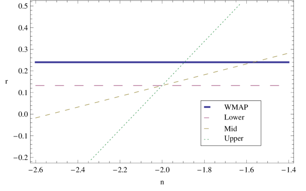
Figure 1: Plot of the scalar-tensor ratio as a function of power law index $n$. The WMAP bound implies that only values of n $\in(-2.4,-1.6)$ are physically acceptable. The lower bound arises because a physical $r$ must be non-negative.

As one can see, the lower bound implies a vanishing of the $P_{A}^{2}$ term and therefore a constant value of $r$ which is below the WMAP bound. This is to be expected, since this is just canonical inflation. For non-zero values of the $P_{A}$ term up to the maximal, we see that there is a small window where $r$ satisfies the WMAP bound, and is positive definite.

Values of $n$ outside the identified range are incompatible with observation, or non-physical therefore should be ruled out as viable candidates for inflation. As expected from our earlier observation of the Hamilton-Jacobi equation, the theory with $n=-2$ is indistinguishable from inflation without gauge field (at leading order) and therefore easily satisfies the WMAP constraint.

One could examine the entire parameter space to classify the inflating trajectories in terms of the BI functions, however this is not the main focus of this paper, and we leave the full parameter space evaluation for future work. We comment briefly on the case of exponential coupling $b(\phi)\sim Ae^{a\phi^{2}}$, $a$ is a constant, (cf. 2.24) which may be of interest. In this case the scalar field admits the following perturbative solution

$$\phi(\alpha)\sim\sqrt{\phi_{0}^{2}-4\alpha M_{p}^{2}}\left(1-\frac{e^{-\phi_{0}^{2}/M_{p}^{2}}P_{A}^{2}}{2m^{2}(\phi_{0}^{2}-4\alpha M_{p}^{2})}\left(Ei\left(\frac{\phi_{0}^{2}}{M_{p}^{2}}\right)+Ei\left(\frac{\phi_{0}^{2}-4\alpha M_{p}^{2}}{M_{p}^{2}}\right)-2\alpha M_{p}^{2}e^{-4\alpha+\phi_{0}^{2}/M_{p}^{2}}\right)\right)$$ (2.33)

where $Ei(x)$ is the ExpIntegralEi(x) function [31], and the field satisfies the usual boundary condition that $\phi(0)=\phi_{0}$. Note that this solution differs from that in (2.25) through the use of the Ei function. We will now turn to a related issue, examining how gauge fields interact with the DBI theory of $D3$-branes.

3 D-Brane theory

As briefly mentioned in sections 1 and 2, the non-linearity type of structure present in the Born-Infeld frameworks turns out to provide the correct low energy description of $Dp$-branes in string theory. In this context a class of models within type IIB string cosmology, more often referred to as DBI-cosmology has been considered . Notwithstanding their interest, the simplest models of DBI-cosmology are plagued by several issues which disfavor them as inflationary candidates [37, 38, 39]. More complex models can be constructed which circumvent these issues, but they all appear sensitive to supergravity back-reaction in the relativistic limit [38, 40, 41]. All these particular models make use of internal spaces that are asymptotically AdS, and it has not yet been established whether more general backgrounds are more viable. Recently the non-trivial coupling between dilaton and gauge field has been exploited in [42] through the use of Wilson lines: Inflation in such a model appears to avoid several of the pathologies of previous DBI inflation, and suggests that such non-trivial couplings are important to realise an inflationary phase. Since such non-trivial couplings are generated through non-AdS backgrounds, our aim in what follows is to consider such geometries in the hope that they can be embedded into the full string theory. Throughout this section we will discuss how some simpler (Lagrangian) configurations can be of interest. We will show how we can compute modifications on the scalar field dynamics (and hence, the inflationary universe), given constraints on the electromagnetic energy density. More concretely, we will investigate specific limits of the equations of motion; Namely the non-relativistic and relativistic limit (cf. subsections 3.1 and 3.2, respectively). These will allow us to establish backreaction situations of gauge fields on the inflaton and possibly identify cosmological implications, namely observational. The feature to stress is that the allowed couplings induce herein a much richer class of dynamical possibilities than the content in section 2 (A brief discussion on generating magnetic seed fields suitable for these limits is first presented in Appendix A.).

Let us start with the following effective theory for DBI cosmology for a single $D3$-brane (which is in Einstein frame), where we include a scalar potential which does not come from the world-volume calculation but could arise from a supergravity F-term,

$$S=\int d^{4}x\left(-F_{1}(\phi)\sqrt{-{\rm det}(G_{\mu\nu}+F_{3}(\phi)F_{\mu\nu})}+q\sqrt{-g}F_{1}(\phi)-\sqrt{-g}V(\phi)\right),$$ (3.1)

where the induced metric is

$$G_{\mu\nu}=g_{\mu\nu}+F_{2}(\phi)\partial_{\mu}\phi\partial_{\nu}\phi$$ (3.2)

and $q$ is a measure of the RR-charge carried by the brane, where $q=1$ for a BPS $D3$-brane, $q=-1$ for a $\bar{D}3$-brane and $q=0$ corresponds to non-BPS branes such as employed in models of tachyon dynamics. We will assume that $F_{1}$ is non-negative for simplicity. Negative tension objects must exist for a string compactification to be consistent, but we will not consider them in this particular paper. The bulk metric $g_{\mu\nu}$ is assumed to be a solution of type IIB string theory in Einstein frame. Our ansatz (2.2) is, in fact, general enough to extend to these backgrounds which typically have a non-trivial dilaton profile - which is important because the determinant contains additional powers of the dilaton, coupling to the Maxwell tensor in Einstein frame. Backgrounds falling into this class can be found in [43, 44].

One can calculate the determinant at leading order and therefore can write the above action as follows

$$S=\int d^{4}x\left(-F_{1}(\phi)\sqrt{-G}\left(1+\frac{1}{4}F_{3}^{2}(\phi)F_{\mu\nu}F^{\mu\nu}\right)+\sqrt{-g}(qF_{1}(\phi)-V(\phi))\right),$$ (3.3)

where indices are raised and lowered with the full metric $G_{\mu\nu}$ rather than $g_{\mu\nu}$. Note that we are neglecting any couplings to the axion, which in this theory could come in the form $c_{0}F\wedge F$. The $F_{i}$ are functions of the scalar embedding, arising from placing the $D3$-brane in the non-trivial geometry. The factors of the brane tension are contained in the $F_{1}$ parameter. This action appears superficially similar to that of Einstein-Maxwell theory, which typically has a coupling between scalar and gauge sectors as $b^{2}(\phi)F_{\mu\nu}F^{\mu\nu}$. In the D-brane theory we see that this coupling is fixed to be $F_{1}F_{3}^{2}$, which potentially allows for much richer solutions than the function $b(\phi)$. Note however that the Maxwell tensors also couple to the inflaton through the term $\sqrt{-G}$, which contain powers of $\dot{\phi}^{2}$. For dynamic solutions, this coupling explicitly breaks conformal invariance. Therefore even for theories with $F_{1}F_{3}^{2}=1$, the conformal structure of the gauge field sector is still broken [25].

The modified Klein-Gordon equation is much more complicated, but takes the following form

$$0 = \left(1+\frac{F_{3}^{2}}{4}F_{\mu\nu}F^{\mu\nu}\right)\left\{F_{1}F_{2}^{\prime}\dot{\phi}^{2}(1-4e^{3\alpha})-2F_{1}^{\prime}\left[1-F_{2}\dot{\phi}^{2}+\frac{e^{3\alpha}F_{1}F_{2}\dot{\phi}^{2}}{(1-F_{2}\dot{\phi}^{2})}\right]-6e^{3\alpha}\dot{\alpha}F_{1}F_{2}\dot{\phi}\right\}$$ (3.4)

$$- 2F_{1}F_{2}\ddot{\phi}e^{3\alpha}\left(1+\frac{F_{3}^{2}}{4}F_{\mu\nu}F^{\mu\nu}\right)-F_{1}F_{3}F_{3}^{\prime}\frac{F_{\mu\nu}F^{\mu\nu}}{2\sqrt{1-F_{2}\dot{\phi}^{2}}}\left(1-F_{2}\dot{\phi}^{2}+e^{3\alpha}F_{3}\dot{\phi}^{2}\right)$$

$$+ qF_{1}^{\prime}-V^{\prime}-\frac{e^{3\alpha}F_{1}F_{2}F_{3}^{2}\dot{\phi}}{4\sqrt{1-F_{2}\dot{\phi}^{2}}}\frac{\partial}{\partial t}(F_{\mu\nu}F^{\mu\nu}),$$

where a dot denotes a time derivative, and primes denote herein scalar field derivatives. For backgrounds which are asymptotically $AdS$, the string and Einstein frames coincide - leading to a theory with a trivial dilaton (at leading order). Canonical examples of such theories include;

• $F_{1}=F=\phi^{4}/\lambda,F_{2}=f,F_{3}=1/\sqrt{F},q=\pm 1$ for the AdS solution;

• $F_{1}=V(\phi),F_{2}=1,F_{3}=\lambda,q=0$ for the tachyon solution [45, 46, 47, 48]

We must now consider the Einstein equations for such a configuration. These will generally be complicated by the presence of the induced metric $G$ rather than the space-time metric $g$. Using the variational identity

$$\delta G^{ab}=\delta g^{ac}(\delta^{c}_{b}+g^{ce}h_{eb})^{-1}-\delta g^{\mu\nu}g^{ac}h_{\nu\sigma}(\delta^{\mu}_{b}+g^{\mu x}h_{xb})^{-1}(\delta^{c}_{\sigma}+g^{c\rho}h_{\rho\sigma})^{-1},$$ (3.5)

one can calculate the corresponding energy momentum tensor to be

$$T_{\mu\nu} = -\frac{1}{4}\sqrt{1-F_{2}\dot{\phi}^{2}}F_{1}F_{3}^{2}F_{ab}F^{ab}\left(G_{\mu b}(\delta^{\nu}_{b}+g^{\nu e}h_{eb})^{-1}-G_{ab}g^{ac}h_{\nu\sigma}(\delta^{\mu}_{b}+g^{\mu e}h_{eb})^{-1}(\delta^{c}_{\sigma}+g^{ce}h_{e\sigma})^{-1}\right)$$ (3.6)

$$+ \frac{1}{2}F_{1}F_{3}^{2}\sqrt{1-F_{2}\dot{\phi}^{2}}\left(F_{\mu b}F_{cd}G^{bd}(\delta^{\nu}_{c}+g^{\nu e}h_{ec})^{-1}+F_{a\mu}F_{cd}G^{ac}(\delta^{\nu}_{b}+g^{\nu e}h_{eb})^{-1}\right)$$

$$- \frac{1}{2}\sqrt{1-F_{2}\dot{\phi}^{2}}h_{\nu\sigma}(\delta^{l}_{\sigma}+g^{le}h_{e\sigma})^{-1}\left(G^{bd}g^{al}(\delta^{\mu}_{c}+g^{\mu f}h_{fc})^{-1}+G^{ac}g^{bl}(\delta^{\mu}_{d}+g^{\mu k}h_{kd})^{-1}\right)$$

$$+ F_{1}\sqrt{1-F_{2}\dot{\phi}^{2}}\left(-G_{\mu b}(\delta^{\nu}_{b}+g^{\nu e}h_{eb})^{-1}+G_{ab}g^{ac}h_{\nu\sigma}(\delta^{\mu}_{b}+g^{\mu e}h_{eb})^{-1}(\delta^{c}_{\sigma}+g^{cf}h_{f\sigma})^{-1}\right)$$

$$+ g_{\mu\nu}(qF_{1}-V),$$

where we have defined $h_{ab}=F_{2}\partial_{a}\phi\partial_{b}\phi$ for simplicity. Since the DBI action has a well-defined relativistic limit, we choose to define $\gamma\equiv(1-F_{2}\dot{\phi}^{2})^{-1/2}$ as the analog of the ‘gamma’ factor in special relativity. The resulting Einstein equations arising from the Bianchi metric, can then be written as follows

$$\dot{\alpha}^{2}-\dot{\sigma}^{2} = \frac{1}{3M_{p}^{2}}\left(F_{1}(\gamma-q)+V+\frac{F_{1}F_{3}^{2}\gamma^{3}\dot{A_{x}^{2}}e^{-2\alpha+4\sigma}}{2}\right),$$ (3.7)

$$\ddot{\sigma}+3\dot{\alpha}\dot{\sigma} = \frac{e^{-2\alpha+4\sigma}F_{1}F_{3}^{2}\dot{A_{x}^{2}}\gamma(\gamma^{2}+1)}{6M_{p}^{2}},$$ (3.8)

$$2\ddot{\alpha}+3\dot{\alpha}^{2}+3\dot{\sigma}^{2} = \frac{1}{M_{p}^{2}}\left(\frac{F_{1}(1-\gamma q)}{\gamma}+V-\frac{e^{-2\alpha+4\sigma}F_{1}F_{3}^{2}\dot{A_{x}^{2}}\gamma(2\gamma^{2}-1)}{6}\right)$$ (3.9)

and one finds that the equation for an accelerating universe is given by

$$\frac{\ddot{a}}{a}=-2\dot{\sigma}^{2}+\frac{1}{3M_{p}^{2}}\left(\frac{F_{1}(3-2\gamma q-\gamma^{2})}{2\gamma}+V-\frac{e^{-2\alpha+4\sigma}F_{1}F_{3}^{2}\dot{A_{x}^{2}}\gamma(3\gamma^{2}-1)}{4}\right).$$ (3.10)

From the right hand side of this equation one sees that the energy density of the vector field is important when considering inflationary dynamics. Indeed we can identify a critical value of the gauge field which allows for acceleration (isotropic limit):

$$\dot{A_{x}^{2}}<\frac{4e^{2\alpha-4\sigma}}{F_{1}F_{3}^{2}\gamma(3\gamma^{2}-1)}\left(V-\frac{F_{1}(\gamma^{2}+2\gamma q-3)}{2\gamma}\right).$$ (3.11)

Note that in DBI inflation, the scalar potential dominates the energy density even for relativistic rolling. It can then be seen that the term on the right hand side is a decreasing function as one approaches the relativistic limit. This reduces the solution space for $\dot{A}_{x}^{2}$ so that it approaches zero as $\gamma\to\infty$.

Finally upon variation of the action we find the coupled Maxwell equation

$$\partial_{\mu}\left(\sqrt{-G}F_{1}(\phi)F_{3}^{2}(\phi)F^{\mu\nu}\right)=0,$$ (3.12)

which mixes the inflaton with the gauge field. Inserting our ansatz from section 2.1 we find that the equation becomes

$$\ddot{A}_{x}+\dot{A}_{x}\left(\dot{\alpha}+4\dot{\sigma}+\frac{F_{1}^{\prime}}{F_{1}}\dot{\phi}+\frac{2F_{3}^{\prime}}{F_{3}}\dot{\phi}+\frac{F_{2}^{\prime}\dot{\phi}^{3}}{(1-F_{2}\dot{\phi}^{2})}+\frac{2F_{2}\dot{\phi}\ddot{\phi}}{(1-F_{2}\dot{\phi})}\right)=0.$$ (3.13)

Solutions to the Maxwell equation include the following - similar to that in the BI-theory

$$\dot{A}_{x}\simeq-\frac{P_{A}e^{-\alpha-4\sigma}}{\gamma F_{1}F_{3}^{2}},$$ (3.14)

where we denote the constant of integration as $P_{A}$. In this case $P_{A}$ is a measure of the charge carrier density on the world-volume because the gauge field arises from excited states of open $F$-strings that end on the brane.

In the non-relativistic limit $(\gamma\sim 1)$, the scalar potential will effectively dominate the right hand side of the constraint equation (3.11). Therefore for a sufficiently ‘large’ potential, this condition can easily be satisfied. In the ultra-relativistic limit, the right hand side is proportional to $\gamma^{-3}(V-\gamma F_{1}/2)$ which may not be very large without fine-tuning, thereby making the constraint equation (3.11) very difficult to satisfy. Clearly the gauge field will have the most dramatic effect on relativistic inflation, but may also play an important role in the non-relativistic limit. We can again, like in subsection 2, adapt the constraint on the energy density during inflation, in the form of a ratio of energy densities to be approximately constant (cf., e.g., (2.17)). In the case of the DBI theory, the new expression for the ratio takes the form

$$\mathcal{R}=\frac{P_{A}^{2}\gamma e^{-4\alpha-4\sigma}}{2F_{1}F_{3}^{2}(F_{1}(\gamma-q)+V)},$$ (3.15)

which clearly relates the various parameters in the model. Examining the ratio (3.15) for sufficiently small values of $\dot{\phi}$ - and considering the critical limit where the gauge field energy density is almost constant during inflation - we find the constraint

$$F_{1}F_{3}^{2}\sim e^{-4\alpha},$$ (3.16)

which is the generalised extension of the known results from Einstein-Maxwell theory. To further assist in understanding the role of the gauge field, we use the parameter $c$ (cf. Appendix A), which conveys the deviation from the above result. More precisely, the solution we must consider is $F_{1}F_{3}^{2}\sim e^{-4ac}$ - which is the most general expression. For $c>1$, the gauge field terms will rapidly come to dominate the dynamics at late times.

Before proceeding and specializing with different settings of our DBI framework, let us indicate that the anisotropies are governed (at leading order) by equations (3.7), (3.8) above. Under the assumption that they are small, and obey slow-roll behaviour, we can immediately write down the relevant Hamilton-Jacobi equation which describes their dynamics

$$\frac{d\sigma}{d\alpha}\sim\left(\frac{P_{A}^{2}}{F_{1}F_{3}^{2}}\right)\left(\frac{1+\gamma^{2}}{6\gamma}\right)\frac{e^{-4\alpha}}{F_{1}(\gamma-q)+V}.$$ (3.17)

In the non-relativistic limit, the $\gamma$ terms reduce to a constant (given by $1/3$), and the magnitude is then set by whichever term dominates the scalar energy density. For ultra relativistic motion, the middle term appears to be linear in $\gamma$, and if the scalar potential is dominant this suggests that the anisotropies may be large. However if the $F_{1}\gamma$ term dominates the energy density, then the $\gamma$ factors actually cancel - and the anisotropies are then determined by the new term $F_{1}^{2}F_{3}^{2}$.

3.1 Non-Relativistic limit

The non-relativistic limit of the theory emerges when $\gamma\sim 1+\frac{1}{2}F_{2}\dot{\phi}^{2}+\ldots$. Although this is a modified version of slow-roll inflation, there is a non trivial coupling to the gauge field and therefore one may expect back-reaction to be an issue. Note that for $q=1$ the effective potential $V_{eff}=V(\phi)+F_{1}(\phi)(1-q)$ reduces to the scalar potential due to supersymmetry, and when $q=0$ we have a purely non-BPS system - which also allows for $V=0$ and the dynamics are dictated by $F_{1}$ alone.

Expanding the DBI Lagrangian to leading order yields a corresponding effective field equation

$$\ddot{\phi}+3\dot{\alpha}\dot{\phi}+\dot{\phi}\frac{\dot{Q}}{Q}-\frac{W^{\prime}}{Q}-\frac{\dot{\phi}^{2}}{2}\frac{Q^{\prime}}{Q}=0,$$ (3.18)

where herein dots denote time derivatives, primes are derivatives with respect to the scalar field and we employ the following variable definitions

$$Q \equiv F_{1}F_{2}\left(1+\frac{F_{3}^{2}}{4}F_{\mu\nu}F^{\mu\nu}\right)=F_{1}F_{2}\left(1-\frac{x}{2}\right),$$ (3.19)

$$W \equiv F_{1}(q-1)-V-F_{1}\frac{x}{2},$$ (3.20)

where $x\equiv-\frac{F_{3}^{2}}{2}F_{\mu\nu}F^{\mu\nu}$. We have not made any assumptions about the background geometry at this stage, and this result is therefore quite robust. Let us study the background evolution by starting with the isotropic inflationary limit and initially set the gauge field and $\ddot{\phi}$ terms to zero, in which case the above equation of motion reduces to

$$3\dot{\alpha}\dot{\phi}+\frac{\dot{\phi}^{2}}{2}\frac{\partial}{\partial\phi}\ln(F_{1}F_{2})-\frac{(q-1)}{F_{2}}\frac{\partial}{\partial\phi}\ln(F_{1})+\frac{V^{\prime}}{F_{1}F_{2}}\sim 0,$$ (3.21)

which is reminiscent of a canonically coupled scalar field solution - except that there is an additional driving term proportional to $\dot{\phi}^{2}$. Note that BPS configurations ($q=1$ in our language) simplify the equation of motion significantly since the second term in (3.21) vanishes in this limit (with the usual assumptions about regularity of the background function). The troublesome $\dot{\phi}^{2}$ terms, which have no analog in canonical slow roll models, will always contribute - unless we can consider limits where $F_{1}F_{2}$ is constant. This amounts to localising the solution on a curve in parameter space, and is what we consider in this paper. General solutions to the above equation will be explored in the future.

3.1.1 $F_{1}F_{2}$ Constant

With the assumption that $F_{1}F_{2}$ is constant, the field equation becomes a modified version of the canonical scalar field equation. We can immediately write down the scale factor as a function of the inflaton using the Hamilton-Jacobi formalism, for an arbitrary scalar potential

$$\alpha=-\frac{F_{1}F_{2}}{M_{p}^{2}}\int\frac{V}{V^{\prime}}d\phi.$$ (3.22)

For a simple chaotic inflationary potential such as $\frac{1}{2}m^{2}\phi^{2}$ theory, we can then see that the back-reaction constraint (3.16) implies the following general relationship

$$F_{1}F_{3}^{2}\sim\exp\left(\frac{F_{1}F_{2}c\phi^{2}}{M_{p}^{2}}\right).$$ (3.23)

which dictates the functional form of $F_{3}$, given that $F_{1}$ is fixed.

We now proceed to include the gauge field terms in the modified Klein-Gordon equation which we write as a perturbative expansion in $x$, and takes the general form

$$0 \sim 3\dot{\alpha}\dot{\phi}\left(1+\frac{2x}{3}\right)+\frac{\dot{\phi}^{2}}{2}\frac{\partial}{\partial\phi}\ln(F_{1}F_{2})+\frac{V^{\prime}}{F_{1}F_{2}}\left(1+\frac{x}{2}\right)$$ (3.24)

$$+ \frac{(x-(x+1)(q-1))}{2F_{2}}\frac{\partial}{\partial\phi}\ln(F_{1})+\frac{x(F_{2}\dot{\phi}^{2}-2)}{2F_{2}}\frac{\partial}{\partial\phi}\ln(F_{1}F_{3}),$$

although the $\dot{\phi}^{2}$ term in the last bracket in the expression above is actually subleading in the non-relativistic expansion - and can be neglected. Note that the source term also appears to be coupled to the scalar potential, which is due to the non-canonical nature of the theory. To solve this equation, we use the energy density constraint (3.15) to solve for $F_{3}$ under the assumption of a quadratic scalar potential - since this is the simplest analytic solution. One can solve this equation numerically, however we present only analytic solutions in this paper - leaving a more exhaustive analysis to future work:

(a) Let us initially consider $F_{1}$ to be constant, which (by assumption) implies that $F_{2}$ is also constant. Using the back-reaction condition to solve for $F_{3}$ we can then find the solution to the scalar field equation in the presence of the gauge field. At late times the solution can be calculated to converge to the following

$$e^{-4\alpha-F_{1}F_{2}c\phi^{2}/M_{p}^{2}}\sim\frac{6(c-1)F_{1}m^{2}M_{p}^{2}}{cP_{A}^{2}(6F_{1}^{2}F_{2}c-m^{2}M_{p}^{2})},$$ (3.25)

where the right hand side is clearly a constant which vanishes for $c=1$, therefore the electromagnetic energy density will also be constant. We see that $F_{1}F_{3}^{2}\sim 1/a^{2}$ in the regime where $P_{A}$ is constant, but more importantly it highlights the fact that $c\sim 1$ as the back-reaction becomes relevant.

For a canonically coupled field, there is attractor behavior since the gauge field energy density exhibits tracking behaviour [18]. In our case, due to the non-canonical nature of the action, the source term in the field equations also couples to the scalar potential. If we demand that the scalar and gauge fields are effectively the same magnitude, so that they are both source terms in the field equation, then we find

$$m^{2}M_{p}^{2}\sim\frac{xc(F_{1}F_{2})^{2}}{F_{2}M_{p}^{2}}\left(1+\frac{x}{6}\right)$$ (3.26)

at leading order. Inserting this into the relation (3.15) we discover that

$$\mathcal{R}\sim\frac{M_{p}^{2}}{c\phi^{2}(F_{1}F_{2})}.$$ (3.27)

Given that inflation occurs for $\phi\sim\mathcal{O}(10)M_{p}$ in this model, we find $\mathcal{R}\sim x10^{-2}/(F_{1}F_{2})$, which can be vanishingly small for sufficiently large $F_{1}F_{2}$. This ensures that the gauge field energy density is negligible when compared to the scalar energy density and therefore we can consistently neglect its contribution to the Hubble parameter. Note that this is almost the same result as obtained in canonical models, aside from the factor of $F_{1}F_{2}$. This ensures that $\mathcal{R}\sim x10^{-2}/(F_{1}F_{2})$ is an attractor solution. If $\mathcal{R}$ is initially smaller than this, the behaviour of the scalar field drives $\rho_{A}$ to increase (with $c>1$), reaching this value from below. For configurations where this quantity is larger than the attractor solution, the inflaton can climb back up the scalar potential (due to the source term in the equation of motion). Thus $\rho_{A}$ is forced to decrease rapidly, and the attractor is reached from above. This confirms that even this non-canonical model we expect tracker behaviour.

As far as the anisotropies are concerned, dropping the $\ddot{\sigma}$ term in the anisotropic equation of motion (3.8), combined with the back-reacted solution implies the following

$$\frac{\dot{\sigma}}{\dot{\alpha}}\sim\frac{2P_{A}^{2}}{3m^{2}\phi^{2}}\frac{6(c-1)F_{1}m^{2}M_{p}^{2}}{cP_{A}^{2}(6F_{1}^{2}F_{2}c-m^{2}M_{p}^{2})},$$ (3.28)

indicating that anisotropies increase during this accelerated phase for $c>1$ and $6cF_{1}^{2}F_{2}>m^{2}M_{p}^{2}$. Of course, in order to determine this result we assume a perturbative $\sigma$ as before. Note that, as in the case of Born-Infeld theory, the increase in anisotropy is determined by the scalar potential. Both solutions (2.14) and (3.28) increase like $1/\phi^{2}$ - although in the latter case the anisotropies also vanish when $c=1$.

(b) Consider now a regime of solution space where the logarithmic terms dominate in the back-reacted equation of motion - still assuming that $F_{1}F_{2}$ is constant. The solution for the scalar field in this instance becomes

$$e^{-4\alpha-F_{1}F_{2}c\phi^{2}/M_{p}^{2}}\sim\frac{e^{-4\alpha}m^{2}M_{p}^{2}}{nF_{1}^{2}F_{2}^{2}c^{2}P_{A}^{2}(1-e^{-4\alpha})+m^{2}M_{p}^{2}e^{F_{1}F_{2}c\phi_{0}^{2}/M_{p}^{2}}},$$ (3.29)

where $n$ is an integer depending on whether $F_{1}(n=1)$ or $F_{3}(n=2)$ is fixed to be constant. Note that this is similar to the result obtained in (3.25) with the additional dependence on the scale factor appearing on the right hand side which ensures the solution decreases as a function of time. The scale factor dependence arises precisely because of this logarithmic running. The solutions are valid in a regime where the scalar mass in the quadratic potential satisfies the following bound

$$m^{2}<<\frac{nxcF_{1}^{2}F_{2}}{M_{p}^{2}}\left(1-\frac{x}{6}\right)$$ (3.30)

where $n$ is defined as above, and when $n=2$ we must recall that $F_{1}$ depends on the inflaton. This bound can be satisfied for a (small) region of solution space and is therefore a physical solution. If the parameters are chosen so as to satisfy this bound, then one can easily show that for initially small anisotropies, these are actually decreasing during the inflationary expansion - indicating that the isotropic universe would be a late time attractor.

(c) It is also of interest to explore a solution branch where we fix the functional form of $F_{3}$, but with the same assumption that the logarithmic terms are dominant with respect to the scalar potential. This should then modify the above result for the scalar field. The ansatz we select is $F_{3}\sim L\phi^{a}$ - which allows us to find the analytic solution

$$e^{-4\alpha-cF_{1}F_{2}\phi^{2}/M_{p}^{2}}\sim\frac{m^{2}M_{p}^{2}e^{-4\alpha}}{F_{1}^{2}F_{2}^{2}c^{2}P_{A}^{2}(1-e^{-4\alpha})+m^{2}M_{p}^{2}e^{F_{1}F_{2}c\phi_{0}^{2}/M_{P}^{2}}},$$ (3.31)

which is in fact identical to the solution above for $n=1$. This suggests that the anisotropies are decreasing in this regime - since their overall magnitude is a decreasing function of $\alpha$. Let us therefore consider a solution where $F_{1}\sim L\phi^{a}$ - which continues to fix $F_{2}$, but now with $F_{3}$ as a constant. The resulting expression for the back-reacted field equation is

$$\phi^{\prime}(\alpha)\sim\frac{2F_{1}F_{2}cP_{A}^{2}}{m^{2}}e^{-4\alpha-F_{1}F_{2}c\phi^{2}/2M_{p}^{2}}$$ (3.32)

which admits a complicated solution of the form

$$e^{-cF_{1}F_{2}\phi^{2}/M_{p}^{2}}\sim\exp\left(2{\rm InverseErf}\left(i{\rm Erfi}\left[\frac{\phi_{0}}{M_{p}}\sqrt{\frac{F_{1}F_{2}c}{2}}\right]+\frac{i(F_{1}F_{2}c)^{3/2}P_{A}^{2}(1-e^{-4\alpha})}{m^{2}M_{p}\sqrt{2\pi}}\right)^{2}\right),$$

where $Erfi$ is the imaginary error function [31] and therefore one sees that even for $c=1$ there are non-trivial contributions to the anisotropy equation.

(d) We have considered the equation of motion where the logarithm terms were dominant, but more physically for the non-relativistic case, we can anticipate the scalar potential to be the largest contributor to energy density. We may again choose to set either $F_{1}$ or $F_{3}$ fixed to be constant, which leads to the resulting expressions shown below;

$$e^{-4\alpha-cF_{1}F_{2}\phi^{2}/M_{p}^{2}} \sim \frac{2F_{1}(1-c)}{cP_{A}^{2}}\hskip 22.76228pt(F_{3})$$ (3.33)

$$\sim \frac{(1-2c)e^{-2\alpha}}{P_{A}F_{3}\sqrt{c}}\hskip 14.22636pt(F_{1}).$$

The first solution is constant for constant $F_{3}$ and clearly vanishes for $c=1$. The second solution is for constant $F_{1}$, but clearly decreases with time. Moreover the solution does not vanish for $c=1$, rather it vanishes for $c=1/2$ - indicating that anisotropies will be increasing in this case.

3.1.2 $AdS_{5}$ Solution

As an example of a particular solution, let us consider the case of a pure $AdS_{5}$ embedding, generated by $N$ coincident $D3$-branes at large $N$. The background functions must now satisfy the following expressions $F_{1}=\phi^{4}/\lambda^{2},F_{3}=1/\sqrt{F_{1}}$ and $F_{2}$ is constant. Since the background functions are explicitly known, the gauge coupling is fixed - in fact it is unity which leads to a trivial result. The solutions depend explicitly upon the particular brane being embedded into the theory.

We focus initially on non-BPS configurations where $q\neq 1$. In this case, we must ensure that $\lambda>>1$ for analytic solutions. We will again assume that the scalar potential is quadratic. With the gauge field set to zero, we find the equation of motion at leading order in $\lambda$ becomes

$$\phi^{\prime}(\alpha)\sim-\frac{2M_{p}^{2}\lambda^{2}}{F_{2}\phi^{5}}+\ldots,$$ (3.34)

where the higher order terms are sub-leading in $\lambda^{2}$. The above equation admits the following solution

$$\phi^{6}(\alpha)\sim\phi_{0}^{6}-\frac{12\alpha\lambda^{2}M_{p}^{2}}{F_{2}}$$ (3.35)

where we neglect the sub-leading terms in $\lambda$. This leads to a cancellation of the scalar field mass in the equation of motion, therefore the solution does not appear to depend on it at leading order. The corrections coming from the gauge field lead to the following master equation

$$\phi^{\prime}(\alpha)\sim-\frac{2M_{p}^{2}\lambda^{2}}{F_{2}\phi^{5}}\left(1-\frac{\lambda^{4}P_{A}^{2}e^{-4\alpha}}{\phi^{4}}\right),$$ (3.36)

which must be solved perturbatively. Let us define $\phi\equiv\chi+P_{A}^{2}\xi+\ldots$ at leading order - where the solution for $\chi$ is the one found above in (3.35). The back-reacted solution therefore has the leading order solution

$$\phi(\alpha)\sim\chi\left(1+\frac{\lambda^{2}e^{-F_{2}\phi_{0}^{6}/(3\lambda^{2}M_{p}^{2})}}{36\chi^{4}}\left\{\tilde{E}\left[\frac{2}{3},-\frac{F_{2}\chi^{6}}{3\lambda^{2}M_{p}^{2}}\right]-\frac{\phi_{0}^{2}}{\chi^{2}}\tilde{E}\left[\frac{2}{3},-\frac{F_{2}\phi_{0}^{6}}{3\lambda^{2}M_{p}^{2}}\right]\right\}\right),$$ (3.37)

where we use the short-handed notation $\widetilde{E}[x,y]=\rm{ExpIntegralE}[x,y]$ for simplicity [31]. Note that the boundary conditions ensure that $\phi\sim\phi_{0}$ at $\alpha=0$. Since both $F_{1}$ and $F_{3}$ are defined by the background geometry in this instance, we may find it hard to satisfy our gauge density constraint (3.15). Indeed, one can see that $\mathcal{R}$ only depends on the ratio $e^{-4\alpha}/\phi^{2}$ which cannot be constant at this order of approximation.

In the case of $q=1$, which is the BPS configuration (in the static limit) we now need to assess whether we keep the $\dot{\phi}^{2}$ terms in the equation of motion. If we set them to zero, then we recover the expression (3.34) as an exact result, not a perturbative one. The back-reacted solution will also then follow trivially. Instead let us keep the quadratic terms in the equation of motion. We can then solve this equation in the absence of a gauge field to obtain the expression

$$\dot{\phi}\sim-\frac{3\dot{\alpha}\phi}{2}+\ldots,$$ (3.38)

where we must ensure that the following condition is satisfied

$$1>>\frac{3F_{2}\phi^{6}}{16\lambda^{2}M_{p}^{2}}.$$ (3.39)

This can be done if we also assume $\lambda^{2}>>1$, which is good for the supergravity approximation. In this limit of the theory we find that dynamic solutions are exponentially decaying

$$\phi\sim\phi_{0}e^{-3\alpha/2}$$ (3.40)

and if one includes the backreaction at leading order, the solution is

$$\phi(\alpha)\sim e^{-3\alpha/2}\left(\phi_{0}^{4}\pm\lambda^{2}P_{A}^{2}(1-e^{2\alpha})\right)^{1/4},$$ (3.41)

where we must again impose the constraint condition (3.39). Intuitively these results make sense, because we are forced to consider a perturbative expansion in the mass term, which effectively decouples the scalar potential from the theory. The scalar field is driven purely by the potential generated by the AdS background.

The energy density ratios in the two cases of interest may be written

$$\mathcal{R}_{1}\sim\frac{P_{A}^{2}\lambda^{3}}{m^{2}\phi^{6}}\left(\frac{\phi_{0}}{\phi}\right)^{8/3},\hskip 28.45274pt\mathcal{R}_{2}\sim\frac{P_{A}^{2}\lambda^{3}}{m^{2}\phi^{6}}\left(1-\frac{F_{2}(\phi_{0}^{6}-\phi^{6})}{3\lambda^{2}M_{p}^{2}}\right),$$ (3.42)

where $\mathcal{R}_{1}$ is the solution arising when we neglect $\dot{\phi}^{2}$ terms in the equation of motion. Note that $\mathcal{R}_{1}$ is initially very small, but increasing during inflation indicating that the energy density of the gauge field is highly suppressed. As $\phi$ continues to decrease, corresponding to the limit where the probe branes are nearing the $D3$-branes, the ratio rapidly starts to diverge indicating that the gauge field contribution overwhelms the scalar energy density and back-reaction dominates. The solution for $\mathcal{R}_{2}$ also increases as the brane approaches the stack, although one must be careful to ensure that the parameters satisfy the constraint (3.39). One notes that, when compared to $\mathcal{R}_{1}$ with similar choices of parameters, that $\mathcal{R}_{2}$ is significantly smaller in magnitude than $\mathcal{R}_{1}$, and the gauge field domination occurs at later times.

Regarding the anisotropies we see that herein the equation of motion in the BPS case $q=1$ (dropping the $\dot{\phi}^{2}$ terms) can be written as follows;

$$\frac{\dot{\sigma}}{\dot{\alpha}}\sim\frac{4P_{A}^{2}\lambda^{3}}{3m^{4}\phi^{8}}\left(\frac{\phi_{0}}{\phi}\right)^{8/3},$$ (3.43)

which are increasing rapidly in this instance due to the exponentially decaying behaviour of the scalar field. In the case where we neglect the $\dot{\phi}^{2}$ terms, the solution becomes

$$\frac{\dot{\alpha}}{\dot{\sigma}}\sim\frac{4P_{A}^{2}\lambda^{2}}{3m^{4}\phi^{8}}\left(1-\frac{F_{2}(\phi_{0}^{6}-\phi^{6})}{3\lambda^{2}M_{p}^{2}}\right),$$ (3.44)

at leading order in $\lambda$ for all $q$. The result is that the anisotropies are increasing during inflation, recalling that the parameter space is tightly constrained, and at a smaller level than the previously considered solutions.

3.1.3 Tachyonic solution

Let us consider the non-relativistic expansion for the tachyonic solution in a non-BPS configuration, where $F_{2}$ is a constant, $F_{1}$ is the tachyon potential and $q=0$. We will take the potential to be of the form $F_{1}\sim V_{0}/\cosh(\phi/L)$, where $L$ is an unknown dimensionful parameter. We leave this arbitrary because it is highly likely that the tachyon potential in curved space is different from the one derived using BSFT (Boundary String Field Theory) in flat space . Additionally we will also set the scalar potential to zero, ensuring that the inflaton dynamics is driven only by open string condensation on the world-volume. The resulting ratio constraint from (3.15) becomes

$$F_{1}^{2}F_{3}^{2}\sim Z^{2}e^{-4\alpha c},$$ (3.45)

where $Z$ is a dimensionful parameter of the theory (cf. Appendix).

The background field equation with the above tachyonic potential results in the following expression for the inflaton

$$\tanh\left(\frac{\phi}{2L}\right)\sim\exp\left(\frac{\alpha M_{p}^{2}}{2F_{2}L^{2}V_{0}}\right),$$ (3.46)

where we have dropped the constants of integration. It is well known that tachyonic inflation requires severe fine-tuning, however the literature has have always assumed the validity of the flat space potential in curved space. Indeed when warping is taken into consideration, this fine tuning decreases allowing for potential inflationary trajectories [50]. In our case the warping is essentially embedded in the definition of $L$, which can lead to inflation when it is sufficiently large since it suppresses the mass of the inflaton.

The gauge coupling in this instance can be written as follows

$$F_{1}F_{3}^{2}\sim\frac{Z^{2}}{V_{0}}e^{-4\alpha c}\cosh\left(2\rm{arctanh}\left(e^{\alpha r}\right)\right),$$ (3.47)

where we defined $r\equiv M_{p}^{2}/(2F_{2}L^{2}V_{0})$. Note that this coupling is non-positive, and increasing towards zero from below. This is true even if the brane was a ghost brane, with negative tension. The backreacted equation of motion can be written as

$$\phi^{\prime}(\alpha)\sim-\frac{M_{p}^{2}}{2F_{2}}\left(1+\frac{4x}{3}\right)\frac{\partial}{\partial\phi}\ln F_{1},$$ (3.48)

which admits the following asymptotic solution

$$\tanh\left(\frac{\phi}{2L}\right)\sim\frac{1}{|\rm{coth}\left(\frac{\epsilon}{2L}\right)|}\exp\left(\frac{M_{p}^{2}(P_{A}^{2}(-1+e^{4\alpha(c-1)})+3\alpha(c-1)Z^{2}))}{6(c-1)F_{2}L^{2}V_{0}Z^{2}}\right),$$ (3.49)

where we have included the initial boundary condition on $\phi$ such that $\phi\to\epsilon<<L$ at $\alpha=0$. The gauge coupling is, in general, a rather complicated function of the scale factor

$$F_{1}F_{3}^{2}\sim\frac{Z^{2}e^{-4\alpha}}{V_{0}}\cosh\left(2\rm{arctanh}\left(tanh\left(\frac{\epsilon}{2L}\right)\exp\left(\frac{r}{3Z^{2}(c-1)}\left(P_{A}^{2}(-1+e^{4\alpha(c-1)})+3\alpha Z^{2}(c-1))\right)\right)\right)\right),$$ (3.50)

for arbitrary values of $c$; However, for $c=1$ the solution reduces to

$$F_{1}F_{3}^{2}\sim\frac{Z^{2}e^{-4\alpha}}{V_{0}}\cosh\left(2\rm{arctanh}\left(tanh\left(\frac{\epsilon}{2L}\right)\exp\left(\frac{r\alpha}{3Z^{2}}[4P_{A}^{2}+3Z^{2}]\right)\right)\right),$$ (3.51)

where $r$ is the same quantity defined earlier. Because of the perturbative correction in $P_{A}$ the gauge coupling for $c=1$ can be a positive, decreasing function (as a function of the expansion). However due to the algebraic structure of the solution, there is a critical value of the scale factor

$$\alpha_{c}=\frac{3Z^{2}}{r(4P_{A}^{2}+3Z^{2})}\ln\left(\rm{coth}\left(\frac{\epsilon}{2L}\right)\right)$$ (3.52)

at which the solution is singular, therefore we can only trust the solution for $\alpha<\alpha_{c}$. When the background is uniquely specified in this case, we see that decreasing solutions require $r<<1$. When we initially fix $r$, we then see that a decreasing gauge function requires $Z^{2}<<V_{0}$.

3.2 Relativistic limit

The relativistic limit occurs when $\gamma>>1$, corresponding to $\dot{\phi}^{2}\sim 1/F_{2}$, and the scalar equation of motion takes the following form

$$0 \sim F_{2}\gamma\dot{\phi}\left(1-\frac{x}{2}\right)\left(3\dot{\alpha}+\dot{\phi}\frac{\partial}{\partial\phi}\ln(F_{1})+\frac{\dot{\phi}(1+\gamma^{2}F_{2}\dot{\phi}^{2})}{2}\frac{\partial}{\partial\phi}\ln(F_{2})\right)$$

$$+ F_{2}\gamma\dot{\phi}x\left(2\dot{\alpha}+\dot{\phi}\frac{\partial}{\partial\phi}\ln(F_{1}F_{3})\right)+\frac{1}{\gamma}\left(1-\frac{x}{2}\right)\frac{\partial}{\partial\phi}\ln(F_{1})-\frac{x}{\gamma}\frac{\partial}{\partial\phi}\ln(F_{1}F_{3})+\frac{V^{\prime}-qF_{1}^{\prime}}{F_{1}}.$$

Since $\gamma$ is controlled by $F_{2}$, and we know the relation between this function and the inflaton, we will treat this as an unknown variable allowing us to eliminate the velocity from the problem. The equation of motion can then be solved once we specify the potential and the function $F_{1}$. Unlike the non-relativistic limit, there is no ‘trivial’ simplification that one can consider. The best approach turns out to be fixing the potential to be quadratic, as before, and assuming that $F_{1}$ satisfies power law behaviour, $F_{1}\sim L\phi^{p}$ where $L$ is herein a constant with mass dimension $(4-p)$.

In general, our assumption that $\gamma>>1$ allows us to solve the system explicitly once we specify $F_{2}$. To illustrate, let us assume that $F_{2}\sim\overline{W}\phi^{p}$. We can then integrate the equation of motion directly to obtain

$$\phi(t) \sim \frac{m}{M_{p}}\frac{1}{\sqrt{6}(p+4)}\left(\sqrt{W}\phi_{0}^{(2+p)/2}\left(\phi_{0}-\phi\right)+t\phi(2+p)\right),\hskip 28.45274ptp\neq-4$$ (3.54)

$$\sim \frac{\sqrt{T}\phi_{0}}{\sqrt{T}+t\phi_{0}},\hskip 221.93158ptp=-4$$ (3.55)

where $\overline{W},T$ are constants. We can then investigate the following cases:

(a) Let us assume that $V>>F_{1}q$ as a constraint on the Hubble equation. This is the limit in which (canonical) DBI-inflation can occur [51, 52]. Physically this corresponds to the inflaton being strongly damped by the Hubble factor, so that even though it is relativistic in velocity, it does not travel a large distance in field space. Knowing the scalar field solution, we can then use the Hubble equation to determine the scale factor

$$\alpha(\phi) \sim \frac{m}{M_{p}}\frac{1}{\sqrt{6}(4+p)}\left(\sqrt{T}\phi_{0}^{(2+p)/2}(\phi_{0}-\phi)+t\phi(2+p)\right),\hskip 28.45274ptp\neq-4$$ (3.56)

$$\sim \frac{m}{M_{p}}\sqrt{\frac{T}{6}}\ln\left(\frac{\phi_{0}}{\phi}\right),\hskip 182.09746ptp=-4$$ (3.57)

where we have assumed that $\phi$ is non-negative for simplicity - and imposed boundary conditions on the scale factor so that it vanishes at the start of inflation.

One could include the gauge field corrections to the above results, by employing the relevant term in the Hubble parameter. However it will turn out to be much simpler to use the scalar field equation to solve for $F_{2}$, and then compute the back-reaction on this variable. We will now consider this strategy where $F_{2}$ is unknown and $F_{1}$ has power law behaviour $F_{1}\sim L\phi^{p}$. The general equation is quite difficult to solve analytically once one includes the back-reaction. Therefore we illustrate the results for the case $p=2$, which has a leading order expansion of the form

$$F_{2}\sim\frac{2M_{p}^{2}\gamma^{4}(\nu_{2}-2)^{2}}{3m^{2}\phi^{4}}\left(1+\frac{2P_{A}^{2}}{3L\phi^{2}}\frac{(12+(\nu_{2}-2)(4c\pm 1))}{(4\gamma^{3}(c-1)(\nu_{2}+2)-3\nu_{2})}\left(\frac{\phi_{0}}{\phi}\right)^{4\gamma^{3}(c-1)(\nu_{2}-2)/3}\right),$$ (3.58)

where the $\pm$ sign arises from the particular choice of sign in the Hubble equation, and $\nu_{2}\equiv\frac{m^{2}}{\gamma^{3}L}$. One notes that the leading order dependence on the inflaton is $1/\phi^{4}$ and therefore one expects that the scale factor should initially run logarithmically (at leading order)

$$\alpha\sim\frac{\gamma^{2}|\nu_{2}-2|}{3}\ln\left(\frac{\phi_{0}}{\phi}\right),$$ (3.59)

which can rapidly become large due to the overall pre-factor of $\gamma^{2}$, and the constraint that $V>>F_{1}\gamma$ always ensures that $\nu_{2}>>2$.

We can immediately ask what happens to the anisotropies in this limit. Indeed, in the non-relativistic limit we discovered that they increased during the inflationary epoch because of the back-reaction. A quick calculation in the relativistic limit implies

$$\frac{\dot{\sigma}}{\dot{\alpha}}\sim\frac{\gamma P_{A}^{2}}{3m^{2}\phi^{2}}\left(\frac{\phi_{0}}{\phi}\right)^{4\gamma^{3}(\nu_{2}-2)(c-1)/3},$$ (3.60)

where $c$ is the parameter arising from the gauge field condition $F_{1}F_{3}^{2}\sim e^{-4\alpha c}$. One can therefore see that anisotropies increase quite rapidly in this instance - significantly faster than in the non-relativistic limit due to the dependence of $\gamma$ in the exponent.

(b) The converse limit, where $F_{1}\gamma>>V$ is also interesting, since - like the tachyonic theory in the non-relativistic limit - the gauge field constraint in (3.15) imposes the condition that $F_{1}^{2}F_{3}^{2}\sim Z^{2}e^{-4\alpha c}$. We will again assume that $F_{1}$ is power law to simplify the equations of motion. The isotropic theory admits the following solutions

$$F_{2} \sim \frac{M_{p}^{2}(\gamma^{2}(2+p)-2p)^{2}}{12\gamma L\phi^{2+p}},$$ (3.61)

$$\alpha \sim \frac{(\gamma^{2}(2+p)-2p)}{6}\ln\left(\frac{\phi_{0}}{\phi}\right),$$ (3.62)

which are significantly different from the potential dominated regime. In particular we see that the scale factor is logarithmic for all values of $p$. This solution actually has many similarities to the non-relativistic tachyon theory, since we can again write the gauge coupling function as follows

$$F_{1}F_{3}^{2}\sim e^{-Q_{1}\alpha},\hskip 28.45274ptQ_{1}\equiv 4c+\frac{6}{\gamma^{2}(2+p)-2p}.$$ (3.63)

Including the gauge field back-reaction, we then obtain the leading order solution

$$F_{2}\sim\frac{M_{p}^{2}(\gamma^{2}(2+p)-2p)^{2}}{12\gamma L\phi^{2+p}}\left(1+\frac{P_{A}^{2}}{Z^{2}}\left(\frac{\phi_{0}}{\phi}\right)^{2(c-1)(\gamma^{2}(2+p)-2p)/3}\frac{(8c+3\pm 1)}{(4\gamma^{2}(c-1)\mp 3)}+\ldots\right),$$ (3.64)

where the correction term will clearly be constant when $c=1$. The choice of sign again arises from the Hubble expression. Upon integration we then find the following solution for the scalar field

$$\frac{\phi(\alpha)}{\phi_{0}}\sim e^{-6\alpha/\mathcal{N}}\left(1+\frac{3P_{A}^{2}}{4Z^{2}(c-1)\mathcal{N}}\frac{8c+3\pm 1}{4\gamma^{2}(c-1)\mp 3}\right),$$ (3.65)

which simplifies considerably when $c=1$ to become

$$\frac{\phi(\alpha)}{\phi_{0}}\sim e^{-6\alpha/\mathsf{N}}\left(1+\frac{3P_{A}^{2}\alpha}{\mathsf{N}Z^{2}}\frac{12\pm 1}{\mp 3}\right),$$ (3.66)

where we have herein used the notation $\mathsf{N}\equiv\gamma^{2}(2+p)-2p$. This latter expression can be inverted to obtain the scale factor in terms of the Lambert W function [31], which admits the following expansion;

$$\alpha\sim\frac{\mathsf{N}Z^{2}}{3P_{A}^{2}\delta}\left(\frac{\phi}{\phi_{0}}-1\right),\hskip 28.45274pt\delta\equiv\frac{12\pm 1}{\mp 3},$$ (3.67)

at leading order in $P_{A}^{2}$. The solution for the scale factor therefore appears to be non-perturbatively corrected by the presence of the gauge field. The gauge coupling then takes the schematic form

$$F_{1}F_{3}^{2}\sim\alpha^{-p}e^{-4\alpha c},$$ (3.68)

which exhibits a minimum if $\alpha_{c}=-p/(4c)$ where $p,c$ have opposite sign and $c<0$ - however since we require $c>0$ for physical solutions, this is most likely not a physical result. However this point is a maximum when $p<0$ with $c>0$, thus there are solutions where the gauge coupling initially grows in strength, before reaching its maximal value at which point it starts to decrease. This unusual behaviour arises from the analytic structure of the DBI action, and therefore has no natural analog in terms of canonical scalar field models.

(c) Let us briefly discuss the tachyonic solution in the relativistic limit. The isotropic equation of motion yields the following solution for the scale factor valid at large $\gamma$

$$\alpha=\frac{1}{3}\ln\left(\cosh\left(\frac{\phi}{L}\right)\right).$$ (3.69)

Including the leading order back-reaction we then find the following solution

$$\cosh\left(\frac{\phi}{L}\right)\sim\left(\sqrt{\frac{Z}{P_{A}}}W\left[\frac{P_{A}^{2}}{Z^{2}}e^{12\alpha(c-1)}\right]^{1/4}\right)^{1/(c-1)},$$ (3.70)

in terms of the Lambert W function, and valid for all $c\neq 1$. This modifies the gauge coupling function resulting in the expression

$$F_{1}F_{3}^{2}\sim\frac{Z^{2}}{V_{0}}e^{-4\alpha c}\left(\sqrt{\frac{Z}{P_{A}}}W\left[\frac{P_{A}^{2}}{Z^{2}}e^{12\alpha(c-1)}\right]^{1/4}\right)^{1/(c-1)},$$ (3.71)

which is not necessarily a decreasing function. For $c<3/4$ we see that this function actually increases with scale factor, whilst for $c>3/4$ the function is monotonically decreasing, with an amplitude set by the ratio $Z^{2}/V_{0}$. For sufficiently small electromagnetic energy density we can expand the Lambert function and we then find that

$$F_{1}F_{3}^{2}\sim\frac{Z^{2}}{V_{0}}(-\eta\gamma H)^{3+c},$$ (3.72)

which corresponds to a spectral index of $n=7+c$ for the density ratio, which should be contrasted with the tree-level result which yields $n=1+4c$. Therefore we see that even a tiny electromagnetic field in the tachyon case leads to additional dependence on the expansion parameters, and a significantly larger magnetic field for $c<2$.

4 Discussion and Outlook

In this paper we have investigated a class of corrections to inflationary solutions arising from the introduction of an electromagnetic field in a non-linear context. We first considered the pure Einstein-Born-Infeld theory, and found that, in order to have satisfactory inflation, we needed to promote the BI coupling to have scalar field dependence. For power law solutions we then used the WMAP data set to restrict the functional form of the coupling, subsequently retrieving a range of parameters inducing models observationally consistent.

Following this, we employed a generalised approach to $D$-brane inflation where space-time backgrounds were not necessarily asymptotically AdS (cf. [25] for an analysis including an asymptotically AdS setting.) This allowed for more richer classes of couplings than in pure Einstein-Born-Infeld settings. In all cases, the presence of the gauge field was subleading in the corresponding inflationary trajectory. Moreover, anisotropies tend generically to increase with time; The anisotropies were treated perturbatively in this paper, but a more detailed analysis in such models would be welcome. The one case where this was not occurring was when the logarithmic terms dominate the non-relativistic equation of motion: The anisotropies decrease with time, provided that the scalar potential satisfies a (stringent) non-trivial bound.

Concerning the analysis above summarized, it is of relevance point out that the scalar potential was assumed to be of a simple power law form. Whilst this is convenient for comparing solutions to the canonical (non-relativistic) limit, it is not necessarily easy to obtain such solutions within a string theory context: Although quadratic potentials are common within supergravity theories, stringy instantons typically give rise to exponential potentials; Therefore some of the results obtained in this paper will not be valid in a more complete string theory embedding.

Finally, regarding the evolution of magnetic seed fields in a DBI context , a brief analysis was provided in Appendix A. The essential feature is the new couplings that the DBI configuration induces. It was seen that the electromagnetic coupling depends on two parameters. We chose to fix one of these parameters by demanding that the energy density ratio was constant. Two classes of solution could then be identified. The first was a generalised version of the canonical coupling, given by $e^{-4\alpha c}$, which led to scale invariance when $c=3/2$. The second class of solutions were specific to the model under consideration. Notably the tachyon (relativistic and non-relativistic limits) and the ultra-relativistic limit of the $D3$-brane theory. In such models the scale invariance arose for values of $c<1$, as demonstrated explicitly in the case of the tachyon which has a coupling of the form $e^{\alpha(3+c)}$. For special classes of DBI models in the relativistic limit we found that the coupling behaved like $\alpha^{-p}e^{-4\alpha c}$ where $p$ arose from the assumption of power law dependence. Overall, we found that the obtained magnetic field spectrum is typically larger than the observed bound unless it was created primordially (with subsequent amplification via the dynamo mechanism).

As a last note, allow us to indicate that a maximal bound on the strength of the gauge field could be generically established. When saturated, implying that a non-zero field is generated at sufficiently small scale, a residual cosmological constant emerges - independent of the form of the scalar potential. It is not, therefore, inconceivable that a theory could eventually contribute to resolve the the dark energy problem (and possibly the issue of primordial magnetogenesis).

Appendix A Magnetic field generation

We have explicitly considered a non-zero electric field component as a solution to the field equations (3.12)-(3.14) in the main body of the paper. For the DBI theory of $D3$-branes this corresponds to turning on $F$-string flux on the world-volume, and is therefore rather natural. The magnetic field in this case corresponds to the $D1$-string flux. The $D$-brane theory exhibits S-duality invariance, which encompasses the electro-magnetic duality of ordinary Maxwell theory. Consequently, one can deduce the levels of the magnetic field from the electric field, and vice-versa.

Let us therefore consider the manifestation of such fields during inflation. In general this is a highly technical problem, hence we must consider simplifying the background to make the analysis tractable. This is usually done by initially consideration of the flat FRW geometry (cf. section 1), and moving to a conformal gauge such that $\tau\equiv\int e^{-\alpha}dt$. The gauge field can then be expanded into annihilation/creation operators and mode functions ${\mathsf{A}}(\tau,k)$ satisfying the Fourier space equation

$$\frac{\partial^{2}{\mathsf{A}}}{\partial\tau^{2}}+\frac{\partial}{\partial\tau}\ln(F_{1}F_{3}^{2}\gamma)\frac{\partial{\mathsf{A}}}{\partial\tau}+\frac{k^{2}}{\gamma^{2}}{\mathsf{A}}=0,$$ (A.1)

where $k$ is the comoving wavenumber. If we now introduce another change of variables $\eta\equiv\int d\tau\gamma^{-1}$, then the above equation becomes the more familiar wave equation

$$\frac{\partial^{2}{\mathsf{A}(\eta,k)}}{\partial\eta^{2}}+2\frac{\partial}{\partial\eta}\ln(F_{1}F_{3}^{2})\frac{1}{2}\frac{\partial{\mathsf{A}(\eta,k)}}{\partial\eta}+k^{2}{\mathsf{A}(\eta,k)}=0$$ (A.2)

and we see that $\eta=-e^{-\alpha}/(\gamma H)$ for constant $\gamma H$. This definition allows us to divide the mode functions into sub and super horizon modes, where the former occurs for $k>>\gamma He^{\alpha}$ and the latter for modes satisfying $k<<\gamma He^{\alpha}$, for some characteristic time scale $\eta_{k}\sim-1/k$. Making the following identification

$$\frac{Y^{\prime}}{Y}\equiv\frac{1}{2}\frac{\partial\ln(F_{1}F_{3}^{2})}{\partial\eta},$$ (A.3)

using primes herein to denote derivatives with respect to $\eta$, we obtain the following Schrödinger type expression through the change of variables $v(\eta,k)=Y(\eta){\mathsf{A}}(\eta,k)$:

$$0 = v^{\prime\prime}+v\left(k^{2}-\frac{Y^{\prime\prime}}{Y}\right)$$ (A.4)

$$= v^{\prime\prime}+v\left(k^{2}-\frac{F_{3}^{\prime\prime}}{F_{3}}-\frac{F_{1}^{\prime\prime}}{2F_{1}}-\frac{F_{3}^{\prime}}{F_{3}}\frac{\partial}{\partial\eta}\ln(F_{1}^{2}F_{3})\right).$$ (A.5)

Sub-Hubble modes admit a solution given by the WKB approximation, written in terms of the gauge field mode expansion ${\mathsf{A}}$

$${\mathsf{A}}_{\rm in}\sim\frac{e^{-ik\eta}}{\sqrt{2kF_{1}F_{2}^{3}}},$$ (A.6)

whilst the super-Hubble modes admit a solution of the form;

$${\mathsf{A}}_{\rm out}\sim C_{1}(k)+C_{2}(k)\int\frac{d\eta}{F_{1}F_{3}^{2}},$$ (A.7)

where the $C_{i}$ are constants of integration which can be determined by matching the in and out modes (and their derivatives) at horizon crossing $He^{\alpha}=k$. Note the above expression is valid at leading order in $k$. Neglecting the subsequent decay mode for in ${\mathsf{A}}_{\rm out}$ one can then write the following general solution for the mode expansion - following the arguments presented in [25]

$$|{\mathsf{A}}(\eta,k)|^{2}\sim\frac{1}{2k(F_{1}F_{3}^{2})_{*}}\left|1-\left(i+\frac{(F_{1}F_{3}^{2})_{*}^{\prime}}{2k(F_{1}F_{3}^{2})_{*}}\right)k\int_{\eta_{k}}^{\eta_{R}}\frac{(F_{1}F_{3}^{2})_{*}d\eta^{\prime}}{(F_{1}F_{3}^{2})}\right|^{2},$$ (A.8)

where the asterisk subscript denotes that the quantity is evaluated at horizon crossing. Assuming that $\gamma,H$ are both constant during inflation, which is a good approximation, then we can use the following identity

$$d\eta=\frac{e^{-\alpha}d\alpha}{\gamma H}$$ (A.9)

to simplify the above expression. One can calculate the vector field correlation function to obtain the electric field power spectrum, and using the inverse Maxwell relation $B_{i}=\epsilon_{ijk}F^{jk}/2$ we then see that we can write the (proper) magnetic field power spectra in the following manner

$$|B|^{2}\sim 2k^{2}e^{-4\alpha}|A|^{2},$$ (A.10)

which has the correct behaviour in the radiation dominated epoch so that $B\sim e^{-2\alpha}$. The derivation of this expression relies on the fact that we assume instantaneous reheating, and that the conductivity becomes much larger than $H$ immediately after inflation. Introducing the density parameter $\Omega(\eta,k)=\rho_{B}/\rho_{\gamma}$ where $\rho_{\gamma}$ is the energy density of radiation, and $\rho_{B}$ is the gauge field energy density (per unit logarithm), we have the definition;

$$\Omega(\eta,k)=\frac{15}{2\pi^{4}N}\left(\frac{ke^{-\alpha_{R}}}{T_{R}}\right)^{4}\frac{(F_{1}F_{3}^{2})}{(F_{1}F_{3}^{2})_{*}}\left|1-\left(i+\frac{(F_{1}F_{3}^{2})_{*}^{\prime}}{2k(F_{1}F_{3}^{2})_{*}}\right)k\int_{\eta_{k}}^{\eta_{R}}\frac{(F_{1}F_{3}^{2})_{*}d\eta^{\prime}}{(F_{1}F_{3}^{2})}\right|^{2},$$ (A.11)

where $N$ is the number of massless degrees of freedom at reheating, and $T_{R}$ is the reheating temperature (a subscript $R$ denotes the quantity evaluated at the reheating epoch). Assuming that the gauge coupling exhibits power law behaviour such that

$$F_{1}F_{3}^{2}\sim{\rm const}\times\left(\frac{\eta}{\eta_{0}}\right)^{-p},$$ (A.12)

we can then see that

$$\Omega(\eta,k)\sim N\left(\frac{T_{R}}{M_{p}}\right)^{4}\left(\frac{ke^{-\alpha_{R}}}{H_{R}}\right)^{4-p}F_{1}F_{3}^{2}\gamma_{R}^{p}(F_{1}F_{3}^{2})_{R}^{-1},$$ (A.13)

indicating that the spectral index is given by $4-p$. The precise value of $p$ can then be determined once the precise theory is specified.

At scales of order $L=2\pi/k$ [Mpc], it was subsequently derived in [25] the following bound for the present magnetic field assuming a reheat temperature of the order $10^{15}GeV,N=100$

$$|B|_{0}\sim 10^{11p-57}\sqrt{W(p)\frac{F(0)}{F(\eta_{R})}}\gamma_{R}^{p/2}\left(\frac{L}{\rm{Mpc}}\right)^{(p-4)/2},$$ (A.14)

where we have defined the gauge function as $F_{1}F_{3}^{2}=F(\eta)$ and $W(p)$ is a $p$-dependent function that diverges as $p\to-1$ and asymptotes to $W\sim 0.25$ as $p\to\pm\infty$. Note that we must have $|B|_{0}\geq 10^{-9}GeV$ to be consistent with observed field strengths up to $1$-Mpc without envoking a dynamo mechanism. Clearly this is a very tight bound for all models to satisfy. The expression for the field at decoupling ($\alpha_{dec}\sim-3\ln(10)$) is essentially the same. The only difference is that we have a shifted overall exponent $10^{11p-51}$ and must of course replace $F(0)$ by $F(\rm{dec})$, with

$$|B|_{\rm dec}\sim 10^{11p-51}\sqrt{W(p)\frac{F(\rm{dec})}{F(\eta_{R})}}\gamma_{R}^{p/2}\left(\frac{L}{\rm{Mpc}}\right)^{(p-4)/2},$$ (A.15)

which must now satisfy the bound $|B|_{\rm dec}\geq 10^{-23}G$ for cosmic seed fields. This is a less stringent bound because in this instance we can assume there is a dynamo mechanism which serves to amplify the field at late times.

In terms of the gauge field coupling function $F_{1}F_{3}^{2}$, we can determine two immediate situations of interest (cf. eq. (3.15)):

• Firstly, there is the case $F_{1}F_{3}^{2}\sim e^{-4\alpha c}$ for both relativistic and non-relativistic cases, where $c$ is a constant. This occurs when the scalar potential dominates the total energy density of the model. This is similar to the condition established in the BI section and it can be shown that the mode function after horizon crossing is proportional to $e^{(4c-1)\alpha}$ - indicating that we must consider positive $c$, because negative $c$ leads to a decreasing gauge field component, which we naturally expect to have a smaller contribution to the total energy density. Inserting this expression into the mode expansion of the gauge field, and obtaining the result for the proper magnetic field, one sees that (at the end of inflation)

  $$|B|^{2}\sim H_{I}^{4}e^{2\alpha_{f}(2c-3)},$$ (A.16)

  where $H_{I}$ is the value of the Hubble parameter at horizon crossing. For a flat spectrum we therefore recover the constraint that $c=3/2$. Indeed one can show that this result implies that the energy density of the electromagnetic sector rapidly becomes comparable to that of the inflaton. For the marginal case where $c=1$, we can explicitly solve the gauge field equation of motion. Matching the solution to the vacuum in the sub-horizon limit, we can identify the integration constants, and write the solution in terms of Hankel functions

  $${\mathsf{A}}(k,\eta)\sim e^{-ic\pi}\sqrt{\frac{\eta^{(1-4c)/2}}{2(-\gamma H)^{4c}}}H^{(2)}\left(\frac{4c-1}{2},k\eta\right)$$ (A.17)

  which is plotted in Figure 2. In terms of magnetic field spectral index and written as $n\equiv 4-p$, we see that this immediately implies $n=4(1+c)$. Since this is positive definite for $c>1$ we find that the spectral index is highly blue-tilted and damped for larger values of $c$. Note that $c=3/2$ yields an approximately flat spectrum as anticipated.

  

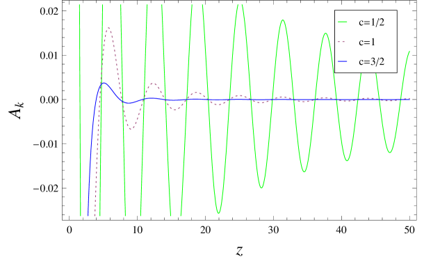
  Figure 2: Figure showing $Re(A)k^{(1-4c)/2}$ as a function of $z(=-k\eta)$ for different $c$. We have also absorbed a factor of $(\gamma H)^{4c}$ into the gauge field for simplicity. The level of damping increases with $c$.

• The second case of interest occurs when $F_{1}(\gamma-q)>>V$, which could arise in the ultra-relativistic regime where $F_{1}\gamma$ is very large. The constraint equation (3.15) then implies that $F_{1}^{2}F_{3}^{2}\sim Z^{2}e^{-4\alpha c_{1}}$, where $c_{1}$ is a dimensionless constant and $Z$ is a dimensionful constant. Since the gauge coupling depends only on $F_{1}F_{3}^{2}$, we must specify one of these two functions completely, before being able to determine the magnetic field spectrum. This new limit is only possible due to the non-linear nature of the DBI action, but appears to depend explicitly on one of the background functions - unlike the previous case. Interestingly this is precisely the combination of parameters that determines the scale of the anisotropies in (3.17). Our emphasis has been on determining $F_{3}$ for a given value of $F_{1}$ unless otherwise stated. Furthermore:

  • Empolying (3.63) induces solutions of the form

    $${\mathsf{A}}(k,\eta)\sim\eta^{(1-Q_{1})/2}\left(A_{1}{\rm J}\left(\frac{Q_{1}-1}{2},k\eta\right)+A_{2}{\rm Y}\left(\frac{Q_{1}-1}{2},k\eta\right)\right),$$ (A.18)

    where $Y$ and $J$ are Bessel functions [31]. The assumption of large $\gamma$ ensures that $Q_{1}$ tends to $4c$ from above for all values of $p>0$. In order to obtain smaller values of $Q_{1}$ we must ensure that $p$ is negative - in particular one can see that the $\gamma$ dependence drops out for $p=-2$ which is plotted in Figure 3, although note that $Q_{1}\to-4$ asymptotically. The solution simplifies in the case of $Q_{1}=1$, which occurs when $p$ takes the critical value $p_{c}$;

    $$p_{c}\sim\frac{\gamma^{2}(2-8c)-6}{(\gamma^{2}-2)(4c-1)},$$ (A.19)

    which asymptotes to $p_{c}=-2$ for large enough $\gamma$ independent of the value of $c$. Therefore, if $Q_{1}$ is constrained to be unity, then we see that $p\to-2$ is an attractor solution. Normalising the solution using the sub-Horizon modes, we can extract the coefficients arising from integration and write the solution:

    $${\mathsf{A}}_{k}\sim e^{-i\pi Q_{1}/4}\sqrt{\frac{\eta^{1-Q_{1}}}{2(-\gamma H)^{Q_{1}}}}H^{(2)}\left(\frac{Q_{1}-1}{2},k\eta\right),$$ (A.20)

    where $H^{(2)}$ is the Hankel function of the second kind, which is illustrated in Figure (3). Note that the attractor solution $p=-2$ ensures that the gauge field is strongly damped. Other values of $p$ tend to lie on the same curves, indicating that the solution is insensitive to the precise form of the power law.

    

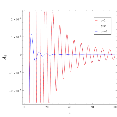
    Figure 3: The real part of the expression $A\sqrt{k^{1-Q}}$ plotted as a function of $z(=-k\eta)$ for $c=1$. We assumed that $H^{2}\sim\gamma/3$ and $\gamma\sim 10$ using Planckian units.

  • From (3.69), we can use it to solve the gauge field energy density constraint to obtain the electromagnetic field as before. The solution is again a Hankel function, but if we solve for the magnetic field we obtain the following scaling

    $$|B_{k}|^{2}\propto H_{I}^{4}H_{I}^{(3-4c)},$$ (A.21)

    which indicates that $c=3/4$ yields a flat spectrum at the end of inflation.

There is also an interesting fixed point solution where we can find $F_{1}F_{3}^{2}=$ constant. In this case we find that a magnetic field emerges during the inflationary phase due to a logarithmic term in the mode expansion of $\mathsf{A}$. Thus the field is driven to be initially large, but decreases rapidly as the universe expands. The gauge field then vanishes identically at the end of inflation - therefore is unable to act as a seed-field to generate the observed magnetic field today.

References

- [1] J. R. Primack, Nucl. Phys. Proc. Suppl. 173 (2007) 1 [arXiv:astro-ph/0609541].
- [2] D. Grasso and H. R. Rubinstein, Phys. Rept. 348, 163 (2001) [arXiv:astro-ph/0009061].
- [3] M. Giovannini, Int. J. Mod. Phys. D 13, 391 (2004) [arXiv:astro-ph/0312614].
- [4] M. S. Turner and L. M. Widrow, Phys. Rev. D 37, 2743 (1988).
- [5] K. Enqvist, Int. J. Mod. Phys. D 7, 331 (1998) [arXiv:astro-ph/9803196].
- [6] C. G. Tsagas, Phys. Rev. D 81, 043501 (2010) [arXiv:0912.2749 [astro-ph.CO]].
- [7] S. Matarrese, S. Mollerach, A. Notari and A. Riotto, Phys. Rev. D 71, 043502 (2005) [arXiv:astro-ph/0410687].
- [8] C. G. Tsagas, P. K. S. Dunsby and M. Marklund, Phys. Lett. B 561, 17 (2003) [arXiv:astro-ph/0112560].
- [9] A. Kandus, K. E. Kunze and C. G. Tsagas, arXiv:1007.3891 [astro-ph.CO].
- [10] K. E. Kunze, Phys. Rev. D 81, 043526 (2010) [arXiv:0911.1101 [astro-ph.CO]].
- [11] A. Dolgov, Phys. Rev. D 48, 2499 (1993) [arXiv:hep-ph/9301280].
- [12] See e.g., P. V. Moniz, Phys. Rev. D 66 (2002) 103501; Phys. Rev. D 66 (2002) 064012; Class. Quant. Grav. 19 (2002) L127. and references therein
- [13] V. V. Dyadichev, D. V. Gal’tsov, A. G. Zorin and M. Y. Zotov, Phys. Rev. D 65 (2002) 084007 [arXiv:hep-th/0111099].
- [14] C. L. Bennett et al., arXiv:1001.4758 [astro-ph.CO].
- [15] K. Land and J. Magueijo, Phys. Rev. Lett. 95, 071301 (2005) [arXiv:astro-ph/0502237].
- [16] C. Copi, D. Huterer, D. Schwarz and G. Starkman, Phys. Rev. D 75, 023507 (2007) [arXiv:astro-ph/0605135].
- [17] T. Kahniashvili, Y. Maravin and A. Kosowsky, Phys. Rev. D 80, 023009 (2009) [arXiv:0806.1876 [astro-ph]].
- [18] S. Kanno, J. Soda and M. a. Watanabe, JCAP 0912, 009 (2009) [arXiv:0908.3509 [astro-ph.CO]].
- [19] A. E. Gumrukcuoglu, B. Himmetoglu and M. Peloso, Phys. Rev. D 81, 063528 (2010) [arXiv:1001.4088 [astro-ph.CO]].
- [20] R. Emami, H. Firouzjahi and M. S. Movahed, Phys. Rev. D 81, 083526 (2010) [arXiv:0908.4161 [hep-th]].
- [21] T. R. Dulaney and M. I. Gresham, Phys. Rev. D 81, 103532 (2010) [arXiv:1001.2301 [astro-ph.CO]].
- [22] M. a. Watanabe, S. Kanno and J. Soda, Phys. Rev. Lett. 102, 191302 (2009) [arXiv:0902.2833 [hep-th]].
- [23] M. a. Watanabe, S. Kanno and J. Soda, arXiv:1003.0056 [astro-ph.CO].
- [24] M. A. Ganjali, JHEP 0509, 004 (2005) [arXiv:hep-th/0509032].
- [25] K. Bamba, N. Ohta and S. Tsujikawa, Phys. Rev. D 78, 043524 (2008) [arXiv:0805.3862 [astro-ph]].
- [26] H. J. Mosquera Cuesta and G. Lambiase, Phys. Rev. D 80, 023013 (2009) [arXiv:0907.3678 [astro-ph.CO]].
- [27] D. N. Vollick, Gen. Rel. Grav. 35, 1511 (2003) [arXiv:hep-th/0102187].
- [28] K. E. Kunze, Phys. Rev. D 77, 023530 (2008) [arXiv:0710.2435 [astro-ph]].
- [29] L. Campanelli, P. Cea, G. L. Fogli and L. Tedesco, Phys. Rev. D 77, 043001 (2008) [arXiv:0710.2993 [astro-ph]].
- [30] L. Campanelli, Phys. Rev. D 80, 063006 (2009) [arXiv:0907.3703 [astro-ph.CO]].
- [31] Table of Integrals, Series, and Products, Sixth Edition, I. S. Gradshteyn, I. M. Ryzhik, A. Jeffrey , D. Zwillinger, Academic Press; 6th edition (August 25, 2000)
- [32] A. R. Liddle, A. Mazumdar and F. E. Schunck, Phys. Rev. D 58, 061301 (1998) [arXiv:astro-ph/9804177].
- [33] P. Kanti and K. A. Olive, Phys. Rev. D 60, 043502 (1999) [arXiv:hep-ph/9903524].
- [34] P. Kanti and K. A. Olive, Phys. Lett. B 464, 192 (1999) [arXiv:hep-ph/9906331].
- [35] E. J. Copeland, A. Mazumdar and N. J. Nunes, Phys. Rev. D 60, 083506 (1999) [arXiv:astro-ph/9904309].
- [36] D. Larson et al., arXiv:1001.4635 [astro-ph.CO].
- [37] L. Leblond and S. Shandera, JCAP 0808, 007 (2008) [arXiv:0802.2290 [hep-th]].
- [38] T. Kobayashi, S. Mukohyama and S. Kinoshita, JCAP 0801, 028 (2008) [arXiv:0708.4285 [hep-th]].
- [39] I. Huston, J. E. Lidsey, S. Thomas and J. Ward, JCAP 0805, 016 (2008) [arXiv:0802.0398 [hep-th]].
- [40] M. Becker, L. Leblond and S. E. Shandera, Phys. Rev. D 76, 123516 (2007) [arXiv:0709.1170 [hep-th]].
- [41] A. Berndsen, J. E. Lidsey and J. Ward, JHEP 1001, 025 (2010) [arXiv:0908.4252 [hep-th]].
- [42] A. Avgoustidis and I. Zavala, JCAP 0901, 045 (2009) [arXiv:0810.5001 [hep-th]].
- [43] F. Bigazzi, A. L. Cotrone, J. Mas, A. Paredes, A. V. Ramallo and J. Tarrio, JHEP 0911, 117 (2009) [arXiv:0909.2865 [hep-th]].
- [44] C. Nunez, A. Paredes and A. V. Ramallo, arXiv:1002.1088 [hep-th].
- [45] A. Sen, JHEP 0204, 048 (2002) [arXiv:hep-th/0203211].
- [46] A. Sen, JHEP 9910, 008 (1999) [arXiv:hep-th/9909062].
- [47] J. Kluson, Phys. Rev. D 62, 126003 (2000) [arXiv:hep-th/0004106].
- [48] M. R. Garousi, Nucl. Phys. B 584, 284 (2000) [arXiv:hep-th/0003122].
- [49] V. Niarchos, arXiv:1005.1650 [hep-th].
- [50] J. Raeymaekers, JHEP 0410, 057 (2004) [arXiv:hep-th/0406195].
- [51] E. Silverstein and D. Tong, Phys. Rev. D 70, 103505 (2004) [arXiv:hep-th/0310221].
- [52] M. Alishahiha, E. Silverstein and D. Tong, Phys. Rev. D 70, 123505 (2004) [arXiv:hep-th/0404084].