Testing metric-affine $f(R)$-gravity by relic scalar gravitational waves

Abstract

We discuss the emergence of scalar gravitational waves in metric-affine $f(R)$-gravity. Such a component allows to discriminate between metric and metric–affine theories The intrinsic meaning of this result is that the geodesic structure of the theory can be discriminated. We extend the formalism of cross correlation analysis, including the additional polarization mode, and calculate the detectable energy density of the spectrum for cosmological relic gravitons. The possible detection of the signal is discussed against sensitivities of VIRGO, LIGO and LISA interferometers.

I Introduction

Extending General Relativity (GR) to more general actions with respect to the Hilbert-Einstein one is revealing a very fruitful approach in modern physics. From a conceptual point of view, there is no a priori reason to restrict the gravitational Lagrangian to a linear function of the Ricci scalar $R$, minimally coupled with matter. The idea that there are no “exact” laws of physics but that the Lagrangians of physical interactions are “stochastic” functions – with the property that local gauge invariances (i.e. conservation laws) are well approximated in the low energy limit and that physical constants can vary – has been recently taken into serious consideration.

Beside fundamental physics motivations, all these theories have acquired a huge interest in cosmology due to the fact that they “naturally” exhibit inflationary behaviors able to overcome the shortcomings of Cosmological Standard Model. Furthermore, dark energy models mainly rely on the implicit assumption that Einstein’s GR is the correct theory of gravity, indeed. Nevertheless, its validity at the larger astrophysical and cosmological scales has never been tested and it is therefore conceivable that both cosmic speed up and missing matter represent signals of a breakdown in our understanding of gravitation law so that one should consider the possibility that the Hilbert - Einstein Lagrangian, linear in the Ricci scalar $R$, should be generalized. Following this line of thinking, the choice of a generic function $f(R)$ can be derived by matching the data and by the ”economic” requirement that no exotic ingredients have to be added. This is the underlying philosophy of what is referred to as $f(R)$–gravity reviews . In this context, the same cosmological constant could be removed as an ingredient of the cosmic pie being nothing else but a particular eigenvalue of a general class of theories garattini .

However $f(R)$–gravity can be encompassed in the Extended Theories of Gravity being a ”minimal” extension of GR where functions of Ricci scalar are taken into account. Although such gravity theories have received much attention in cosmology, since they are naturally able to give rise to accelerating expansions (both in the late and in the early Universe) and systematic studies of the phase space of solutions are in progress cnot , it is possible to demonstrate that $f(R)$–theories can also play a major role at astrophysical scales mnras .

Despite these encouraging results, a major conceptual problem has not been solved indeed: the description of dynamics can be pursued in metric, affine and metric-affine approaches with different results (see reviews for details). This means that the affine connection cannot be simply Levi-Civita, implying that the geodesic and causal structure coincide as in the metric approach, but it could be endowed with a richer geometric structure. For example, if the spacetime is ${\bf U}_{4}$ and not ${\bf V}_{4}$ as in Riemannian geometry, torsion fields have to be considered and connection is not simply Levi-Civita CCSV1 . The consequence of this fact is that geodesic structure and causal structure of spacetime can be disentangled hehl . Probing this feature is a fundamental issue that could have dramatic consequences since further degrees of freedom, like spin or the different types of torsion, should be considered into dynamics CLS . Searching for experimental probes in this direction is a urgent problem faced by several authors (see e.g. guthtor ).

In this paper, we will take into account the metric-affine formulation of $f(R)$-gravity and put in evidence that the difference between a theory à la Palatini and a theory with torsion can be reconducted to the difference between affine connections that results in the relative variation of a scalar field. Such a scalar field is endowed with the further degrees of freedom by which $f(R)$-gravity differs from GR where $f(R)=R$. Assuming that the effect of such a field is a further scalar mode in the relic cosmic background of gravitational waves (GWs), we consider that the possible detection of such a mode could result, for example, as a probe of torsion. On the other hand, the absence of such a component could be a confirmation that the connection is actually Levi-Civita. Besides, detecting new gravitational modes could be a sort of experimentum crucis in order to discriminate among theories since this fact would be the “signature” that GR should be enlarged or modified maggiore ; bellucci ; elizalde . The outline of the paper is as follows. In Sec. II, we give an overview of metric–affine $f(R)$–gravity theories. The linearized theory of gravitational waves is considered in Sec. III . Here, the standard polarization, modes coming from GR, are distinguished with respect to the further possible scalar mode coming from the preceding considerations. In Sect. IV, we investigate the response of a single detector to a GW propagating in certain direction with each polarization mode. Sect. V is devoted to the discussion of the spectrum of the GW stochastic background where the further scalar mode is considered. Conclusions are drawn in Sect. VI.

II Metric-affine $f(R)$-gravity

In metric–affine $f(R)$- gravity, the (gravitational) dynamical fields are pairs $(g,\Gamma)\/$ consisting of a pseudo–Riemannian metric $g\/$ and a linear connection $\Gamma\/$ on the space-time manifold $M\/$. In the Palatini approach, the connection $\Gamma\/$ is torsionless but it is not requested to be metric–compatible, instead, in the approach with torsion, the dynamical connection $\Gamma$ is forced to be metric but it is allowed to have torsion different from zero. The field equations are derived from an action functional of the form

$${\cal A}\/(g,\Gamma)=\int{\left(\sqrt{|g|}f\/(R)+{\cal L}_{m}\right)\,ds}$$ (1)

where $f(R)$ is a real function, $R\/(g,\Gamma)=g^{ij}R_{ij}\/$ (with $R_{ij}:=R^{h}_{\;\;ihj}\/$) is the scalar curvature associated with the connection $\Gamma\/$ and ${\cal L}_{m}\,ds\/$ is a suitable material Lagrangian. Assuming that the material Lagrangian does not depend on the dynamical connection, the field equations are

$$f^{\prime}(R)R_{ij}-\frac{1}{2}f\/(R)g_{ij}=\Sigma_{ij}\,,$$ (2)

$$T_{ij}^{\phantom{ij}h}=-\frac{1}{2f^{\prime}(R)}\frac{\partial{f^{\prime}(R)}}{\partial{x^{p}}}\left(\delta^{p}_{i}\delta^{h}_{j}-\delta^{p}_{j}\delta^{h}_{i}\right)$$ (3)

for $f(R)$-gravity with torsion $T_{ij}^{\phantom{ij}h}\equiv\Gamma^{\phantom{ij}h}_{ij}-\Gamma^{\phantom{ji}h}_{ji}$ CCSV1 ; CCSV2 ; CCSV3 , and

$$f^{\prime}\/(R)R_{ij}-\frac{1}{2}f(R)g_{ij}=\Sigma_{ij}\,,$$ (4)

$$\nabla_{k}(f^{\prime}(R)g_{ij})=0\,,$$ (5)

for $f(R)$-gravity in the Palatini approach francaviglia1 ; Sotiriou ; Sotiriou-Liberati1 ; Olmo . In Eqs. (2) and (4), the quantity ${\displaystyle\Sigma_{ij}:=-\frac{1}{\sqrt{|g|}}\frac{\delta{\cal L}_{m}}{\delta g^{ij}}\/}$ plays the role of stress-energy tensor. Considering the trace of Eqs. (2) and (4), we obtain the relation

$$f^{\prime}\/(R)R-2f\/(R)=\Sigma$$ (6)

linking the curvature scalar $R\/$ with the trace of the stress-energy tensor $\Sigma:=g^{ij}\Sigma_{ij}\/$.

From now on, we shall suppose that the relation (6) is invertible as well as that $\Sigma\neq const$ (this implies, for example, $f(R)\/$ different from $\alpha R^{2}\/$ which is only compatible with $\Sigma=0\/$) . Under these hypotheses, the curvature scalar $R\/$ can be expressed as a suitable function of $\Sigma\/$, namely

$$R=F(\Sigma)\,.$$ (7)

If $\Sigma=const$, GR plus the cosmological constant is recovered CCSV1 . Defining the scalar field

$$\varphi:=f^{\prime}(F(\Sigma))$$ (8)

we can put the Einstein–like field equations of both à la Palatini and with torsion theories in the same form CCSV1 ; Olmo , that is

$$\tilde{R}_{ij}-\frac{1}{2}\tilde{R}g_{ij}=\frac{1}{\varphi}\Sigma_{ij}+\frac{1}{\varphi^{2}}\left(\varphi\tilde{\nabla}_{j}\frac{\partial\varphi}{\partial{x^{i}}}-\frac{3}{2}\frac{\partial\varphi}{\partial{x^{i}}}\frac{\partial\varphi}{\partial{x^{j}}}+\frac{3}{4}\frac{\partial\varphi}{\partial{x^{h}}}\frac{\partial\varphi}{\partial{x^{k}}}g^{hk}g_{ij}-\varphi\tilde{\nabla}^{h}\frac{\partial\varphi}{\partial{x^{h}}}g_{ij}-V\/(\varphi)g_{ij}\right)\,,$$

where we have introduced the effective potential

$$V\/(\varphi):=\frac{1}{4}\left[\varphi F^{-1}\/((f^{\prime})^{-1}\/(\varphi))+\varphi^{2}\/(f^{\prime})^{-1}\/(\varphi)\right]\,,$$ (10)

for the scalar field $\varphi\/$. In Eq. (II), $\tilde{R}_{ij}\/$, $\tilde{R}\/$ and $\tilde{\nabla}\/$ denote respectively the Ricci tensor, the scalar curvature and the covariant derivative associated with the Levi–Civita connection of the dynamical metric $g_{ij}$. Therefore, if the dynamical connection $\Gamma\/$ is not coupled with matter, both the theories (with torsion and Palatini–like) generate identical Einstein–like field equations.

On the contrary, the field equations for dynamical connection are different and (in general) give rise to different solutions. In fact, the connection $\Gamma$ solution of Eqs. (3) is

$$\Gamma_{ij}^{\phantom{ij}h}=\tilde{\Gamma}_{ij}^{\phantom{ij}h}+\frac{1}{2\varphi}\frac{\partial\varphi}{\partial{x^{j}}}\delta^{h}_{i}-\frac{1}{2\varphi}\frac{\partial\varphi}{\partial{x^{p}}}g^{ph}g_{ij}$$ (11)

where $\tilde{\Gamma}_{ij}^{\phantom{ij}h}\/$ denote the coefficients of the Levi–Civita connection associated with the metric $g_{ij}$, while the connection $\bar{\Gamma}\/$ solution of Eqs. (5) is

$$\bar{\Gamma}_{ij}^{\phantom{ij}h}=\tilde{\Gamma}_{ij}^{\phantom{ij}h}+\frac{1}{2\varphi}\frac{\partial\varphi}{\partial{x^{j}}}\delta^{h}_{i}-\frac{1}{2\varphi}\frac{\partial\varphi}{\partial{x^{p}}}g^{ph}g_{ij}+\frac{1}{2\varphi}\frac{\partial\varphi}{\partial{x^{i}}}\delta^{h}_{j}\,,$$ (12)

and coincides with the Levi–Civita connection induced by the conformal metric $\bar{g}_{ij}:=\varphi g_{ij}$. By comparison, the connections $\Gamma$ and $\bar{\Gamma}$ satisfy the relation

$$\bar{\Gamma}_{ij}^{\phantom{ij}h}-\Gamma_{ij}^{\phantom{ij}h}=\frac{1}{2\varphi}\frac{\partial\varphi}{\partial{x^{i}}}\delta^{h}_{j}\,.$$ (13)

Of course, the Einstein–like equations (II) are coupled with the matter field equations. In this respect, it is worth pointing out that Eqs. (II) imply the same conservation laws holding in GR CV1 ; CV2 ; CV3 . An important consideration is in order at this point. The difference between the affine connections in theories with torsion and à la Palatini is characterized by the relative variation of the scalar field $\varphi$, which is determined by the matter-energy $\Sigma$. Assuming such a difference as a perturbation in a fixed conformal background, we can investigate if a scalar mode of gravitational radiation could be related with it. This will be the argument of the next section.

III The scalar mode of gravitational waves and polarization states

The geodesic structure of metric-affine $f(R)$-gravity could be tested by detecting a further polarization in gravitational radiation related to a scalar mode. To be more precise, the scalar field is a way to define the further gravitational degrees of freedom emerging from $f(R)$-gravity. The total GW has to be a function of the standard modes coming from GR and modes coming from these further degrees of freedom, that is $h^{(tot)}_{ij}=h^{(tot)}_{ij}(h_{ij},h_{\varphi})$. The following derivation will show this statement.

Let us consider a small perturbation on a conformal background characterized by a Minkowskian spacetime on which a scalar field $\varphi=\varphi_{0}$ is defined. Perturbing the background at first order, we obtain

$$\begin{array}[]{c}\tilde{g}_{ij}=\eta_{ij}+h_{ij}\,,\qquad\varphi=\varphi_{0}+\delta\varphi.\end{array}$$ (14)

From these linearized quantities, it is possible to derive the related curvature invariants $\widetilde{R}_{ijkl}$, $\widetilde{R}_{ij}$ and $\widetilde{R}$ and the field equations:

$$\begin{array}[]{c}\widetilde{R}_{ij}-\frac{\widetilde{R}}{2}\eta_{ij}=(\partial_{i}\partial_{j}h_{\varphi}-\eta_{ij}\square h_{\varphi})\,,\qquad{}\square h_{\varphi}=m^{2}h_{\varphi},\end{array}$$ (15)

where $\displaystyle{h_{\varphi}\equiv\frac{\delta\varphi}{\varphi_{0}}}$ (see CST for details). On the other hand, such equations can be obtained directly starting from the field Eqs.(II) with the potential (10). It is straightforward to see that $\displaystyle{\delta\varphi=\frac{\partial\varphi}{\partial x^{i}}\delta x^{i}}$ being $\delta x^{i}=dx^{i}$. Looking at Eq. (13), it is clear that the relative variation of the scalar field with respect to the background gives the difference between the connections $\bar{\Gamma}$ and $\Gamma$ and then it is the signature of the fact that connection is not Levi-Civita. Besides, being the Klein-Gordon equation for the scalar field $\varphi$ in Minkowski spacetime

$$\square\varphi=\frac{dV}{d\varphi}\,,$$ (16)

and perturbing Eq.(10), we have at the lowest order

$$V\simeq\frac{1}{2}m^{2}\,\delta\varphi^{2}\Rightarrow\frac{dV}{d\varphi}\simeq m^{2}\delta\varphi,$$ (17)

and then the above result in (15). The constant $m$ has the dimensions of a mass. $\widetilde{R}_{ijkl}$ and Eqs. (15) are invariants for gauge transformations maggiore

$$\begin{array}[]{c}h_{ij}\rightarrow h^{\prime}_{ij}=h_{ij}-\partial_{(i}\epsilon_{j)}\,,\qquad\delta\varphi\rightarrow\delta\varphi^{\prime}=\delta\varphi;\end{array}$$ (18)

then

$$\bar{h}_{ij}\equiv h_{ij}-\frac{h}{2}\eta_{ij}$$ (19)

can be defined. Here $h$ is the trace. By considering suitable transformation parameters $\epsilon^{j}$, one gets an equivalent Lorentz gauge where the following equations hold

$$\partial^{i}\bar{h}_{ij}=0\,.$$ (20)

According to this choice, field equations read

$$\square\bar{h}_{ij}=0\,,\qquad\square h_{\varphi}=m^{2}h_{\varphi}\,.$$ (21)

Solutions of Eqs.(21) are plane waves:

$$\bar{h}_{ij}=A_{ij}(\overrightarrow{k})\exp(ik^{j}x_{j})+c.c.\,,$$ (22)

$$h_{\varphi}=a(\overrightarrow{k})\exp(iq^{j}x_{j})+c.c.\,,$$ (23)

where the following dispersion relations hold

$$\begin{array}[]{ccc}k^{j}\equiv(\omega,\overrightarrow{k})\,,&&\omega=k\equiv|\overrightarrow{k}|\,,\\ \\ q^{j}\equiv(\omega_{m},\overrightarrow{k})\,,&&\omega_{m}=\sqrt{m^{2}+k^{2}}.\end{array}$$ (24)

The polarization tensor $A_{ij}(\overrightarrow{k})$ can be found following the arguments in Ref. vanDam:1970vg ; greci . Here Eq. (22) represents the standard waves of GR Misner ; Allen . Eq. (23) is the solution for the massive mode. The fact that the dispersion law for the modes of the massive field $h_{\varphi}$ is not linear has to be stressed. The velocity of every “ordinary” mode $\bar{h}_{ij}$, arising from GR, is the light speed $c$, but the dispersion law (the second of Eq. (24)) for the modes of $h_{\varphi}$ is that of a massive field. It can be discussed as a wave-packet propagating on the background. Also, the group-velocity of a wave-packet of $h_{\varphi}$ centered in $\overrightarrow{k}$ is

$$\overrightarrow{v_{G}}=\frac{\overrightarrow{k}}{\omega_{m}},$$ (25)

which is exactly the velocity of a massive particle with mass $m$, momentum $\overrightarrow{k}$ and frequency $f=\omega_{m}/2\pi$. From the second of Eqs. (24) and Eq. (25), it is straightforward to obtain:

$$v_{G}=\frac{\sqrt{\omega_{m}^{2}-m^{2}}}{\omega_{m}}.$$ (26)

Then, assuming a constant speed for the wave-packet, it has to be

$$m=\sqrt{(1-v_{G}^{2})}\omega_{m}.$$ (27)

Now, it has to be discussed if there could be phenomenological limitations to the GW-mass. A strong limitation arises from the fact that the GW should be in a frequency which falls in the frequency-range for both Earth-based and space-based gravitational antennas, that is the interval $10^{-4}Hz\leq f\leq 10KHz$ acernese ; willke ; sigg ; abbott ; ando ; tatsumi ; lisa1 ; lisa2 . For a massive GW, it is:

$$2\pi f=\omega_{m}=\sqrt{m^{2}+k^{2}}\,.$$ (28)

Thus, it has to be

$$0\leq m\leq 10^{-11}eV.$$ (29)

A stronger limitation is given by the requirements coming from cosmology and Solar System tests on modified theories of gravity (see e.g. maggiore ). In this case, it is

$$0\leq m\leq 10^{-33}eV.$$ (30)

These scalar GW modes can be dealt as very light particles.

Let us consider now the GW- polarization states. The above gauge gives $k^{i}A_{ij}=0$. Moreover, we assume that $\overrightarrow{k}$ is in the $z$ direction and we choose a gauge in which only $A_{11}=-A_{22}$, and $A_{12}=A_{21}$ are different from zero. In this frame, we take a polarization base of the form

$$e_{ij}^{(+)}=\frac{1}{\sqrt{2}}\left(\begin{array}[]{cccc}0&0&0&0\\ 0&1&0&0\\ 0&0&-1&0\\ 0&0&0&0\end{array}\right),\qquad e_{ij}^{(\times)}=\frac{1}{\sqrt{2}}\left(\begin{array}[]{cccc}0&0&0&0\\ 0&0&1&0\\ 0&1&0&0\\ 0&0&0&0\end{array}\right)\,,\qquad e_{ij}^{(s)}=\frac{1}{\sqrt{2}}\left(\begin{array}[]{cccc}0&0&0&0\\ 0&0&0&0\\ 0&0&0&0\\ 0&0&0&1\end{array}\right).$$ (31)

The resulting GW is

$$h^{(tot)}_{ij}(t,z)=A^{+}(t-z)e_{ij}^{(+)}+A^{\times}(t-z)e_{ij}^{(\times)}+h_{\varphi}(t-v_{G}z)e_{ij}^{s}.$$ (32)

The first two terms $A^{+}(t-z)e_{ij}^{(+)}$ and $A^{\times}(t-z)e_{ij}^{(\times)}$ describe the two standard polarizations of gravitational waves that arise from GR, while the term $h_{\varphi}(t-v_{G}z)e_{ij}^{s}$ is the massive field arising from $f(R)$-gravity. According to the derivation of previous section, it could characterize the fact that connection is not Levi-Civita and then the geodesic structure of the theory could be distinguishable with respect to the causal structure. In Fig.1, we illustrate how each GW polarization affects test masses arranged on a circle.

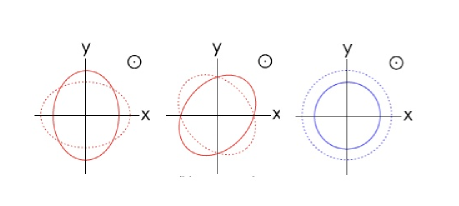
Figure 1: The polarization modes of gravitational waves. In the figure, displacements that each mode induces on a sphere of test particles are shown. We have respectively the standard plus and cross modes of GR, and the scalar mode related to the scalar field. The circled dots represent the inward propagating direction, orthogonal to the plane.

IV The response of interferometers to scalar gravitational waves

Let us compute now the response measured in an interferometer when a GW is coming from an arbitrary direction. We suppose that a further polarization, related to the scalar mode, is present so the antenna pattern should say, in principle, if the detection of such a mode is possible. First of all, let us construct a response tensor or detector tensor $\mathbf{D}$ such that the signal induced in the detector by a GW of polarization $\mathbf{e}$ is proportional to the angular pattern function of a detector. It is

$$F_{pattern}(\hat{\mathbf{\Omega}})=\mathbf{D}:\mathbf{e}_{pattern}(\hat{\mathbf{\Omega}})\,,\qquad\mathbf{D}=\frac{1}{2}\left[\hat{\mathbf{u}}\otimes\hat{\mathbf{u}}-\hat{\mathbf{v}}\otimes\hat{\mathbf{v}}\right]\>,$$ (33)

here we have $pattern=+,\times,s$. The symbol ”:” is the contraction between tensors. $\mathbf{D}$ maps the metric perturbation in a signal on the detector. The vectors $\hat{\mathbf{u}}$ and $\hat{\mathbf{v}}$ are unitary and orthogonal to each other. They are directed to each detector arm and form an orthonormal system with the unitary vector $\hat{\mathbf{w}}$. $\hat{\mathbf{\Omega}}$ is the unitary vector directed along the GW propagation; $\hat{\mathbf{m}}$ and $\hat{\mathbf{n}}$ are two orthonormal vectors (see Fig. 2). Eq. (33) holds only when the arm length of the detector is smaller and smaller than the GW wavelength that we are taking into account. This is relevant to deal with ground-based laser interferometers but this condition could not be valid when dealing with space interferometers like LISA. However, more accurate studies have to be pursued on this issue.

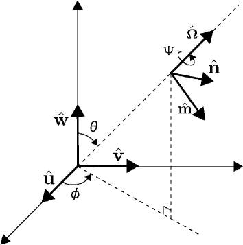
Figure 2: The coordinate systems used to calculate the polarization tensors and the pictorial view of the coordinate transformation.

A standard orthonormal coordinate system for the detector is

$$\left\{\begin{array}[]{lll}\hat{\mathbf{u}}=(1,0,0)\\ \hat{\mathbf{v}}=(0,1,0)\\ \hat{\mathbf{w}}=(0,0,1)\,.\end{array}\right.\;$$ (34)

On the other hand, the coordinate system for the GW, rotated by angles $(\theta,\phi)$, is given by

$$\left\{\begin{array}[]{lll}\displaystyle\hat{\mathbf{u}}^{\prime}=(\cos\theta\cos\phi,\cos\theta\sin\phi,-\sin\theta)\\ \displaystyle\hat{\mathbf{v}}^{\prime}=(-\sin\phi,\cos\phi,0)\\ \displaystyle\hat{\mathbf{w}}^{\prime}=(\sin\theta\cos\phi,\sin\theta\sin\phi,\cos\theta)\end{array}\right.\;.$$ (35)

The rotation with respect to the angle $\psi$, around the GW-propagating axis, gives the most general choice for the coordinate system, that is

$$\left\{\begin{array}[]{lll}\displaystyle\hat{\mathbf{m}}=\hat{\mathbf{u}}^{\prime}\cos\psi+\hat{\mathbf{v}}^{\prime}\sin\psi\\ \displaystyle\hat{\mathbf{n}}=-\hat{\mathbf{v}}^{\prime}\sin\psi+\hat{\mathbf{u}}^{\prime}\cos\psi\\ \displaystyle\hat{\mathbf{\Omega}}=\hat{\mathbf{w}}^{\prime}\end{array}\right.\;.$$ (36)

Coordinates $(\hat{\mathbf{u}},\hat{\mathbf{v}},\hat{\mathbf{w}})$ are related to the coordinates $(\hat{\mathbf{m}},\hat{\mathbf{n}},\hat{\mathbf{\Omega}})$ by the rotation angles ($\phi,\,\theta,\,\psi$)as indicated in Fig.2. From the vectors $\hat{\mathbf{m}}$, $\hat{\mathbf{n}}$, and $\hat{\mathbf{\Omega}}$, the polarization tensors are

$$\mathbf{e}_{+} = \frac{1}{\sqrt{2}}\left(\hat{\mathbf{m}}\otimes\hat{\mathbf{m}}-\hat{\mathbf{n}}\otimes\hat{\mathbf{n}}\right)\;,$$ (37)

$$\mathbf{e}_{\times} = \frac{1}{\sqrt{2}}\left(\hat{\mathbf{m}}\otimes\hat{\mathbf{n}}+\hat{\mathbf{n}}\otimes\hat{\mathbf{m}}\right)\;,$$ (38)

$$\mathbf{e}_{s} = \frac{1}{\sqrt{2}}\left(\hat{\mathbf{\Omega}}\otimes\hat{\mathbf{\Omega}}\right)\;.$$ (39)

Taking into account Eqs. (33), the angular patterns for each polarization are

$$F_{+}(\theta,\phi,\psi) = \frac{1}{\sqrt{2}}(1+\cos^{2}\theta)\cos 2\phi\cos 2\psi-\cos\theta\sin 2\phi\sin 2\psi\;,$$ (40)

$$F_{\times}(\theta,\phi,\psi) = -\frac{1}{\sqrt{2}}(1+\cos^{2}\theta)\cos 2\phi\sin 2\psi-\cos\theta\sin 2\phi\cos 2\psi\;,$$ (41)

$$F_{s}(\theta,\phi) = \frac{1}{\sqrt{2}}\sin^{2}\theta\cos 2\phi\;.$$ (42)

The angular pattern functions for each polarization are plotted in Figs. 3 and 4. The figures show the sensitivity (i.e. the ”gain”) of the interferometer in a given direction. A typical antenna pattern presents some maxima of sensitivity (lobes); the strongest of these maxima (the main lobe) defines the direction in which the antenna is most sensitive maggiore . These considerations indicate that the signal related to the scalar component (42) is, in principle, detectable. Our results are consistent, for example, with those in abio ; nishi ; tobar . Another possibility to investigate the presence of GW-scalar components is to consider the stochastic background of GWs as we will do in the next section.

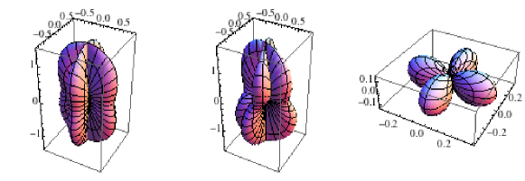
Figure 3: The angular pattern (i.e. the sensitivity) of interferometer for $+$, $\times$ and scalar polarizations.

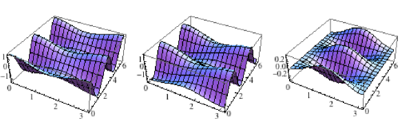
Figure 4: The propagation effects of $+$, $\times$ and scalar polarizations.

V GW-scalar component in the stochastic background

The primordial physical process can give rise to the characteristic spectrum $\Omega_{\varphi}$ for the early stochastic background of relic scalar GWs. The production processes have been analyzed, for example, in Allen ; Grishchuk but only for the tensorial components related to the standard GR. Actually the process can be improved considering also the scalar-tensor component considered here.

Before starting with the analysis, it has to be stressed that the stochastic background of scalar GWs related to the scalar field $\varphi$ can be characterized by a dimensionless spectrum (see the analogous definition for tensorial waves in maggiore ; Allen ; Grishchuk ; AO )

$$\Omega_{\varphi}(f)=\frac{1}{\rho_{c}}\frac{d\rho_{\varphi}}{d\ln f},$$ (43)

where

$$\rho_{c}\equiv\frac{3H_{0}^{2}}{8\pi G}$$ (44)

is the today critical energy density of the Universe, $H_{0}$ the today observed Hubble expansion rate, and $d\rho_{\varphi}$ is the energy density of the scalar part of the gravitational radiation contained in the frequency range $f$ to $f+df$. We are considering now standard units.

The existence of a relic stochastic background of scalar GWs is a consequence of general assumptions. Essentially it derives from basic principles of Quantum Field Theory and GR. The strong variations of gravitational field in the early Universe amplifies the zero-point quantum fluctuations and produces relic GWs. It is well known that the detection of relic GWs is the only way to learn about the evolution of the very early Universe, up to the bounds of the Planck epoch and the initial singularity maggiore ; Allen ; Grishchuk . It is very important to stress the unavoidable and fundamental character of such a mechanism. It directly derives from the inflationary scenario Watson ; Guth , which well fit the WMAP data that are in particular good agreement with almost exponential inflation and spectral index $\approx 1$ peacock .

A remarkable fact about the inflationary scenario is that it contains a natural mechanism which gives rise to perturbations for any field. It is important for our aims that such a mechanism provides also a distinctive spectrum for relic scalar GWs. These perturbations, in inflationary cosmology, arise from the most basic quantum mechanical effect: the uncertainty principle. In this way, the spectrum of relic GWs that we could detect today is nothing else but the adiabatically-amplified zero-point fluctuations Allen ; Grishchuk . The calculation for a simple inflationary model can be performed for the scalar field component. Let us assume that the early Universe is described by an inflationary de Sitter phase emerging in a radiation dominated phase Allen ; Grishchuk ; AO . The conformal metric element is

$$ds^{2}=a^{2}(\eta)[-d\eta^{2}+d\overrightarrow{x}^{2}+h^{(tot)}_{ij}(\eta,\overrightarrow{x})dx^{i}dx^{j}],$$ (45)

where, for a purely scalar GW the metric perturbation (32) reduces to

$$h^{(tot)}_{ij}=h_{\varphi}e_{ij}^{(s)}.$$ (46)

Let us assume a phase transition between a de Sitter and a radiation-dominated phase Allen ; Grishchuk , we have: $\eta_{1}$ is the inflation-radiation transition conformal time and $\eta_{0}$ is the value of conformal time today. If we express the scale factor in terms of comoving time $cdt=a(t)d\eta$, we have

$$a(t)\propto\exp(H_{ds}t),\qquad a(t)\propto\sqrt{t}$$ (47)

for the de Sitter and radiation phases respectively. In order to solve the horizon and flatness problems, the condition ${\displaystyle\frac{a(\eta_{0})}{a(\eta_{1})}>10^{27}}$ has to be satisfied. The relic scalar-tensor GWs are the weak perturbations $h^{(tot)}_{ij}(\eta,\overrightarrow{x})$ of the metric (46) which can be written in the form

$$h^{(tot)}_{ij}=e_{ij}^{(s)}(\hat{k})X(\eta)\exp(i\overrightarrow{k}\cdot\overrightarrow{x}),$$ (48)

in terms of the conformal time $\eta$ where $\overrightarrow{k}$ is a constant wave-vector. From Eqs. (23) and (48), the scalar component is

$$h_{\varphi}(\eta,\overrightarrow{k},\overrightarrow{x})=X(\eta)\exp(i\overrightarrow{k}\cdot\overrightarrow{x}),$$ (49)

where we have specified the amplitude and the phase to the cosmological case. Assuming $Y(\eta)=a(\eta)X(\eta)$, from the Klein-Gordon equation in the FRW metric, one gets

$$Y^{\prime\prime}+(|k|^{2}-\frac{a^{\prime\prime}}{a})Y=0$$ (50)

where the prime denotes the derivative with respect to the conformal time. The solutions of Eq. (50) can be expressed in terms of Hankel functions in both the inflationary and radiation dominated eras, that is:
for $\eta<\eta_{1}$

$$X(\eta)=\frac{a(\eta_{1})}{a(\eta)}[1+H_{ds}\omega^{-1}]\exp(-ik(\eta-\eta_{1})),$$ (51)

for $\eta>\eta_{1}$

$$X(\eta)=\frac{a(\eta_{1})}{a(\eta)}\left[\alpha\exp(-ik(\eta-\eta_{1}))+\beta\exp ik(\eta-\eta_{1})\right],$$ (52)

where $\omega=ck/a$ is the angular frequency of the wave (which is a function of time only being $k=|\overrightarrow{k}|$ constant); $\alpha$ and $\beta$ are time-independent constants which we can obtain demanding that both $X$ and $dX/d\eta$ are continuous at the boundary $\eta=\eta_{1}$ between the inflationary and the radiation dominated eras. By this constraint, we obtain

$$\alpha=1+i\frac{\sqrt{H_{ds}H_{0}}}{\omega}-\frac{H_{ds}H_{0}}{2\omega^{2}}\,,\qquad\beta=\frac{H_{ds}H_{0}}{2\omega^{2}}$$ (53)

In Eqs. (53), $\omega=ck/a(\eta_{0})$ is the angular frequency as observed today, $H_{0}=c/\eta_{0}$ is the Hubble expansion rate as observed today. Such calculations are referred in literature as the Bogoliubov coefficient methods Allen ; Grishchuk .

In an inflationary scenario, every classical or macroscopic perturbation is damped out by the inflation, i.e. the minimum allowed level of fluctuations is that required by the uncertainty principle. Solution (51) corresponds to a de Sitter vacuum state. If the period of inflation is long enough, the today observable properties of the Universe should be indistinguishable from the properties of a Universe started in the de Sitter vacuum state. In the radiation dominated phase, the eigenmodes which describe particles are the coefficients of $\alpha$ while $\beta$- coefficients describe antiparticles (see also tuning ). Thus, the number of particles created at angular frequency $\omega$ in the radiation dominated phase is

$$N_{\omega}=|\beta_{\omega}|^{2}=\left(\frac{H_{ds}H_{0}}{2\omega^{2}}\right)^{2}.$$ (54)

Furthermore, it is possible to write an expression for the energy density of the stochastic background of scalar relic gravitons in the frequency interval $(\omega,\omega+d\omega)$ as

$$d\rho_{\varphi}=2\hbar\omega\left(\frac{\omega^{2}d\omega}{2\pi^{2}c^{3}}\right)N_{\omega}=\frac{\hbar H_{ds}^{2}H_{0}^{2}}{4\pi^{2}c^{3}}\frac{d\omega}{\omega}=\frac{\hbar H_{ds}^{2}H_{0}^{2}}{4\pi^{2}c^{3}}\frac{df}{f}\,,$$ (55)

where $f$, as above, is the frequency in standard comoving time. Eq. (55) can be rewritten in terms of the today and de Sitter value of energy density being

$$H_{0}=\frac{8\pi G\rho_{c}}{3c^{2}}\,,\qquad H_{ds}=\frac{8\pi G\rho_{ds}}{3c^{2}}.$$ (56)

Introducing the Planck density ${\displaystyle\rho_{Planck}=\frac{c^{7}}{\hbar G^{2}}}$, the spectrum is given by

$$\Omega_{\varphi}(f)=\frac{1}{\rho_{c}}\frac{d\rho_{\varphi}}{d\ln f}=\frac{f}{\rho_{c}}\frac{d\rho_{\varphi}}{df}=\frac{16}{9}\frac{\rho_{ds}}{\rho_{Planck}}.$$ (57)

At this point, some comments are in order. First of all, such a calculation works for a simplified model that does not include the matter dominated era. If such an era is also included, the redshift at equivalence epoch has to be considered. Taking into account results in Allen , we get

$$\Omega_{\varphi}(f)=\frac{16}{9}\frac{\rho_{ds}}{\rho_{Planck}}(1+z_{eq})^{-1},$$ (58)

for the waves which, at the epoch in which the Universe becomes matter dominated, have a frequency higher than $H_{eq}$, the Hubble parameter at equivalence. This situation corresponds to frequencies $f>(1+z_{eq})^{1/2}H_{0}$. The redshift correction in Eq.(58) is needed since the today observed Hubble parameter $H_{0}$ would result different without a matter dominated contribution. At lower frequencies, the spectrum is given by Allen ; Grishchuk

$$\Omega_{\varphi}(f)\propto f^{-2}.$$ (59)

As a further consideration, let us note that the results in Eqs. (57) and (58), which are not frequency dependent, do not work correctly in all the range of physical frequencies. For waves with frequencies less than today observed $H_{0}$, the notion of energy density has no sense since the wavelength becomes longer than the Hubble scale of the Universe. In analogous way, at high frequencies, there is a maximal frequency above which the spectrum rapidly drops to zero. In the above calculation, the simple assumption that the phase transition from the inflationary to the radiation dominated epoch is instantaneous has been made. In the physical Universe, this process occurs over some time scale $\Delta\tau$, being

$$f_{max}=\frac{a(t_{1})}{a(t_{0})}\frac{1}{\Delta\tau},$$ (60)

which is the redshifted rate of the transition. In any case, $\Omega_{\varphi}$ drops rapidly. The two cutoffs at low and high frequencies for the spectrum guarantee that the total energy density of the relic scalar gravitons is finite. For Grand Unified Theories energy-scale inflation, it is of the order Allen

$$\frac{\rho_{ds}}{\rho_{Planck}}\approx 10^{-12}.$$ (61)

These results can be quantitatively constrained considering the WMAP release. In fact, it is well known that WMAP observations put severe restrictions on the spectrum. Considering the ratio $\rho_{ds}/\rho_{Planck}$, the relic scalar GW spectrum seems consistent with the WMAP constraints on scalar perturbations. Nevertheless, since the spectrum falls off $\propto f^{-2}$ at low frequencies, this means that today, at LIGO-VIRGO and LISA frequencies, one gets

$$\Omega_{\varphi}(f)h_{100}^{2}<2.3\times 10^{-12}.$$ (62)

It is interesting to calculate the corresponding strain at $\approx 100Hz$, where interferometers like VIRGO and LIGO reach a maximum in sensitivity. The well known equation for the characteristic amplitude Allen ; Grishchuk adapted to the scalar component of GWs can be used:

$$h_{\varphi}(f)\simeq 1.26\times 10^{-18}(\frac{1Hz}{f})\sqrt{h_{100}^{2}\Omega_{\varphi}(f)},$$ (63)

and then we obtain

$$h_{\varphi}(100Hz)<2\times 10^{-26}.$$ (64)

Then, since we expect a sensitivity of the order of $10^{-22}$ for the above interferometers at $\approx 100Hz$, we need to gain four order of magnitude. Let us analyze the situation also at smaller frequencies. The sensitivity of the VIRGO interferometer is of the order of $10^{-21}$ at $\approx 10Hz$ and in that case it is

$$h_{\varphi}(100Hz)<2\times 10^{-25}.$$ (65)

The sensitivity of the LISA interferometer will be of the order of $10^{-22}$ at $\approx 10^{-3}Hz$ and in that case it is

$$h_{\varphi}(100Hz)<2\times 10^{-21}.$$ (66)

This means that a stochastic background of relic scalar GWs could be, in principle, detected by the LISA interferometer.

VI Discussion and conclusions

In this paper, we have investigated the possibility that metric-affine $f(R)$ theories could be distinguished from purely metric ones, by considering the difference in affine connections which result in the relative variation of a suitable scalar field. The absence of such a variation, that is ${\displaystyle\frac{\delta\varphi}{\varphi}=0}$, is the indication that the connection is Levi-Civita. In other words, geodesic structure and causal structure of the theory coincide. On the other hand, if ${\displaystyle\frac{\delta\varphi}{\varphi}\neq 0}$ a more general theory, formulated onto a ${\bf U}_{4}$ manifold, has to be considered. In principle, such an issue could be tested at a fundamental level by detecting possible scalar modes of GWs. This is the key point of this paper.

In this perspective, we have investigated the detectability of additional polarization modes of a stochastic GW background by ground-based laser-interferometric detectors and space-interferometers. Such polarization modes, in general, appear in the extended theories of gravitation and can be utilized to constrain the theories beyond GR in a model-independent way. However, a point has to be discussed in detail. If the interferometer is directionally sensitive and we also know the orientation of the source (and of course if the source is coherent) the situation is straightforward. In this case, the massive mode coming from $f(R)$-gravity would induce longitudinal displacements along the direction of propagation which should be detectable and only the amplitude due to the scalar mode would be the true, detectable, ”new” signal greci . On the other hand, in the case of the stochastic background, there is no coherent source and no directional detection of the gravitational radiation. What the interferometer picks is just an averaged signal coming from the contributions of all possible modes from (uncorrelated) sources all over the celestial sphere. Since we expect the background to be isotropic, the signal will be the same regardless of the orientation of the interferometer, no matter how or on which plane it is rotated, it would always record the characteristic amplitude $h_{\varphi}$. So there is intrinsically no way to disentangle any of the mode in the background, being $h_{\varphi}$ related to the total energy density of the gravitational radiation, which depends on the number of modes available.

This is the why we have considered only $h_{\varphi}$ in the above cross-correlation analysis without giving further fine details coming from polarization. For the situation considered here, we have found that the massive modes are certainly of interest for direct attempts of detection by the LISA experiment. It is, in principle, possible that massive GW modes could be produced in more significant quantities in cosmological or early astrophysical processes in alternative theories of gravity. This situation should be kept in mind when looking for a signature distinguishing these theories from GR, and seems to deserve further investigation. From our point of view, it is of extremely importance since it could allow to distinguish the same structure of the space-time.

However, some further considerations are necessary at this point. According to CNO , $f(R)$-gravity in metric formalism can be presented as an effective dark fluid assuming both the role of dark energy and dark matter. Evidently, metric-affine $f(R)$-gravity may be also presented as (different) effective dark fluid. The above results could contribute in discriminating between the two approaches, if the signature of affine connections is experimentally selected. In particular, torsion could have a relevant role in structure formation and in coincidence problem between dark energy and dark matter as discussed in CCSV1 ; CCSV2 . In this sense, dynamics is richer than that presented in CNO . Furthermore, it is well known that not all metric $f(R)$-gravity model may pass local tests, like Brans-Dicke test, Newton law, etc . The aim is to find out self-consistent models matching Solar System scales with extragalactic and cosmological scales. In NO1 ; NO2 , criteria and several explicit models which pass local tests are given. In this paper, we have not faced this problem since we are using general $f(R)$-gravity models with the only request that they are analytic and Taylor expandable. These are sufficient conditions to discuss scalar GWs. In order to construct a reliable theory, also the problem of background has to be considered together with the stochastic GWs. This will be the argument of forthcoming researches aimed to achieve comprehensive and self-consistent models.

References

-
(1)
S. Nojiri, S. D. Odintsov Int. J. Geom. Meth. Mod. Phys.
4,115
(2007).
S. Capozziello, M. Francaviglia, Gen. Rel. Grav. 40, 357 (2008);
S. Capozziello, M. De Laurentis, V. Faraoni, The Open Astronomy Journal 2, 1874, (2009);
T. P. Sotiriou, V. Faraoni, Rev. Mod. Phys. 82, 451 (2010);
A. De Felice, S. Tsujikawa, arXiv: 1002.4928 [gr-qc] (2010). - (2) S. Capozziello, R. Garattini, Class. Quant. Grav. 24, 1627 (2007).
- (3) S. Capozziello, S. Nojiri, S.D. Odintsov, A. Troisi. Phys. Lett. 639 B, 135 (2006).
-
(4)
S. Capozziello, E. De Filippis, V. Salzano, Mon. Not. Roy. Soc. 394, 947 (2009);
R. Reyes et al., Nature, 464, 256 (2010). - (5) S. Capozziello, R. Cianci, C. Stornaiolo and S. Vignolo, Class. Quantum Grav., 24, 6417 (2007).
- (6) F.W. Hehl, P. von der Heyde, G. D Kerlick and J.M. Nester, Rev. Mod. Phys. 48, 393 (1976).
- (7) S. Capozziello, G. Lambiase, C. Stornaiolo, Annals Phys. (Leipzig) 10, 713 (2001).
- (8) Y. Mao, M. Tegmark, A. Guth, S. Cabi, Phys. Rev. D 76, 104029 (2007).
- (9) M. Maggiore, Phys. Rep. 331, 283 (2000).
- (10) S. Bellucci, S. Capozziello, M. De Laurentis, V. Faraoni, Phys. Rev. D 79, 104004 (2009).
- (11) S. Capozziello, E. Elizalde, S. Nojiri, S. D. Odintsov. Phys. Lett. B 671, 193 (2009).
- (12) S. Capozziello, R. Cianci, C. Stornaiolo and S. Vignolo, Phys.Scripta, 78, 065010 (2008).
- (13) S. Capozziello, R. Cianci, C. Stornaiolo and S. Vignolo, Int.J.Geom.Meth.Mod.Phys , 5, 765 (2008).
- (14) G. Magnano, M. Ferraris and M. Francaviglia, Gen. Rel. Grav. 19, 465 (1987).
- (15) T. P. Sotiriou, Class. Quantum Grav., 23, 1253, (2006).
- (16) T. P. Sotiriou and S. Liberati, Ann. Phys., 322, 935, (2006).
- (17) G. J. Olmo, Phys. Rev. D, 72, 083505, (2005).
- (18) S. Capozziello and S. Vignolo, Class. Quantum Grav., 26, 175013, (2009).
- (19) S. Capozziello and S. Vignolo, Class. Quantum Grav., 26, 168001, (2009).
- (20) S. Capozziello and S. Vignolo, Int. J. Geom. Methods Mod. Phys., 6, 985 (2009).
- (21) S. Capozziello, A. Stabile, A. Troisi, Int. Jou.Theor. Phys. 49, 1251 (2010).
- (22) H. van Dam and M. J. G. Veltman, Nucl. Phys. B 22, 397 (1970).
- (23) C. Bogdanos, S. Capozziello, M. De Laurentis,S.Nesseris,arXiv:0911.3094 [gr-qc] (2009).
- (24) C. W. Misner , K. S. Thorne and J. A. Wheeler - Gravitation - W. H. Feeman and Company (1973).
- (25) B. Allen -Proceedings of the Les Houches School on Astrophysical Sources of Gravitational Waves, eds. Jean-Alain Marck and Jean-Pierre Lasota (Cambridge University Press, Cambridge, England 1998).
- (26) F. Acernese et al. (the Virgo Collaboration), Class. Quant. Grav.,24, 19, S381 (2007).
- (27) B. Willke et al. - Class. Quant. Grav. 23, 8 S207 (2006).
- (28) D. Sigg (for the LIGO Scientific Collaboration) -www.ligo.org/pdf public/P050036.pdf
- (29) B. Abbott et al. (the LIGO Scientific Collaboration) - Phys. Rev. D 72, 042002 (2005).
- (30) M. Ando and the TAMA Collaboration - Class. Quant. Grav. 19 7 1615 (2002).
- (31) D. Tatsumi, Y. Tsunesada and the TAMA Collaboration - Class. Quant. Grav. 21 5 S451 (2004) .
- (32) www.lisa.nasa.gov
- (33) www.lisa.esa.int
- (34) L. S. Finn and P. J. Sutton, Phys. Rev. D 65, 044022, (2002); B. Abbott et al., Phys. Rev. D 76, 082003 (2007).
- (35) A. Nishizawa, A. Taruya, K. Hayama, S. Kawamura, M. Sakagami, Phys. Rev. D 79, 082002 (2009).
- (36) M. E. Tobar, T. Suzuki, K. Kuroda, Phys. Rev. D 79, 082002 (2009).
- (37) L. Grishchuk et al. - Phys. Usp. 44, 1 (2001); Usp.Fiz.Nauk 171, 3 (2001).
- (38) B. Allen and A.C. Ottewill - Phys. Rev. D 56, 545 (1997).
- (39) G.S. Watson- “An exposition on inflationary cosmology” - North Carolina University Press (2000).
- (40) A. Guth, Phys. Rev. 23, 347 (1981).
- (41) J. A. Peacock, Cosmological Physics, Cambridge Univ. Press, Cambridge UK (1999).
- (42) S. Capozziello, M. De Laurentis, S. Nojiri, S.D. Odintsov Gen. Rel. Grav. 41, 2313 (2009).
- (43) S. Capozziello, S. Nojiri, S. D. Odintsov. Phys. Lett. B 634, 93 (2006).
- (44) S. Nojiri, S. D. Odintsov. Phys. Lett. B 652, 343 (2007).
- (45) S. Nojiri, S. D. Odintsov. Phys. Lett. B 657, 238 (2007).