Monte Carlo cluster algorithm for fluid phase transitions in highly size-asymmetrical binary mixtures

Abstract

Highly size-asymmetrical fluid mixtures arise in a variety of physical contexts, notably in suspensions of colloidal particles to which much smaller particles have been added in the form of polymers or nanoparticles. Conventional schemes for simulating models of such systems are hamstrung by the difficulty of relaxing the large species in the presence of the small one. Here we describe how the rejection-free geometrical cluster algorithm (GCA) of Liu and Luijten [Phys. Rev. Lett. 92, 035504 (2004)] can be embedded within a restricted Gibbs ensemble to facilitate efficient and accurate studies of fluid phase behavior of highly size-asymmetrical mixtures. After providing a detailed description of the algorithm, we summarize the bespoke analysis techniques of Ashton et al. [J. Chem. Phys. 132, 074111 (2010)] that permit accurate estimates of coexisting densities and critical-point parameters. We apply our methods to study the liquid–vapor phase diagram of a particular mixture of Lennard-Jones particles having a $10$:$1$ size ratio. As the reservoir volume fraction of small particles is increased in the range $0$–$5\%$, the critical temperature decreases by approximately $50\%$, while the critical density drops by some $30\%$. These trends imply that in our system, adding small particles decreases the net attraction between large particles, a situation that contrasts with hard-sphere mixtures where an attractive depletion force occurs.

I Introduction and background

Colloidal suspensions are a class of complex fluids that comprises systems as diverse as protein solutions, liquid crystals, and blood. Technologically, colloidal suspensions feature in applications such as coatings, precursors to advanced materials, and drug carriersRussel et al. (1989). One of the key issues in all these systems is the phase behavior of the suspension, or more generally its stability. Attractive dispersion forces exist between uncharged colloids that can engender phase separation or irreversible aggregation resulting in a gel—undesirable features in many applications. Accordingly, one seeks to control the phase behavior (as well as dynamical properties such as the rheology Larson (1999)) by modifying the form of the effective interactions between the colloidal particles. There are several routes to achieving this, including charge stabilization (via modification of the pH) and steric stabilization (via grafting of flexible polymers onto the colloidal surface)Hunter (2001); Larson (1999). Alternatively, the effective interactions, and hence colloidal phase behavior, may be manipulated through the addition of nanoparticles, with nanoparticle size, concentration, and charge as control parametersBelloni (2000); Tohver et al. (2001); Liu et al. (2005). The simplest and most celebrated example concerns colloids which interact (to a good approximation) as hard spheres. Adding nanoparticles in the form of small nonadsorbing polymers engenders an attractive “depletion” force between the colloidal particlesAsakura and Oosawa (1954). This attraction can drive phase separation resulting in a colloid-rich (‘liquid’) phase and a colloidal-poor (‘gas’) phasePoon (2002)—a phenomenon akin to the fluid–fluid transitions occurring in molecular liquids and their mixtures. Yet richer behavior occurs when one transcends simple hard-sphere potentials between the nanoparticles and the colloids. For example, if the nanoparticles are weakly attracted to the colloids but repel one another, they can form a diffuse (nonadsorbed) “halo” around each colloid particleTohver et al. (2001); Liu and Luijten (2004); Karanikas and Louis (2004); Liu and Luijten (2005); Chan and Lewis (2005); Barr and Luijten (2006). The net influence on the effective colloid–colloid interaction depends on the nanoparticle density in a nontrivial wayMartinez et al. (2005); Liu and Luijten (2005); Barr and Luijten (2006).

In view of the broad range of effects that can arise when nanoparticles are added to a colloidal suspension, their prototypical model representation, namely a size-asymmetric fluid mixture, has attracted considerable theoretical and computational attention over the past years. Analytical approaches typically either focus on drastically simplified modelsAsakura and Oosawa (1954); Russel et al. (1989) or attempt to render the size asymmetry tractable by integrating out the degrees of freedom associated with the small (nano)particles (see Ref. Dijkstra et al., 1999 for a review). The latter strategy yields a one-component system of colloids described by an effective pair potential representing the net influence of the small particles. One shortcoming of this approach is that, for all but the simplest types of nanoparticles, the mapping to a one-component system is approximate, because it neglects many-body colloidal interactions that can considerably alter the nanoparticle distributions and hence the interactions induced by them. These effects may be significant in the regimes of density at which phase separation occursS. Amokrane and Malherbe (2003). Recent work has additionally raised concerns regarding the accuracy of effective potentials in this regimeHerring and Henderson (2007); Oettel et al. (2009), and has also emphasized the significance of corrections to the entropic depletion picture in real colloidsGermain et al. (2004); Bechinger et al. (1999) as well as the importance of polydispersityWilding et al. (2005); Largo and Wilding (2006). On the other hand, various computational techniques, most notably Monte Carlo (MC) methods, are capable of explicitly incorporating fluctuation and correlation effects. Conventional MC techniques (which attempt to displace or insert and delete particles) are restricted to fluids mixtures in which the size ratio is of order unity, rendering them unsuitable for the simulation of colloid–nanoparticle suspensions, where typical size ratios encountered can extend to one or two orders of magnitudeTohver et al. (2001). The computational bottleneck results from the effective “jamming” of the large species by even low volume fractions of the small particles. However, this problem has been resolved by means of the geometric cluster algorithm (GCA) of Liu and LuijtenLiu and Luijten (2004, 2005), in which configuration space is sampled via rejection-free collective particle updates, each of which facilitates the large-scale movement of a substantial subgroup of particles (a “cluster”). Although the original algorithm operates in the canonical ensemble, and hence cannot address phase separation phenomena directly, in previous workLiu et al. (2006) we have developed a generalization that embeds the GCA in the restricted Gibbs ensemble (RGE), such that clusters containing both large and small particles are exchanged between two simulation boxes of fixed equal volumes. The resulting density fluctuations within one box can be analyzed to determine the phase behavior.

The purpose of the present paper is firstly to provide a more detailed description of the basic GCA–RGE algorithm that was introduced in Ref. Liu et al., 2006, and to integrate recent advances that we have made in data analysis methods for determining coexistence and critical-point properties within the RGEAshton et al. (2010). We then apply the improved methodology to study the liquid–vapor coexistence properties of a mixture of Lennard-Jones (LJ) particles having a size ratio $q=0.1$. In so doing we adopt one aspect of effective fluid approaches, namely we focus on the liquid–gas phase coexistence properties of the large species (colloids) which are assumed to be immersed in a supercritical fluid of small particles of quasi-homogeneous density. This choice of perspective mirrors the experimental reality, namely that often only the colloidal particles can be individually imaged. Accordingly, the phase diagrams that we present are single-component projections (i.e., referring to the large species) of the full phase diagram, obtained at a prescribed reservoir volume fraction of the small species, which we vary in the range $0$–$5\%$. Note, however, that the small particles are treated explicitly and exactly in our simulations, making this method superior to effective-potential approaches which integrate out the degrees of freedom associated with the small particles.

This paper is arranged as follows. Section II introduces our model system, a binary Lennard-Jones fluid. The GCA–RGE MC algorithm capable of simulating this system in the highly size-asymmetrical limit is described in Sec. III together with an outline of techniques for determining phase coexistence properties and critical-point parameters within the RGE. Moving on to our results, Sec. IV presents measurements of the large-particle coexistence densities as a function of the reservoir volume fraction of small particles. We also discuss the underlying reasons for the observed trends in the coexistence properties in terms of measurements of the fluid structure. Finally, Sec. V considers the implications of our findings, the efficiency of our simulation approach compared to more traditional schemes, and an outlook for further work.

II Model system

The model with which we shall be concerned is a binary mixture of spherical particles, whose two species are denoted $l$ (large) and $s$ (small). Pairs of particles labeled $i$ and $j$ (having respective species labels $\gamma_{i}$ and $\gamma_{j}$) interact via a Lennard-Jones potential,

$$\phi_{ij}(r)=4\varepsilon_{\gamma_{i}\gamma_{j}}\left[\left(\frac{\sigma_{\gamma_{i}\gamma_{j}}}{r}\right)^{12}-\left(\frac{\sigma_{\gamma_{i}\gamma_{j}}}{r}\right)^{6}\right]\;,$$ (1)

where $\varepsilon_{\gamma_{i}\gamma_{j}}$ is the well depth of the interaction and $\sigma_{\gamma_{i}\gamma_{j}}$ sets its range based on the additive mixing rule $\sigma_{\gamma_{i}\gamma_{j}}=(\sigma_{\gamma_{i}}+\sigma_{\gamma_{j}})/2$. $\sigma_{\gamma_{i}}$ and $\sigma_{\gamma_{j}}$ represent the particle diameters. Interactions are truncated at $r_{c}=2.5\sigma_{\gamma_{i}\gamma_{j}}$ and we take $\sigma_{l}$ as our unit length scale.

In Sec. IV we study the case $q\equiv\sigma_{ss}/\sigma_{ll}=0.1$, i.e., a $10$:$1$ size ratio. We shall determine the phase coexistence properties of the large particles as a function of temperature for a prescribed reservoir volume fraction $\eta_{s}^{r}$ of small particles, as controlled by the imposed chemical potential of small particles $\mu_{s}$. It should be noted, however, that since the small particles are not infinitely repulsive, their volume fraction is notional in the sense that we use the value of $\sigma_{s}$ as if it were a hard-core radius, i.e., we take $\eta_{s}^{r}=\pi\bar{N}_{s}\sigma_{s}^{3}/(6V)$ where $\bar{N}_{s}$ is the average of the fluctuating number of small particles contained within the system volume $V$.

Since we adopt the viewpoint that the small particles act as a background to the large ones, we set $\varepsilon_{ss}=\varepsilon_{ls}=\varepsilon_{ll}/10$, which ensures that the small-particle reservoir fluid is supercritical in the temperature range of interest here, namely down to well below the critical point of the large particles. It is therefore natural to define the dimensionless temperature $T$ in terms of the well depth of the interaction between the large particles, i.e., $T=k_{\rm B}\tilde{T}/\varepsilon_{ll}$, where $k_{\rm B}$ is Boltzmann’s constant and $\tilde{T}$ the absolute temperature.

III Methodology

III.1 The GCA–RGE algorithm

In the original GCALiu and Luijten (2004), a fixed number of particles is located in a single, periodically replicated simulation box of volume $V$. These particles are then moved around via cluster moves, in which a subset of the particles (identified by means of a probabilistic criterion) is displaced via a geometric symmetry operation. To realize density fluctuations, we employ two simulation boxes and exchange particles between both boxes, as in the Gibbs ensemblePanagiotopoulos (1987). However, rather than exchanging individual particles, we use the GCA to exchange entire clusters of particles, so that we retain the primary advantage of the GCA, namely the rapid decorrelation of size-asymmetric mixtures. As in the original GCA, a variety of symmetry operations is possible; to connect to the original descriptionLiu and Luijten (2004), we phrase the algorithm here in terms of point reflections with respect to a pivot. Since a point reflection will generally displace some particles outside of the original simulation cell, we need to adopt periodic boundary conditions for both simulation cells. Moreover, as will transpire below, all particles that belong to a cluster and that are part of the same simulation cell will retain their relative positions during the cluster move. Thus, the two simulation cells must have the same dimensions. This symmetric choice, in which both cells have an identical, constant volume $V$, is referred to as the RGE.

We first describe the GCA–RGE for the case of a single species of particles that interact through an isotropic pair potential $V(r)$. $N_{0}=N_{1}+N_{2}$ particles are distributed over the two simulation cells, with $N_{1}$ particles in simulation cell 1 and $N_{2}$ particles in simulation cell 2. $N_{0}$ is chosen to match a desired average density $\rho_{0}=N_{0}/(2V)$. A cluster move within the GCA–RGE proceeds as follows. A pivot is chosen at a random position within simulation cell 1 and a second pivot is placed at the corresponding position within simulation cell 2. One of the $N_{0}$ particles is chosen as the seed particle of the cluster. This particle $i$, which thus can be located in either simulation cell, is point-reflected with respect to the pivot (in its own simulation cell) from its original position $\mathbf{r}_{i}$ to the new position $\mathbf{r}_{i}^{\prime}$. However, rather than placing the particle at the new position (modulo the periodic boundary conditions) in its original box, we place it at the corresponding position $\mathbf{\bar{r}}_{i}^{\prime}$ in the other box. Subsequently, in keeping with the methodology of the GCA, all particles in the first box that interact with particle $i$ in its original position (the “departure site”) $\mathbf{r}_{i}$ as well as all particles in the second box that interact with particle $i$ in its new position (the “destination site”) $\mathbf{\bar{r}}_{i}^{\prime}$ are considered for point reflection with respect to the pivot point in their respective box and subsequent transfer to the opposite box. These particles, which we refer to with the index $j$, are point-reflected and transferred with probability

$$p_{ij}=\max[1-\exp(-\beta\Delta_{ij}),0]\;,$$ (2)

where $\beta=1/(k_{\rm B}T)$ and $\Delta_{ij}=-V(|\mathbf{r}_{i}-\mathbf{r}_{j}|)$ if $i$ and $j$ reside (prior to the transfer of particle $i$) in the same cell. If $i$ and $j$ initially reside in different cells (and hence do not interact prior to the transfer of particle $i$), $\Delta_{ij}=V(|\mathbf{\bar{r}}_{i}^{\prime}-\mathbf{r}_{j}|)$. This process is repeated iteratively, i.e., for each particle $j$ that is transferred to the opposite box, all neighbors that interact with $j$ either near its departure site or near its destination site, and that have not yet been transferred in the present cluster step, are considered for point reflection and transfer as well. This process proceeds until there are no more particles to be considered; all particles that are indeed point-reflected and transferred are collectively referred to as the cluster. Observe that the pair energy of all particles that are part of the cluster remains unchanged: If two particles reside in the same simulation cell prior to the cluster construction and both become part of the cluster, their separation remains constant. Likewise, if two particles reside in different cells prior to the cluster construction and both are transferred, then their interaction energy is zero before and after the cluster move. The same holds true for the pair interactions between all particles that are not part of the cluster. Thus, the total energy change induced by the cluster move originates from the change in pairwise interactions between members of the cluster and particles that are not part of the cluster. In the terminology of Ref. Liu and Luijten, 2004 such “bonds” are either broken if a particle is included in the cluster whereas a neighbor near its departure site is not, or formed if a particle interacts with a neighbor near its destination site, and this neighbor does not become part of the cluster.

Although the cluster formation process is probabilistic, we note that $p_{ij}$ only depends on the pair potential between particles $i$ and $j$, rather than on the total energy change resulting from the displacement and transfer of particle $j$. As a result, the cluster algorithm is self-tuning: Overlaps of repulsive particles will be avoided and strongly bound particles tend to stay together. Indeed, owing to the choice of the bond probability $p_{ij}$, Eq. (2), no further acceptance criterion needs to be applied upon completion of the cluster, leading to a rejection-free algorithm in which large numbers of particles are moved nonlocally. The proof of detailed balance is identical to that provided in Ref. Liu and Luijten, 2005 for the original GCA, where it was demonstrated that the ratio of the probability of constructing a cluster in a given configuration $X$ leading to a configuration $Y$ [the transition probability $T(X\to Y)$] and the reverse transition probability $T(Y\to X)$ is the inverse of the ratio of Boltzmann factors of the respective configurations. The presence of two simulation cells simplifies rather than complicates the proof, just like $\Delta_{ij}$ in Eq. (2) is a special case of the original expressionLiu and Luijten (2004), owing to the fact that two particles do not interact if they reside in opposing boxes.

The generalization to multiple species is straightforward, and does not lead to any conceptual changes in the algorithm. Indeed, the GCA shows its primary advantages in the simulation of size-asymmetric mixtures, as it realizes nonlocal moves without the usual decrease in acceptance ratioLiu and Luijten (2004). However, whereas there is no limitation on the number of species, the overall volume fraction must be kept below a threshold value. Above this threshold, which is related to the percolation threshold and depends on system composition and interaction strengths between the particlesLiu and Luijten (2005), the cluster frequently contains the majority of all particles. This is detrimental to the performance of the algorithm, as it is computationally expensive to construct such clusters, whereas the configurational change in the system is very small. The existence of this threshold also necessitates the use of an implicit solvent, as is common in the simulation of colloidal suspensions. Moreover, for reasons explained in detail in Sec. III.3, in our simulations of binary mixtures we combine the geometric cluster moves with grand-canonical moves for the small species. It is important to emphasize that the different types of MC moves are independent. Thus, the small species fully participate in the cluster construction process and the advantage of nonlocal rejection-free moves is retained, yet the density of small particles in both simulation cells is controlled by a chemical potential $\mu_{s}$.

In Ref. Liu and Luijten, 2005, a number of technical improvements to the GCA are described. These can all be applied to the GCA–RGE algorithm. Most notably, it is possible to decrease the average cluster size, and hence increase the packing fractions that can be simulated efficiently, through biased placement of the pivot. Furthermore, for mixtures of particles with large size disparities, the cluster construction process can be facilitated by employing multiple subcell structures and corresponding neighbor listsAllen and Tildesley (1987); Liu and Luijten (2005).

Lastly, we note that, during the preparation of our original workLiu et al. (2006), BuhotBuhot (2005) proposed an approach that has significant similarities to the GCA–RGE method. His method also employs two boxes of identical size, and exchanges clusters of particles. However, rather than the GCALiu and Luijten (2004) he uses the original geometric algorithm of Dress and KrauthDress and Krauth (1995), which is only applicable to hard spheres. Moreover, for each point reflection it is decided at random whether a particle is transferred to the opposing box or not. If this decision were made only once per cluster (i.e., upon selecting the seed particle of the cluster), this would amount to an alternation of the GCA–RGE with regular GCA moves. On the other hand, if it is decided independently for each particle that is added to the cluster, the average cluster size will be larger than in the GCA–RGE, generally an undesirable situation. The most important difference, however, between, our approach and Ref. Buhot, 2005 is that the latter can only be used for the idealized case of symmetric binary mixtures, where the critical composition is known a priori. By contrast, in our method we employ the relationship between the RGE and the grand-canonical ensemble to derive a prescription for locating the critical point and coexistence curve for general binary mixtures.

III.2 Locating phase coexistence and criticality in the RGE

The absence of volume exchanges between both simulation boxes in the symmetrical restricted Gibbs ensemble implies that, unlike for the full Gibbs ensemblePanagiotopoulos (1987), there is no automatic pressure equality and hence no guarantee that the measured particles densities are representative of coexistence. In this section we outline how one can nevertheless extract coexistence properties from RGE simulations without resorting to direct measurements of pressure. A fuller account of the theoretical basis of the methods we describe can be found in Ref. Ashton et al., 2010.

Within the RGE framework for our mixture, the total density $\rho_{0}$ of large particles across the two boxes is fixed. However, the one-box density of large particles, $\rho\equiv N_{1}/V$, fluctuates. For any given choice of $\rho_{0}$, the form of the probability distribution of $\rho$, $\hat{P}_{L}(\rho)$, depends both on the temperature $T$ and on the choice of the chemical potential $\mu_{s}$ of the small particles. As shown in Ref. Ashton et al., 2010, measurement of the form of $\hat{P}_{L}(\rho)$ for a range of values of $\rho_{0}$ provides a route to the coexistence and critical-point parameters. The basic strategy is as follows. Within the RGE, one explores the coexistence region by varying $\rho_{0}$ at fixed $T$ and $\mu_{s}$. For $\rho_{0}$ sufficiently far inside the coexistence region, the distribution $\hat{P}_{L}(\rho)$ exhibits a double-peaked form, with peaks located at densities $\rho_{-}$ and  $\rho_{+}$. In general, however, these peak densities do not coincide with the gas and liquid coexistence densities $\rho_{gas}$ and $\rho_{liq}$—a situation which contrasts with the full Gibbs ensemble. An important exception is when $\rho_{0}$ equals the coexistence diameter density $\rho_{d}\equiv(\rho_{gas}+\rho_{liq})/2$, for which one findsAshton et al. (2010):

$$\left.\begin{array}[]{ll}\rho_{-}&=\rho_{gas}\\ \rho_{+}&=\rho_{liq}\end{array}\right\}\hskip 8.53581pt\text{when $\rho_{0}=\rho_{d}$}\;.$$ (3)

Another important case is when $\rho_{0}=(\rho_{gas}+\rho_{d})/2$ for which one finds

$$\left.\begin{array}[]{ll}\rho_{-}&=\rho_{gas}\\ \rho_{+}&=\rho_{d}\end{array}\right\}\hskip 8.53581pt\text{when $\rho_{0}=(\rho_{gas}+\rho_{d})/2$}\;.$$ (4)

Enforcing consistency between Eqs. (3) and (4) suffices to permit determination of $\rho_{d}$ and hence [via Eq. (3)] the coexistence densities. It is convenient to achieve this graphically (see Fig. 1) by plotting the low density peak $\rho_{-}$ both against $\rho_{0}$ and against $2\rho_{0}-\rho_{-}$: The value of $\rho_{0}$ at which the two curves intersect provides an estimate for the coexistence diameter $\rho_{d}$ and one can simply read off the coexistence densities from the corresponding values of $\rho_{-}$ and $\rho_{+}$. In Ref. Ashton et al., 2010 this “intersection method” was shown to be very accurate for determining coexistence properties and to exhibit finite-size effects comparable to those found in grand-canonical simulations. Indeed it turns out to be much more accurate than the technique we proposed previously for determining the coexistence diameter in the RGELiu et al. (2006), wherein one determines $\rho_{d}$ as the value of $\rho_{0}$ at which the variance of $\hat{P}_{L}(\rho)$ is maximized. We have found this latter procedure to be considerably more sensitive to finite-size effects than the intersection method, and it was therefore not used here.

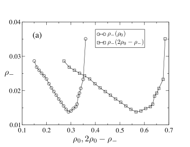
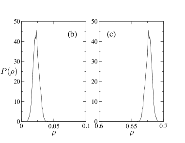
Figure 1: (a) Illustration of the operation of the intersection method described in the text for the determination of the coexistence diameter density. Data is shown for the state point $\eta_{s}^{r}=0.01$, $T=0.8(=0.764T_{c})$. Plotted are measured estimates of the average value $\rho_{-}$ of the low-density peak of $\hat{P}_{L}(\rho|\rho_{0})$, for a series of values of $\rho_{0}$. The same data is also shown plotted against $2\rho_{0}-\rho_{-}$. The value of $\rho_{0}$ at which the two data sets intersect [$\rho_{0}=0.351(3)$] serves as an estimate of the coexistence diameter density $\rho_{d}$. (b) and (c): The measured peaks of $\hat{P}_{L}(\rho)$ for $\rho_{0}=\rho_{d}$, whose individual integrated averages yield estimates of the coexistence densities.

Turning now to the matter of estimating critical parameters within the RGE, an accurate technique for achieving this has been described in detail in Ref. Ashton et al., 2010. The basic idea is to measure the “iso-$Q^{\star}$ curve” introduced in Ref. Liu et al., 2006, which is simply the locus of points in $\rho_{0}$–$T$ space for which the fourth-order cumulant ratio of $\hat{P}_{L}(\rho)$,

$$Q\equiv\frac{\langle(\rho-\rho_{0})^{2}\rangle^{2}}{\langle(\rho-\rho_{0})^{4}\rangle}\>,$$ (5)

matches the independently knownLiu et al. (2006) fixed-point value $Q^{\star}=0.711901$ appropriate to the Ising universality class and the RGE ensemble.

Now, it transpiresLiu et al. (2006); Ashton et al. (2010) that the iso-$Q^{\star}$ curve is essentially a parabola in $\rho_{0}$–$T$ space, the position of whose maximum represents a finite-size estimator of the critical-point density $\rho_{c}$ and temperature $T_{c}$. This maximum can be accurately located via a simple quadratic fit to measured points on the iso-$Q^{\star}$ curve. In practice we determine this curve as follows. A simulation is performed at some $\rho_{0}$ and $T$ to determine $\hat{P}(\rho)$. This distribution is then extrapolated in temperature via histogram reweightingFerrenberg and Swendsen (1989) to determine that temperature for which $Q=Q^{\star}$. The procedure is then repeated for a range of values of $\rho_{0}$ allowing us to trace out the whole iso-$Q^{\star}$ curve. An example of the resulting form of this curve is shown in Fig. 2. Note that, in general, for reasons of computational economy, the majority of the points that we determine on an iso-$Q^{\star}$ curve are for densities lower than the critical density, since the efficiency of the cluster algorithm is greater at lower overall volume fractions of particles.

Estimates of the critical parameters obtained from the iso-$Q^{\star}$ maxima for a range of system sizes can, in principle, be extrapolated to the thermodynamic limit using finite-size scaling relations derived in Ref. Ashton et al., 2010, which fully account for both field-mixing effects and corrections to scaling. Unfortunately, in the present work, the computational cost of simulating more than one system size was found to be prohibitive. However, the variations that we find in critical-point parameters as a function of $\eta_{s}^{r}$ dwarf those that one might expect on the basis of finite-size effects alone. Thus we are nevertheless able to report reliable trends from our measurements.

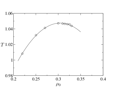
Figure 2: Estimates of points on the iso-$Q^{\star}$ curve for $\eta_{s}^{r}=0.01$, obtained for a system of size $L=10$, as described in the text. A parabolic fit to the data (solid line) identifies the coordinates of the maximum of the curve which serves as a finite-size estimate of the critical-point parameters.

III.3 Treatment of the small particles

As was argued in Sec. I, it is the relaxation of the large particles that constitutes the sampling bottleneck for highly size-asymmetrical mixtures. Local MC updates of small particles are computationally relatively unproblematic, irrespective of whether one performs particle displacements or insertions and deletions. Consequently, one has the choice of treating the small particles canonically so that their density is globally conserved, or grand canonically, in which case the density fluctuates under the control of a prescribed chemical potential. The choice one makes in this regard greatly affects the manner in which the bulk phase behavior is probed. Moreover it transpires that only the grand-canonical treatment of the small particles is compatible with our intersection method (Sec. III.2) for determining coexistence parameters.

To clarify these points, we show in Fig. 3 sketches of the isothermal bulk phase diagram of an exemplary size-asymmetrical binary mixture with large-particle density $\rho_{l}$, small-particle density $\rho_{s}$, and conjugate chemical potentials $\mu_{l}$ and $\mu_{s}$, respectively. Figure 3(ai) shows the phase behavior in the $\rho_{l}$–$\rho_{s}$ plane, while the corresponding phase diagram in the $\mu_{l}$–$\mu_{s}$ plane is shown in Fig. 3(aii). In constructing these sketches we have anticipated the behavior of the model of Sec. II, namely that the larger species has stronger attractive interactions and thus phase separates on its own [vertical axis of Fig. 3(ai)] at the chosen temperature, while the small-particle fluid (horizontal axis) does not. With interaction strengths chosen in this way, the larger particles will typically accumulate in the liquid phase, with its shorter interparticle distances, as shown by the representative tie lines in the density representation. Note that in chemical-potential space, coexistence occurs on a line of points, as shown in Fig. 3(aii).

Let us consider first the canonical scenario in which one traverses the coexistence region at constant bulk density of small particles, as expressed by the dashed trajectory included in Figs. 3(ai) and (aii). Clearly the tie lines in Fig. 3(ai) cross any line of constant $\rho_{s}$ moving from smaller values of $\rho_{l}/\rho_{s}$ at the gas end to larger ones for the coexisting liquid. Hence this path generates a sequence of pairs of coexistence states, one for each tie line crossed. The same trajectory in terms of the chemical potentials $\mu_{l}$–$\mu_{s}$ is shown in Fig. 3(aii). Here the path followed first meets the coexistence line, tracks along it it for some distance and then separates from it.

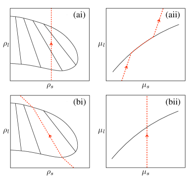
Figure 3: Isothermal cuts through the exemplary phase diagram of a binary fluid mixture described in the text. Liquid–vapor coexistence is represented in terms of (i) densities ($\rho_{l}$–$\rho_{s}$) and (ii) chemical potentials ($\mu_{l}$–$\mu_{s}$). In (a) the coexistence region is crossed along a path of constant $\rho_{s}$, whereas in (b) it is crossed along a path of constant $\mu_{s}$.

The alternative (grand-canonical) scenario, in which the small-particle density is permitted to fluctuate at constant chemical potential $\mu_{s}$, is illustrated in Figs. 3(bi) and (bii). Here, as $\mu_{l}$ is varied at constant $\mu_{s}$, the system crosses the coexistence line at a single point. In density space the corresponding trajectory thus follows a particular tie line though the coexistence region, as shown in Fig. 3(bi).

In seeking to apply the RGE ensemble to study a binary mixture, it is therefore imperative that one adopts a grand-canonical treatment of the small particles. Doing so ensures that only a single pair of coexistence states is encountered inside the bulk coexistence region, i.e., that one tracks a tie line of the bulk phase diagram. This is a prerequisite for the correct operation of our intersection method, which is designed to determine first the diameter density for a single pair of coexistence states as a prelude to determining the coexistence densities of the large particles themselves. We further note that a grand-canonical treatment of the small particles corresponds more closely to common experimental arrangements where one typically measures properties of the mixture with respect to variations of a reservoir volume fraction of small particles.

IV Results

Equipped with the methods described above, we can set about the task of determining the coexistence properties of the large particles in the presence of a sea of small ones. To this end we apply the GCA–RGE method to study liquid–vapor phase coexistence in a $q=0.1$ LJ mixture (see Sec. II). In addition to the cluster updates which swap whole groups of particles (including both large and small species) between boxes, small particles are sampled across both boxes using a standard local grand-canonical algorithm at constant chemical potential (see Sec. III.3). As discussed above, we choose $\mu_{s}$ to yield (for each temperature of interest) a prescribed volume fraction $\eta^{r}_{s}$ of small particles in the reservoir. This requires prior knowledge of the reservoir equation of state $\eta_{s}^{r}(\mu_{s},T)$, which we obtained via explicit simulation of the pure fluid of small particles. Note that the computational cost of obtaining $\eta_{s}^{r}(\mu_{s},T)$ is low, particularly if one employs histogram extrapolationFerrenberg and Swendsen (1989) to scan a region of $\mu$ and $T$ surrounding each simulation state point.

The GCA–RGE simulations are performed using two cubic periodic simulation boxes of linear size $L=10$. We consider seven values of the reservoir volume fraction of the small particles, $\eta^{r}_{s}=0.005$, $0.01$, $0.015$, $0.02$, $0.03$, $0.04$, and $0.05$. In the limit of low densities of large particles, these values of $\eta^{r}_{s}$ correspond to average numbers of small particles in the range $10^{4}$–$10^{5}$. The computational expenditure incurred in simulating such great numbers of small particles places an upper bound on the value of $\eta_{s}^{r}$ for which it is feasible to perform a full determination of the coexistence binodal. Further difficulties arise from the fact that the typical cluster size at coexistence was found to grow steadily as we increased $\eta_{s}^{r}$. This is demonstrated in Fig. 4 which plots the distribution of the fraction of large particles in the cluster for $\eta_{s}^{r}=0.01,0.03$ and $0.05$ measured at the respective critical point parameters. These distributions are bimodal, with some fairly small clusters comprising just a few particles, and many clusters that comprise the vast proportion of large particles. Updating such clusters results in only relatively minor alterations to a configuration and consequently, we are able to determine the coexistence binodal only for $\eta_{s}^{r}\leq 3\%$, whereas for $\eta_{s}^{r}=0.04$ and $0.05$ we restrict ourselves to determining critical-point parameters. It should be stressed however, that the cluster sizes observed in the present study may not provide a general guide to the maximum $\eta_{s}^{r}$ at which the GCA-RGE scheme will operate. This is because, as we shall show, our choice of interspecies interactions engenders a large depression in $T_{c}$ with increasing $\eta_{s}^{r}$ which in turn promotes the formation of large clusters due to the temperature dependence of the GCA bond-formation probability Eq. (2). However, other choices of interactions can be expected to lead to a different temperature dependence of the critical point parameters, hence allowing larger values of $\eta_{s}^{r}$ to be attained.

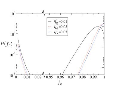
Figure 4: Distribution of the fraction of large particles in the cluster, $f_{c}$, at criticality for the values of $\eta_{s}^{r}$ shown in the legend.

The critical-point parameters are determined, for each $\eta_{s}^{r}$ studied, from measurements of the iso-$Q^{\star}$ curve. For $\eta_{s}^{r}\leq 3\%$, the intersection method described in Sec. III.2 is deployed to determine the large-particle coexistence densities in the subcritical regime. Figure 5 presents our results for the $\rho$–$T$ binodal. The principal feature is – as previously mentioned – a strong depression of the binodal to lower temperatures and lower densities as $\eta_{s}^{r}$ is increased. The scale of the associated shifts in the critical parameters is made apparent in Fig. 6, which plots our estimates of the critical temperature and density as a function of $\eta_{s}^{r}$. One sees that as the reservoir volume fraction of small particles is increased in the range $0$ – $0.05$, the critical temperature decreases by approximately $50\%$, while the critical density drops by some $30\%$. The error bars shown on the estimates of the critical parameters derive from a bootstrap analysis of the various quadratic fits that are consistent with the uncertainties in the locus of each iso-$Q^{\star}$ curve (Fig. 7).

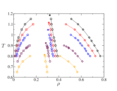
Figure 5: Phase diagrams showing the liquid (diamonds) and gas (squares) coexistence densities of large particles for $q=0.1$. Data are shown for reservoir volume fractions (top to bottom) $\eta_{s}^{r}=0$, $0.005$, $0.01$, $0.02$, and $0.03$. Also shown in each case is the coexistence diameter (circles) and critical point (asterisks).

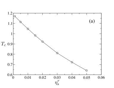
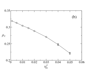
Figure 6: (a) Critical temperature and (b) critical density versus $\eta_{s}^{r}$ as determined from the iso-$Q^{\star}$ curves. Error bars derive from a bootstrap analysis with 100 resamples.

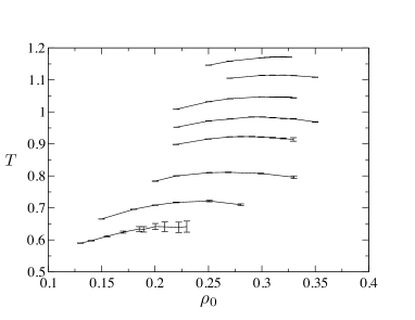
Figure 7: The measured iso-$Q^{\star}$ curves for (top to bottom) $\eta^{r}_{s}=0$, $0.005$, $0.01$, $0.015$, $0.02$, $0.03$, $0.04$, and $0.05$. Also shown are the estimated error bars from which we calculated the overall uncertainty in critical parameters via a bootstrap analysis.

To demonstrate the correctness of our method, we compare the binodal for $\eta_{s}^{r}=0.01$ with that obtained using a quite different approach, recently proposed by two of usAshton and Wilding (2010). This is a fully grand-canonical MC scheme in which large particles are gradually transferred to and from the system by means of staged insertions and deletions. To negate ensemble differences that occur when comparing results in finite-size systems, we transform the grand-canonical distribution of the large-particle density, $P(\rho)$, to the RGE using the exact transformation $\hat{P}(\rho)=P(\rho)P(2\rho_{0}-\rho)$Liu et al. (2006); Ashton et al. (2010). We then proceed to locate coexistence as if the data had been generated in the RGE by treating $\rho_{0}$ as a parameter of the transformation. The resulting coexistence densities are compared with those obtained via the GCA–RGE simulations in Fig. 8. The agreement is good, particularly at low temperature. The deviations near criticality arise from the difference in the system size used in each case ($L=7.5\sigma_{ll}$ for the grand-canonical system and $L=10\sigma_{ll}$ for the RGE system), and thus reflect that the correlation length exceeds the system size in the grand-canonical simulation.

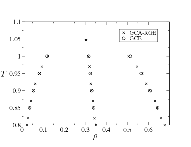
Figure 8: Comparison for $\eta_{r}^{s}=0.01$ of the binodal obtained using the GCA–RGE technique (crosses) and the grand-canonical approach (circles) described in Ref. Ashton and Wilding, 2010. Statistical uncertainties are comparable to the symbol sizes. Differences in the results near criticality arise from the different system sizes used in the two cases.

It is instructive to attempt to relate the shift in the binodal occurring with increasing small-particle density to alterations in the underlying local fluid structure. An indication as to the factors at work here follows from a study of the effect of small particles on the effective potential between a pair of large particles,

$$\beta W(r)\equiv\lim_{\rho\to 0}-\ln[g_{ll}(r)]\;.$$ (6)

An example is shown in Fig. 9(a) which compares $\beta W(r)$ for the cases $\eta_{s}^{r}=0$ (which simply corresponds to the bare Lennard-Jones potential) with that for $\eta_{s}^{r}=0.05$, at $T=1.3$. One sees that for typical separations of large particles, the effective potential is less attractive than the bare interaction. Thus the net effect of the small particles is repulsive as shown by the difference plot in fig. 9(a), a feature that accords with the reduction in the critical temperature. A likely reason for this is to be found in the associated form of $g_{ls}(r)$ describing the correlations between a large particle and a small particle, as shown in Fig. 9(b) at $\eta_{s}^{r}=0.05$. This shows that small particles form a diffuse, non absorbing cloud around each large particle because of their weak mutual attraction. Presumably, however, the free-energy cost arising when the clouds associated with two or more large particles overlap acts to reduce the intrinsic attractions between large particles. Interestingly, the difference plot of Fig. 9(a) shows that at very small separations of large particles (corresponding to high overlap energy) the effect of the small particles changes from being repulsive to being attractive.

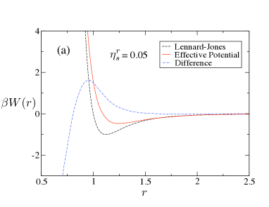
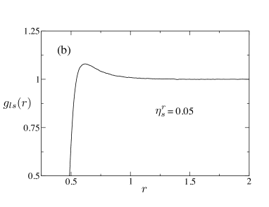
Figure 9: (a) The measured form of the effective potential $\beta W(r)$ defined in the text, at temperature $T=1.3$. Data are shown for the bare LJ potential ($\eta_{s}^{r}=0$, dashed line) and $\eta_{s}^{r}=0.05$ (solid line) and their difference (dashed-dotted line). (b) Form of $g_{ls}(r)$ for $\rho_{ll}\to 0$ at $\eta_{s}^{r}=0.05,T=1.3$.

Finally, we show in Fig. 10 a configurational snapshot of our simulation boxes at coexistence (i.e., $\rho_{0}=\rho_{d}$) for the case $\eta^{r}_{s}=3\%$, $T=0.88T_{c}$. This provides a visual impression of the character of the coexisting phases and the extent to which the large particles are severely “jammed” by the small ones.

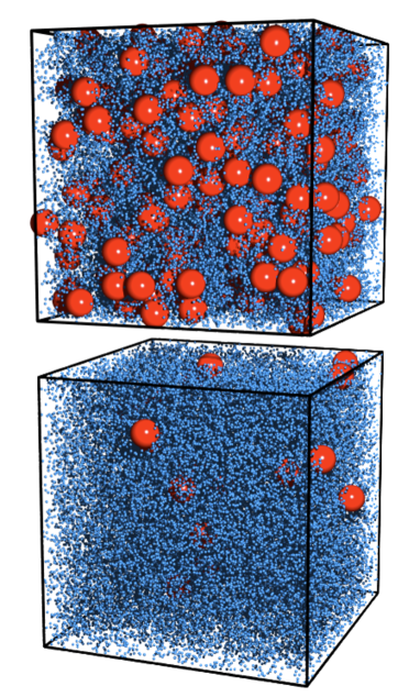
Figure 10: Configurational snapshot of the two boxes in the restricted Gibbs ensemble at coexistence for $\eta^{r}_{s}=3\%$, $T=0.88T_{c}$.

V Discussion and conclusions

In summary, we have described a variant of the Geometric Cluster AlgorithmLiu and Luijten (2004) for the accurate determination of phase behavior in highly size-asymmetrical fluid mixtures. The method (an early version of which was previously described in Ref. Liu et al., 2006) operates by swapping clusters containing large and small particles between two boxes of equal volume, the global density of large particles being fixed. The resulting spectrum of single-box fluctuations of the large particles can be analyzed with respect to changes in their global density using the intersection method of Ashton et al.Ashton et al. (2010) to yield accurate estimates of coexistence densities. Critical points can similarly be located to high precision by using an appropriate finite-size estimator for criticality, namely the maximum of the iso-$Q^{\star}$ curve.

We have applied the method to a LJ mixture with size ratio $10$:$1$ to determine the coexistence properties of large particles for small-particle reservoir volume fractions in the range $0\leq\eta_{s}^{r}\leq 3\%$. Additionally, critical-point parameters were determined for $\eta_{s}^{r}=0.04$ and $0.05$. Our results show that when the small particles are weakly attracted to the large ones, their net effect is to lower the degree of attraction between large particles. As a consequence, the coexistence binodal shifts to lower temperatures, confirming the preliminary findings of Ref. Liu et al., 2006. Such a situation contrasts markedly with the depletion effect applicable to small particles that interact with the large ones like hard spheresAsakura and Oosawa (1954), for which there is a net increase in the degree of attraction between large particles. Our measurements of local structure suggest that in the case we have considered, the small particles form a diffuse (nonadsorbing) cloud surrounding each large particle. The overlap of clouds necessary for two large particles to approach one another appears unfavorable in free-energy terms, leading to a net decrease in the degree of attraction between large particles. This is reminiscent of the “nanoparticle haloing” effectTohver et al. (2001); Liu and Luijten (2004).

It is gratifying to note that the GCA–RGE method permits the study of phase behavior in regimes that are inaccessible to traditional simulation approaches. Specifically, the phase diagrams we have presented could not have been obtained using even the most efficient traditional approach to fluid phase equilibria, namely standard grand-canonical simulationWilding (1995). For instance, for $\eta_{s}^{r}>0.005$ our tests show that the grand-canonical relaxation time is too large to be reliably estimated. Nevertheless, a lower bound on the grand-canonical relaxation time, relative to that of the pure LJ fluid, can be estimated via a comparison of the large-particle transfer (insertion/deletion) acceptance probability $p_{\rm acc}$. For liquid-like densities of the large particles ($\rho\approx 0.6$), $p_{\rm acc}$ is of the order of $10^{-4}$ at $\eta_{s}^{r}=0.005$Liu et al. (2006). Upon increasing $\eta_{s}^{r}$ to a volume fraction of merely 1%, this probability falls to $p_{\rm acc}\sim 10^{-6}$. These values are to be compared with $p_{\rm acc}\sim 10^{-1}$ for the pure LJ fluid. One can therefore expect the grand-canonical relaxation time of the mixtures studied here to be several orders of magnitude greater than for the pure LJ fluid.

Notwithstanding the efficiency gains provided by the GCA-RGE approach, it should be stressed that the results we have reported nevertheless entailed a significant computational outlay. Specifically, runs to determine each coexistence point typically varied in length between 100 and 3,000 hours of CPU time on a 3 GHz processor. The upper value in this range was that required at the highest volume fraction of small particles studied (for which there are very many small particles) and the lowest temperature (where most of the large particles are involved in each cluster update). Thus whilst studies of phase behaviour in highly asymmetrical mixtures cannot yet be regarded as routine, they are now at least feasible.

With regard to future studies of highly asymmetrical mixtures, one barrier to attaining higher values of $\eta_{s}^{r}$ and smaller values of $q$ is simply the computational overhead associated with large numbers of small particles, although we note that the GCA has been successfully applied to systems with millions of nanoparticlesLiu and Luijten (2004). Additionally, in the present model, the suppression of the critical temperature with increasing $\eta_{s}^{r}$ leads to a rapid growth in the cluster size which renders the GCA–RGE approach increasingly less efficient. More generally, however, in situations where the small particles induce an effective (depletion) attraction between the large ones, we expect that the cluster size will remain manageable to rather larger $\eta_{s}^{r}$ than studied here.

Finally, we mention an alternative approach, proposed by two of us, for determining coexistence properties in highly size-asymmetrical mixturesAshton and Wilding (2010). This method utilizes an expanded grand-canonical ensemble in which the insertion and deletion of large particles is accomplished gradually by traversing a series of states in which a large particle interacts only partially with the environment of small particles. Implementing this approach requires prior determination of a multicanonical weight function to bias insertions of the particles, and thus renders it less straightforward to use than the GCA–RGE. However, being fully grand canonical does have the advantage of providing information on the chemical potentials of large particles, thereby permitting histogram reweighting in terms of density as well as temperature. In future work we hope to provide a systematic comparison of the relative computational cost of both approaches in various parameter regimes.