Finite temperature damping of collective modes of a BCS-BEC crossover superfluid

Abstract

A new mechanism is proposed to explain the puzzling damping of collective excitations, which was recently observed in the experiments of strongly interacting Fermi gases below the superfluid critical temperature on the fermionic (BCS) side of Feshbach resonance. Sound velocity, superfluid density and damping rate are calculated with effective field theory. We find that a dominant damping process is due to the interaction between superfluid phonons and thermally excited fermionic quasi-particles, in contrast to the previously proposed pair-breaking mechanism. Results from our effective model are compared quantitatively with recent experimental findings, showing a good agreement.

I Introduction

In recent years, experimental studies on ultracold Fermi gases in Bose-Einstein condensation (BEC) to Bardeen-Cooper-Schrieffer (BCS) crossover Nozières and Schmitt-Rink (1985); Sá de Melo et al. (1993); Giorgini et al. (2008) have shown many interesting results O’Hara et al. (2002); Regal et al. (2004); Zwierlein et al. (2004); Nascimbène et al. (2009). By varying external magnetic field to effectively tune the scattering length through Feshbach Resonance, or changing the temperature, collective behaviors, such as oscillation frequency, sound velocity and damping rate, have been extensively investigated Bartenstein et al. (2004); Kinast et al. (2005); Joseph et al. (2007); Wright et al. (2007); Altmeyer et al. (2007). Recently, several experiments show a puzzling damping of collective excitations occurs in superfluid regime where the system is at a finite temperature and on the (fermion) BCS side of the crossover Bartenstein et al. (2004); Wright et al. (2007); Altmeyer et al. (2007).

In the theoretical front, the properties of collective excitations in the crossover have been investigated by a variety of established methods Giorgini et al. (2008), including work that used the hydrodynamic theory Stringari (2004); Heiselberg (2004); Hu et al. (2004), the Gaussian fluctuation approximation from a microscopic Lagrangian Engelbrecht et al. (1997); Taylor et al. (2006); Fukushima et al. (2007); Diener et al. (2008), and fermion-boson coupled model Holland et al. (2001); Ohashi and Griffin (2002, 2003). The Boltzmann equation Vichi (2000); Massignan et al. (2005); Bruun and Smith (2007); Riedl et al. (2008) and semiclassical dynamics Urban and Schuck (2006); Urban (2008) were also used to explain the frequency and damping rate of oscillation modes.

Effective field theory has also been used in some previous work to study ultracold systems at zero temperature, including expanding the goldstone fields to higher orders, or low energy expansion Liu (2006); Mañes and Valle (2009); Schakel (2011). In this paper, we use effective field theory to study the collective modes of the superfluid state of an unpolarized strongly interacting cold Fermi gas at finite temperatures near the Feshbach resonance regime. Our effective theory is constructed based on a single-channel resonance model, which is known to be adequate for a broad Feshbach resonance. Furthermore, we focus on the BCS side of the crossover, where puzzling damping phenomena have been observed and received much attention Bartenstein et al. (2004); Wright et al. (2007); Altmeyer et al. (2007). In this regime, the BEC molecular effect is negligible, and hence the single-channel calculation which we adopt is simple and valid. Our main results are as follows. First, our theory shows that a dominant damping process is due to interaction between superfluid phonons and thermally excited fermionic quasi-particles at finite temperatures, in contrast to the previously proposed pair-breaking mechanism. Such a process is related to the well-known Landau damping, which was previously discussed in a semiclassical approach by taking the $\hbar\rightarrow 0$ limit of the time-dependent Hartree-Fock-Bogoliubov equations Urban and Schuck (2006); Urban (2008). Second, we calculate the damping rate of collective excitations for the physical systems and find a good comparison with the recent experimental findings. Throughout the paper, the Planck constant $\hbar$ and Boltzmann constant $k_{B}$ are set unity ($\hbar\equiv k_{B}\equiv 1$ in units).

II MEAN FIELD THEORY

We consider an unpolarized ultracold fermionic system with two spin species (spin $\uparrow$ and $\downarrow$) of equal mass. The partition function of the system in the grand canonical ensemble can be described in the path integral formalism

$$Z=\int D(\psi_{\sigma}^{*},\psi_{\sigma})\exp(-S_{\psi})$$ (1)

where $S_{\psi}=\int dx\mathcal{L}_{\psi}(x)$ is the action. $\psi_{\sigma}$ is the fermionic field for spin $\sigma=\uparrow,\downarrow$. $x$ is a four vector $x=(\mathbf{x},\tau)$, in which $\mathbf{x}$ is the spatial coordinate and $\tau$ is imaginary time in the range $0<\tau<\beta$, $\beta=1/T$ and $T$ is the temperature of the system. The following Lagrangian is used to describe the system:

$$\mathcal{L}_{\psi}={\psi^{*}_{\sigma}\left(\partial_{\tau}-\frac{\nabla^{2}}{2m_{a}}-\mu\right)\psi_{\sigma}}+g\psi^{*}_{\uparrow}\psi^{*}_{\downarrow}\psi_{\downarrow}\psi_{\uparrow},$$ (2)

where $m_{a}$ is the mass of the fermion, $g$ is the interaction (negative on the BCS side), and $\mu$ is the chemical potential. The summation over $\sigma$ is implicit.

As usual, we use a Hubbard-Stratonovich transformation by introducing an auxiliary complex bosonic field $\Delta(x)$ to eliminate the quartic term in Eq. (2) and get

$$Z=\int D(\psi_{\sigma}^{*},\psi_{\sigma})D(\Delta^{*},\Delta)\exp(-S_{\psi,\Delta}),$$ (3)

where the lagrangian is now

$$\mathcal{L}_{\psi,\Delta}=\psi^{*}_{\sigma}\left(\partial_{\tau}-\frac{\nabla^{2}}{2m_{a}}-\mu\right)\psi_{\sigma}+(\psi^{*}_{\uparrow}\psi^{*}_{\downarrow}\Delta+c.c)-\frac{|\Delta|^{2}}{g}.$$ (4)

In this transformation, the (auxiliary) field $\Delta(x)$ acquires exactly the same expectation value as the pair field at the saddle point:

$$\langle\Delta\rangle=\langle\psi_{\downarrow}\psi_{\uparrow}\rangle\,.$$

The fermionic field is now in quadratic form and can be integrated out to get an effective action for the field $\Delta$

$$Z=\int D(\Delta^{*},\Delta)\exp(-S_{\Delta}),$$ (5)

where

$$S_{\Delta}=-\int d^{4}x\left(\frac{|\Delta|^{2}}{g}+\textrm{tr}\ln G^{-1}\right)$$ (6)

and

$$G^{-1} = \left(\begin{array}[]{cc}\partial_{\tau}-\frac{\nabla^{2}}{2m_{a}}-\mu&\Delta\\ \Delta^{*}&\partial_{\tau}+\frac{\nabla^{2}}{2m_{a}}+\mu\end{array}\right).$$ (9)

In the mean field approximation, we seek for a spatially uniform saddle point solution $\Delta_{0}$ of $S_{\Delta}$, together with the requirement of fixing the number density $n$. These two conditions determine the mean field equations in the crossover

$$\frac{\delta S_{\Delta}}{\delta\Delta_{0}}=0,$$

$$\frac{\partial\ln Z}{\partial\mu}=n.$$ (10)

In momentum space we get

$$\frac{1}{g}+\sum_{\mathbf{k}}\frac{1}{2E_{k}}\tanh\left(\frac{\beta E_{k}}{2}\right) = 0,$$

$$\sum_{\mathbf{k}}\left[1-\frac{\xi_{k}}{E_{k}}\tanh\left(\frac{\beta E_{k}}{2}\right)\right] = n,$$ (11)

where $E_{k}=\sqrt{\xi_{k}^{2}+\Delta^{2}}$ and $\xi_{k}=\frac{k^{2}}{2m_{a}}-\mu$.

We use the usual regularization procedure,

$$\frac{m_{a}}{4\pi a}=\frac{1}{g(\Lambda)}+\sum_{|\mathbf{k}|<\Lambda}\frac{1}{2\epsilon_{k}}\,,$$ (12)

where $\epsilon_{k}=|\mathbf{k}|^{2}/2m_{a}$ and $a$ is the effective scattering length. Taking $\Lambda\rightarrow\infty$, Eq. (11) can be expressed in terms of $a$ as

$$\frac{m_{a}}{4\pi a} = \sum_{\mathbf{k}}\left[\frac{1}{2\epsilon_{k}}-\frac{1}{2E_{k}}\tanh\left(\frac{\beta E_{k}}{2}\right)\right],$$

$$n = \sum_{\mathbf{k}}\left[1-\frac{\xi_{k}}{E_{k}}\tanh\left(\frac{\beta E_{k}}{2}\right)\right].$$ (13)

By self consistently solving Eq. (13), we can get $\Delta_{0}$ and $\mu$ as function of $1/k_{F}a$ and $T/T_{F}$ in mean field level, where $k_{F}$ and $T_{F}$ are the Fermi momentum and temperature of the non-interacting Fermi gas in free space with the same number density $n$. In the following sections, we will assume the state of the system is already superfluid and will use the mean field results, such as the gap parameter, as input to calculate the physical quantities of excitations.

III Quantum Fluctuations

To consider the quantum fluctuations, we no longer treat the order parameter $\Delta$ as a homogeneous constant in Eq. (4), but write it as

$$\Delta(x)=\Delta_{0}\left(1+\lambda(x)\right)e^{i2\varphi(x)}.$$ (14)

$\lambda$ is the amplitude fluctuation and $\varphi$ is the phase fluctuation around the saddle point solution $\Delta_{0}$, and both of them are real. Then one can apply a local U(1) gauge transformation to a new gauge where the order parameter is real everywhere in space

$$\Delta=\tilde{\Delta}e^{i2\varphi(x)},\psi_{\sigma}(x)=\tilde{\psi}_{\sigma}(x)e^{i\varphi(x)},$$ (15)

and $\tilde{\Delta}=\Delta_{0}(1+\lambda)$ is real now . In the new gauge, the Lagrangrian density Eq. (4) becomes

$$\mathcal{L}_{\tilde{\psi},\varphi,\lambda} = \tilde{\psi}^{*}_{\sigma}(\partial_{\tau}-\frac{\nabla^{2}}{2m_{a}}-\mu)\tilde{\psi}_{\sigma}+(\Delta_{0}\tilde{\psi}^{*}_{\uparrow}\tilde{\psi}_{\downarrow}^{*}+c.c.)$$ (16)

$$+\tilde{\psi}^{*}_{\sigma}\tilde{\psi}_{\sigma}[i\partial_{\tau}\varphi+\frac{(\nabla\varphi)^{2}}{2m_{a}}]+\nabla\varphi\cdot\hat{\mathbf{J}}_{\sigma}$$

$$+(\Delta_{0}\lambda\tilde{\psi}^{*}_{\uparrow}\tilde{\psi}_{\downarrow}^{*}+c.c.)-\frac{\Delta_{0}^{2}\lambda^{2}}{g}$$

where $\hat{\mathbf{J}}_{\sigma}=\hat{\mathbf{J}}_{\sigma}(x)=-\frac{i}{2m_{a}}[\tilde{\psi}^{*}_{\sigma}(\nabla\tilde{\psi}_{\sigma})-(\nabla\tilde{\psi}^{*}_{\sigma})\tilde{\psi}_{\sigma}]$ is the fermion current field.

We now integrate out the fermionic field which is gapped. In momentum space, for the fermionic field $\tilde{\psi}$, we use $k=(\mathbf{k},i\omega_{m})$, where $\omega_{m}=(2m+1)\pi/\beta$ is the fermionic Matubara frequecy and $m$ is integer. For the bosonic field $\lambda$ and $\varphi$, we use $q=(\mathbf{q},i\omega_{n})$, and $\omega_{n}=2n\pi/\beta$, where $n$ is integer.

Introducing two component spinor in momentum space $\Psi_{k}^{*}=(\tilde{\psi}_{k\uparrow}^{*},\tilde{\psi}_{-k\downarrow})$, we can rewrite the action in momentum space as $S=\sum_{k_{1},k_{2}}\Psi_{k_{1}}^{*}G^{-1}(k_{1},k_{2})\Psi_{k_{2}}$, where $G^{-1}=G_{0}^{-1}+\chi_{1}+\chi_{2}$ is $2\times 2$ matrix. $G_{0}$, $\chi_{1}$, and $\chi_{2}$ are given by

$$G_{0}(k_{1},k_{2}) = \frac{\delta_{k_{1},k_{2}}}{\omega_{m_{1}}^{2}+E_{k_{1}}^{2}}\left(\begin{array}[]{cc}i\omega_{m_{1}}+\xi_{k_{1}}&\Delta_{0}\\ \Delta_{0}&i\omega_{m_{1}}-\xi_{k_{1}}\end{array}\right)$$ (19)

$$\chi_{2}(k_{1},k_{2}) = -\sum_{q}\frac{\mathbf{q}\cdot(\mathbf{k_{1}-k_{2}-q})}{2m_{a}\beta V}\varphi_{q}\varphi_{k_{1}-k_{2}-q}\left(\begin{array}[]{cc}1&0\\ 0&-1\end{array}\right)$$ (22)

$$\chi_{1}(k_{1},k_{2}) = \left(\begin{array}[]{cc}\chi_{1}^{11}(k_{1},k_{2})&\chi_{1}^{12}(k_{1},k_{2})\\ \chi_{1}^{21}(k_{1},k_{2})&\chi_{1}^{22}(k_{1},k_{2})\end{array}\right)$$ (25)

with

$$\chi_{1}^{11}(k_{1},k_{2}) = \left[\frac{\omega_{m_{1}}-\omega_{m_{2}}}{\sqrt{\beta V}}+\frac{i(\mathbf{k_{1}^{2}-k_{2}^{2}})}{2m\sqrt{\beta V}}\right]\varphi_{k_{1}-k_{2}}$$

$$\chi_{1}^{22}(k_{1},k_{2}) = \left[-\frac{\omega_{m_{1}}-\omega_{m_{2}}}{\sqrt{\beta V}}+\frac{i(\mathbf{k_{1}^{2}-k_{2}^{2}})}{2m\sqrt{\beta V}}\right]\varphi_{k_{1}-k_{2}}$$

$$\chi_{1}^{12}(k_{1},k_{2}) = \chi_{1}^{21}(k_{1},k_{2})=\frac{\Delta_{0}}{\sqrt{\beta V}}\lambda_{k_{1}-k_{2}}.$$ (26)

Keeping the $\lambda$ and $\varphi$ field to quadratic order 

$$\int D(\Psi^{*},\Psi)e^{-S_{\Psi,\lambda,\varphi}}\approx e^{\textrm{tr}[G_{0}\chi_{2}-\frac{1}{2}G_{0}\chi_{1}G_{0}\chi_{1}]}=e^{-S^{\prime}},$$ (27)

we get the effective action

$$S^{\prime}=S_{\varphi}+S_{\lambda}+S_{\varphi,\lambda},$$ (28)

where

$$S_{\varphi} = \sum_{q}\varphi_{q}\varphi_{-q}[f_{1}(q)\omega_{n}^{2}+[f_{4}(q)+\frac{n}{2m_{a}}]\mathbf{q}^{2}],$$

$$S_{\lambda} = \sum_{q}\lambda_{q}\lambda_{-q}f_{3}(q),$$

$$S_{\varphi,\lambda} = \sum_{q}[f_{2}(q)\lambda_{q}\varphi_{-q}(-\omega_{n}-\frac{i}{m_{a}}\mathbf{q\cdot k})$$ (29)

$$-f_{2}(q)\lambda_{-q}\varphi_{q}(-\omega_{n}+\frac{i}{m_{a}}\mathbf{q\cdot k})],$$

and 

$$f_{1} = \frac{1}{\beta V}\sum_{k}\frac{\omega_{m}\omega_{m+n}-\xi_{k}\xi_{k+q}+\Delta_{0}^{2}}{(\omega_{m}^{2}+E_{k}^{2})(\omega_{m+n}^{2}+E_{k+q}^{2})},$$

$$f_{2} = \frac{\Delta_{0}^{2}}{\beta V}\sum_{k}\frac{i\omega_{m}+i\omega_{m+n}+\xi_{k}+\xi_{k+q}}{(\omega_{m}^{2}+E_{k}^{2})(\omega_{m+n}^{2}+E_{k+q}^{2})},$$

$$f_{3} = -\frac{\Delta_{0}^{2}}{g}-\frac{\Delta_{0}^{2}}{\beta V}\sum_{k}\frac{\omega_{m}\omega_{m+n}+\xi_{k}\xi_{k+q}-\Delta_{0}^{2}}{(\omega_{m}^{2}+E_{k}^{2})(\omega_{m+n}^{2}+E_{k+q}^{2})},$$

$$f_{4} = \frac{1}{\beta V}\sum_{k}\frac{k^{2}\cos^{2}\theta}{m_{a}^{2}}\frac{-\omega_{m}\omega_{m+n}+\xi_{k}\xi_{k+q}+\Delta_{0}^{2}}{(\omega_{m}^{2}+E_{k}^{2})(\omega_{m+n}^{2}+E_{k+q}^{2})}.$$

The next step is to integrate out the amplitude fluctuation field $\lambda$ and keep only the phase field. Define

$$C_{1}(q) = f_{1}+f_{2}^{2}/f_{3},$$

$$C_{2}(q) = f_{4}+\frac{n}{2m_{a}},$$ (31)

and the effective action of phase field $\varphi$ is obtained as

$$S_{\varphi}=\sum_{q}\varphi_{q}\varphi_{-q}[C_{1}(q)\omega_{n}^{2}+C_{2}(q)\mathbf{q}^{2}].$$ (32)

IV Superfluid density and sound velocity

Some physical quantities such as superfluid density and sound velocity can be evaluated by our theory. To get a full expression for the superfluid density, one can apply a Galilean boost on the order parameter in Eq. (15), and get the superfluid density by the shift of free energy in the superfluid hydrodynamic model with normal and superfluid components Taylor et al. (2006); Fukushima et al. (2007); Taylor (2007). The total normal density includes bosonic fluctuation part and non-condensed fermionic Bogoliubov quasi-particle part. From the calculations of Ref. Taylor et al. (2006); Fukushima et al. (2007); Taylor (2007), the main contribution to the normal density on the BEC side is the bosonic fluctuation part, while on the BCS side, the main contribution is from the non-condensed fermionic quasi-particle part. Since our main focus is the damping on the BCS side, we will neglect the part of bosonic fluctuations in the normal density in the following calculation.

To the zeroth order of $q$, or in the long wave length limit $q\rightarrow 0$, all coefficients $f_{1},f_{2},f_{3}$, and $f_{4}$ are real, in terms of which superfluid density and sound velocity can be expressed. Since the imaginary part is zero, there is no damping for the collective modes, to the lowest order. $C_{1}^{\prime}\equiv\lim_{q\rightarrow 0}C_{1}$ is related to the density of states, and $C_{2}^{\prime}\equiv\lim_{q\rightarrow 0}C_{2}=n_{s}/2m_{a}$ is related to superfluid density $n_{s}$ Altland and Simons (2006) .

Take the limit of $q\rightarrow 0$ in the coefficients Eq. (LABEL:eq:f1tof5), and define $f_{1}^{\prime}\equiv\lim_{q\rightarrow 0}f_{1}$ and so on. After carrying out the Matsubara summation for $i\omega_{m}$, we get 

$$f_{1}^{\prime} = \frac{1}{V}\sum_{\mathbf{k}}[\beta n_{k}(1-n_{k})\frac{\xi_{k}^{2}}{E_{k}^{2}}+\frac{\Delta_{0}^{2}}{2E_{k}^{3}}(1-2n_{k})]\,,$$

$$f_{2}^{\prime} = \frac{\Delta^{2}_{0}}{V}\sum_{\mathbf{k}}[\beta n_{k}(n_{k}-1)\frac{\xi_{k}}{E_{k}^{2}}+(1-2n_{k})\frac{\xi_{k}}{2E_{k}^{3}}]\,,$$

$$f_{3}^{\prime} = \frac{\Delta_{0}^{4}}{V}\sum_{\mathbf{k}}[\beta n_{k}(n_{k}-1)\frac{1}{E_{k}^{2}}+\frac{1}{2E_{K}^{3}}\tan\frac{\beta E_{k}}{2}]\,,$$

$$f_{4}^{\prime} = \sum_{\mathbf{k}}\frac{\beta}{V}\frac{k^{2}\cos^{2}\theta}{m_{a}^{2}}n_{k}(n_{k}-1)\,,$$

where

$$n_{k}={1\over e^{\beta E_{k}}+1}$$

is the quasi-particle Fermi-Dirac distribution. Eq. (32) becomes

$$S=\sum_{q}\varphi_{q}\varphi_{-q}[C_{1}^{\prime}\omega_{n}^{2}+C_{2}^{\prime}\mathbf{q}^{2}]$$ (34)

with

$$C_{1}^{\prime} = f_{1}^{\prime}+f_{2}^{\prime 2}/f_{3}^{\prime}\,,$$

$$C_{2}^{\prime} = f_{4}^{\prime}+\frac{n}{2m_{a}}\,.$$ (35)

After applying a Wick rotation $i\omega_{n}=\omega_{q}+i0^{+}$, the zero of the action, Eq. (34), gives the spectrum $\omega_{q}=v_{s}|\mathbf{q}|$, where $v_{s}$ is the sound velocity. Thus, we get the following physical quantities,

$$\frac{n_{s}}{2m_{a}} = f_{4}^{\prime}+\frac{n}{2m_{a}}\,,$$

$$v_{s}^{2} = \frac{f_{4}^{\prime}+n/2m_{a}}{f_{1}^{\prime}+f_{2}^{\prime 2}/f_{3}^{\prime}}\,.$$ (36)

At zero temperature, Eq. (LABEL:eq:coeffreal) reduces to

$$f_{1,T=0}^{\prime} = \frac{\Delta_{0}^{2}}{V}\sum_{\mathbf{k}}\frac{1}{2E_{k}^{3}},$$

$$f_{2,T=0}^{\prime} = \frac{\Delta^{2}_{0}}{V}\sum_{\mathbf{k}}\frac{\xi_{k}}{2E_{k}^{3}},$$

$$f_{3,T=0}^{\prime} = \frac{\Delta_{0}^{4}}{V}\sum_{\mathbf{k}}\frac{1}{2E_{k}^{3}},$$

$$f_{4,T=0}^{\prime} = 0.$$

Perform the summation for $f^{\prime}$’s over $\mathbf{k}$ as integration in the thermodynamic limit, and define the following integral quantities

$$J_{2} = \int_{0}^{\infty}dk\frac{k^{2}}{E_{k}^{3}},$$

$$J_{4} = \int_{0}^{\infty}dk\frac{k^{4}}{E_{k}^{3}},$$

$$J_{\xi} = \int_{0}^{\infty}dk\frac{k^{2}\xi_{k}}{E_{k}^{3}}.$$ (38)

After some calculations, the sound velocity at $T=0$ is

$$v_{s,T=0}^{2}=\frac{1}{3m_{a}^{2}}\frac{J_{2}J_{4}\Delta_{0}^{2}}{J_{2}^{2}\Delta_{0}^{2}+J_{\xi}^{2}},$$ (39)

which reproduces the result of Ref. Combescot et al. (2006), albeit that was derived in a different method.

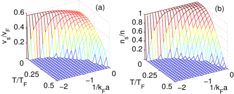
Figure 1: (Color online) (a) Superfluid sound velocity compared with Fermi velocity $v_{s}/v_{F}$ in superfluid regime. (b) Superfluid density compared with the total density $n_{s}/n$.

Fig. 1 shows the numerical plot of superfluid density and superfluid sound velocity with varying temperature and scattering length in the BCS regime.

V Damping

V.1 Approximate formulas of the damping rate

We start from the effective action, Eq. (32), for the superfluid phase field. Keeping $q$ small but finite when evaluating the coeffiencets $C_{1}$ and $C_{2}$ in Eq. (31), imaginary terms appear in Eq. (LABEL:eq:f1tof5), which corresponds to the damping of the collective modes. To get exact dispersion relation including damping for the superfluid phonons, one needs to self-consistently solve for poles of the effective action Eq. (32) of $\varphi$. However, in the regime where the damping is small, we can simplify the calculation.

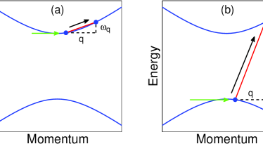
Figure 2: (Color online) Two separate damping channels. The blue curves are the fermionic quasi-particle spectrum. At $T=0$, the lower branch is fully occupied and the higher branch is empty. The green arrow is the incident phonon. The black arrow indicates the excitation of a fermionic quasi-particle. The red straight line is the linear spectrum of the phonon, where the slope is the sound velocity. The two black dashed lines are the changes of momentum and energy of fermionic quasi-particle, as indicated. (a) A phonon scatters an existing (by finite temperature) Fermi quasi-particle to a different state in the same energy branch. Such a process is known as Landau damping. This process can also happen in the lower branch at finite temperature, which is not shown here. (b) A phonon creates a quasi-particle and -hole pair across the lower and upper bands, equivalent to Cooper pair breaking in the representation of original particles.

The dispersion relationship is determined by setting the quadratic field term Eq. (32) to be zero. To evaluate the damping rate we apply a Wick rotation $i\omega_{n}=\omega_{0}-i\gamma$ as follows,

$$-C_{1}(\tilde{q})(\omega_{0}-i\gamma)^{2}+C_{2}(\tilde{q})\mathbf{q}^{2}=0,$$ (40)

$$\tilde{q}\equiv({\mathbf{q}},\ i\omega_{n}\rightarrow\omega_{0}+i0^{+})\,,$$

where $\omega_{0}$ is the oscillation frequency, or the real part of the phonon mode, and $\gamma$ is the damping rate. Although in principle, we should also keep $\gamma$ when applying the Wick rotation to the $\omega_{n}$’s in coefficients $f_{1},f_{2},f_{3}$, and $f_{4}$, for small damping it is sufficient to just apply $i\omega_{n}=\omega_{0}+i0^{+}$ for the coefficients to get the lowest order results. This approximation is similar to that adopted in the calculation for self-energy, for example, Ref. Liu (1997).

For the numerators in Eq. (LABEL:eq:f1tof5), we can still set $q=0$. The reason to do this is that the numerators are all real, and hence the small $q$ expansion gives only high order corrections to the zeroth order contribution. If we want only the leading order in the long wavelength expansion of the damping rate, the high order corrections in the numerators can be ignored, as we have checked.

Also, we can still use the results Eq. (LABEL:eq:coeffreal) obtained from last section for the real parts of $C_{1},C_{2},f_{1},f_{2},f_{3}$, and $f_{4}$, because we are not interested in the high order corrections to the real parts of coefficients, which just give higher order correction to the damping rate.

Adopting the above approximation, we can write $C_{1}=C_{1}^{\prime}+iC_{1}^{\prime\prime},C_{2}=C_{2}^{\prime}+iC_{2}^{\prime\prime},f_{1}=f_{1}^{\prime}+if_{1}^{\prime\prime}$ and so on, to find the poles of the effective action

$$(C_{1}^{\prime}+iC_{1}^{\prime\prime})(\omega_{0}-i\gamma)^{2}-(C_{2}^{\prime}+iC_{2}^{\prime\prime})\mathbf{q}^{2}=0\,.$$ (41)

Solving this equation gives the damping rate

$$\frac{\gamma}{\omega_{0}}=\frac{1}{2}\left(\frac{C_{1}^{\prime\prime}}{C_{1}^{\prime}}-\frac{C_{2}^{\prime\prime}}{C_{2}^{\prime}}\right)\,.$$ (42)

From Eq. (31), assuming that all the imaginary parts are small, we have

$$C_{1}^{\prime\prime} = f_{1}^{\prime\prime}+2\frac{f_{2}^{\prime}}{f_{3}^{\prime}}f_{2}^{\prime\prime}-\left(\frac{f_{2}^{\prime}}{f_{3}^{\prime}}\right)^{2}f_{3}^{\prime\prime}\,,$$

$$C_{2}^{\prime\prime} = f_{4}^{\prime\prime}\,.$$ (43)

After some calculation, we find that the imaginary parts of the coefficients $f^{\prime\prime}$’s can be separated into two channels $a$ and $b$, where in channel $a$

$$f_{1,a}^{\prime\prime} = \frac{\pi}{V}\sum_{\mathbf{k}}(1-\frac{\Delta_{0}^{2}}{E_{k}^{2}})\delta[\omega_{0}-(E_{k+q}-E_{k})](n_{k}-n_{k+q})\,,$$

$$f_{2,a}^{\prime\prime} = -\frac{\pi\Delta_{0}^{2}}{V}\sum_{\mathbf{k}}\frac{\xi_{k}}{E_{k}^{2}}\delta[\omega_{0}-(E_{k+q}-E_{k})](n_{k}-n_{k+q})\,,$$

$$f_{3,a}^{\prime\prime} = -\frac{\pi\Delta_{0}^{4}}{V}\sum_{\mathbf{k}}\frac{1}{E_{k}^{2}}\delta[\omega_{0}-(E_{k+q}-E_{k})](n_{k}-n_{k+q})\,,$$

$$f_{4,a}^{\prime\prime} = -\frac{\pi}{V}\sum_{\mathbf{k}}\frac{\mathbf{k}^{2}\cos^{2}\theta}{m_{a}^{2}}\delta[\omega_{0}-(E_{k+q}-E_{k})](n_{k}-n_{k+q})\,,$$

and in channel $b$

$$f_{1,b}^{\prime\prime} = \frac{\pi}{V}\sum_{\mathbf{k}}\frac{\Delta_{0}^{2}}{2E_{k}^{2}}\delta(\omega_{0}-E_{k}-E_{k+q})(1-n_{k}-n_{k+q})\,,$$

$$f_{2,b}^{\prime\prime} = \frac{\pi\Delta_{0}^{2}}{V}\sum_{\mathbf{k}}\frac{\xi_{k}}{2E_{k}^{2}}\delta(\omega_{0}-E_{k}-E_{k+q})(1-n_{k}-n_{k+q})\,,$$

$$f_{3,b}^{\prime\prime} = -\frac{\pi\Delta_{0}^{2}}{V}\sum_{\mathbf{k}}(\frac{1}{2}-\frac{\Delta_{0}^{2}}{2E_{k}^{2}})\delta(\omega_{0}-E_{k}-E_{k+q})\,,$$

$$\times(1-n_{k}-n_{k+q})\,,$$

$$f_{4,b}^{\prime\prime} = 0\,.$$

For the expressions above, we would like to remind the reader of the definitions of

$$E_{k}=\sqrt{\xi_{k}^{2}+\Delta^{2}}\quad\mbox{and}\quad n_{k}={1\over e^{\beta E_{k}}+1}.$$

The physical meaning of channel $a$ and $b$, as defined in the above expressions, is illustrated in Fig. 2. Channel $a$ (Fig. 2(a)) is the Landau damping. A (fermionic) quasi-particle absorbs or emits a superfluid phonon and becomes another quasi-particle state at a different momentum within the same energy band. In channel $b$ (Fig. 2(b)), a superfluid phonon excites a quasi-particle from the lower band to the upper band, creating a particle-hole pair excitation in the quasi-particle eigenvector basis, which corresponds to a Cooper pair breaking process in terms of original fermions. Both channels cause the superfluid phonons (collective exicitations of the superfluid state) to decay.

Before applying our theory to real experimental systems, let us discuss the properties of the damping in the $\omega_{0}\rightarrow 0$ limit (with $\omega_{0}/|\mathbf{q}|=v_{s}$ fixed) at low temperature, where channel $b$ vanishes. To satisfy the $\delta$ function in Eq. (LABEL:eq:imf1tof5a), we need to have

$$|\cos\theta|=\left|\frac{E_{k}mv_{s}}{\xi_{k}k}\right|\leq 1,$$ (46)

which is difficult to solve analytically.

We can still get some analytical properties if we combine the numerical and analytical analysis. At $1/k_{F}a=-0.45$ and $T/T_{F}<0.1$, numerical analysis shows that $k<{k_{\mu}}$ does not contribute to the integral. For $k>k_{\mu}$, we can substitute $k=k_{\mu}$ in Eq. (46), except for $\xi_{k}$, to get the range of $\xi_{k}$. We then apply a one-step iteration to get a more precise range for $\xi_{k}$. To satisfy Eq. (46), we need to have

$$\xi_{k} > \frac{\sqrt{\xi_{0}^{2}+\Delta^{2}}mv_{s}}{\sqrt{2m(\xi_{0}+\mu)}}\equiv\xi_{1},$$

$$\xi_{0} = \frac{\Delta mv_{s}}{k_{\mu}}.$$ (47)

The next step is to write

$$n_{k}-n_{k+q}$$ (48)

$$\approx \frac{\partial n_{k}}{\partial E_{k}}\cdot(E_{k}-E_{k+q})$$

$$= \beta\omega_{0}n_{k}(1-n_{k})$$

$$\approx \beta\omega_{0}e^{-\beta E_{k}}.$$

The second line comes from $\omega_{0}\ll T$ and the fourth line comes from $T\ll\Delta$. Also, numerical analysis shows that the contribution from $C_{1}^{\prime\prime}$ is much smaller than that from $C_{2}^{\prime\prime}$ in the above regime. In addition, at low temperature, $C_{2}^{\prime}\approx n/2m_{a}$ since the normal density is negligible. Taking all the above into account, we get

$$\frac{\gamma}{\omega_{0}}\approx\frac{3\pi}{4}\frac{v_{s}^{3}}{v_{f}^{3}}\frac{1}{T}\int_{E_{k}>\sqrt{\xi_{1}^{2}+\Delta^{2}}}dE_{k}\frac{E_{k}^{4}}{\xi_{k}^{4}}e^{-\beta E_{k}}.$$ (49)

The integral in Eq. (49) needs to be evaluated numerically in general cases. In the extremely low temperature, we can approximately treat $E_{k}^{4}/\xi_{k}^{4}$ in Eq. (49) as a constant and substitute in $\xi_{k}=\xi_{1}$, which gives

$$\frac{\gamma}{\omega_{0}}\approx\frac{3\pi}{4}\frac{v_{s}^{3}}{v_{f}^{3}}\frac{(\xi_{1}^{2}+\Delta^{2})^{2}}{\xi_{1}^{4}}e^{-\frac{\sqrt{\xi_{1}^{2}+\Delta^{2}}}{T}}.$$ (50)

An interesting feature of damping is that in Eq. (49) and (50), $\gamma/\omega_{0}$ is independent of $\omega_{0}$ when $\omega_{0}\ll T$. Therefore, we should observe the damping even in the $\omega_{0}\rightarrow 0$ limit in finite temperature. A physical understanding of this feature is that the damping from channel $a$ is the coupling between superfluid sound (phonon) and thermally excited Fermi quasi-particles, so that

$$\gamma \propto \int dkf(k,\Delta,\mu)(n_{k}-n_{k+q})$$ (51)

$$\propto \omega_{0}\int dkf(k,\Delta,\mu)\frac{dn_{k}}{dE_{k}},$$

where $f(k,\Delta,\mu)$ is an arbitrary function independent of $\omega_{0}$. This provides an experimental method to verify our theory, which will be discussed later.

In the following section, we will apply our theory to real experimental systems. We will focus on the regime of $\gamma/\omega_{0}\ll 1$ on the BCS side of the Feshbach resonance, where our approximations are quantitatively controlled.

V.2 Comparison with experiments

The above theory can be applied to real physical systems . We apply our method to the experimental configuration in Ref. Wright et al. (2007) and calculate the damping rate as function of both temperature and scattering length. The number of particles is $N=4\times 10^{5}$. The trapping frequencies are $\omega_{x}=2\pi\times 830\ \textrm{Hz}$, $\omega_{y}=2\pi\times 415\ \textrm{Hz}$ and $\omega_{z}=2\pi\times 22\ \textrm{Hz}$. Thus, $\bar{\omega}=(\omega_{x}\omega_{y}\omega_{z})^{1/3}=2\pi\times 196\ \textrm{Hz}$. Reading from Ref. Wright et al. (2007), the oscillation (phonon) frequency is $\omega_{0}\approx 2\pi\times 940\ \textrm{Hz}\approx 4.8~{}\bar{\omega}$. According to $\bar{\omega}/T_{F}=1/(3N)^{1/3}$, we get the ratio between the phonon energy and Fermi temperature

$$\frac{\omega_{0}}{T_{F}}=0.045.$$ (52)

From $\omega_{0}=v_{s}|\mathbf{q}|$ and $E_{F}=\frac{1}{2}v_{F}k_{F}$, we get

$$\frac{|\mathbf{q}|}{k_{F}}=\frac{1}{2}\frac{v_{F}}{v_{s}}\frac{\omega_{0}}{E_{F}}.$$

Since in most regime ${v_{F}}/(2v_{s})\sim O(1)$ as shown in Fig. 1, using Eq. (52) we conclude that $|\mathbf{q}|$ is also much smaller than the Fermi momentum $k_{F}$. Thus, our model, which requires $q$ to be small, can be applied to this physical system.

Figure 3: (Color online) Damping rate of collective excitations in superfluid regime showing dependence on $T/T_{F}$ and $1/k_{F}a$. When $T$ is close to $T_{c}$, the results from our approximation are no longer reliable since the damping rate $\gamma$ is already very large compared with $\omega_{0}$. This regime is indicated by the plateau. Also, when the system is no longer superfluid ($T>T_{c}$), our effective field theory does not apply, and the damping rate is then not plotted there.

Fig. 3 shows the numerical results of damping rate from channel $a$. It shows that the damping rate increases for higher temperature and smaller scattering amplitude $|a|$. In the superfluid regime, when $T$ is close to $T_{c}$, the damping rate $\gamma/\omega_{0}$ becomes big. When solving the equations for the damping rate in the preceding section, we assumed a small damping $\gamma$ compared with the oscillation frequency $\omega_{0}$, i.e., kept only the leading order in the perturbative expansion of $\gamma/\omega_{0}$. In the regime of big $\gamma/\omega_{0}$ where a significant correction is expected, our damping formula is no longer reliable. Thus, we use a plateau to indicate the regime of $\gamma/\omega_{0}>0.5$. Also, in the normal Fermi Liquid regime $T>T_{c}$ where our theory no longer applies, we keep the damping plot open with no data points shown, and will discuss this regime later.

We did not include channel $b$ when plotting Fig. 3. The reason is that we found that under the experimental condition Wright et al. (2007), the contribution to damping due to channel $b$ is much smaller than due to channel $a$. To investigate the features of channel $a$ and channel $b$ in more details, let us start from the relationship $\omega_{q}=v_{s}|\mathbf{q}|$. We focus in the regime of long wavelength and low temperature such that $k_{F}\gg|\mathbf{q}|$, and $T$ is not close to $T_{c}$. Thus $\Delta(T)$ is of the same order as $E_{F}$. In channel $a$, the first requirement is finite temperature, so that the upper (lower) band is populated by quasi-particles (quasi-holes) due to thermalization. This fact is enforced by the factor $(n_{k}-n_{k+q})$ in Eq. (LABEL:eq:imf1tof5a). The second requirement is energy conservation. The energy change of the fermionic quasi-particle after scattering with a phonon is as follows,

$$\delta E=E_{k+q}-E_{k}\approx\frac{\xi_{k}}{E_{k}}\frac{\mathbf{k\cdot q}}{m_{a}}\leq\frac{\xi_{k}}{E_{k}}\frac{|\mathbf{k}||\mathbf{q}|}{m_{a}}.$$ (53)

$\omega_{q}\approx\delta E$ is needed to satisfy the energy conservation. Therefore, we have

$$\omega_{q}=v_{s}|\mathbf{q}|\leq\frac{\xi_{k}}{E_{k}}\frac{|\mathbf{k}||\mathbf{q}|}{m_{a}}.$$ (54)

If $|\mathbf{k}|$ is too far away from $k_{F}$, both the finite-temperature occupation number and the density of states are greatly suppressed. Equivalently, the most effective scattering of phonons is from quasi-particle states around the upper (lower) band’s minimum (maximum). In addition, we have learned in Fig. 1 that $v_{s}$ does not exceed the order of $v_{F}$. As long as $|\mathbf{k}|$ is of the order $k_{F}$ or smaller, in principle, phonons of both large and small $v_{s}$ may excite fermionic quasi-particles in channel $a$. However, the condition Eq. (54) suggests that small $v_{s}$ is much more favored in channel $a$.

In channel $b$, the pair breaking process is allowed by the condition of occupation number at $T=0$ ($n_{k}=n_{k+q}=0$ in Eq. (LABEL:eq:imf1tof5b)). However, in this case,

$$\delta E=E_{k+q}+E_{k}\geq 2\Delta\,,$$ (55)

where the minimal value of $\delta E$ takes place for $k$ around $k_{F}$. Again, by energy conservation, $\omega_{q}\approx\delta E$ is required. Subsequently, we find the minimal condition required of the sound velocity $v_{s}$,

$$v_{s}\geq\frac{\Delta}{E_{k}}\frac{k_{F}}{|\mathbf{q}|}v_{F}.$$ (56)

As long as $\Delta$ is of the same order of $E_{F}$, and given that $k_{F}/|\mathbf{q}|$ is quite large, the condition Eq. (56) in turns requires that the sound velocity $v_{s}$ be much larger than the Fermi velocity $v_{F}$. In the superfluid phonon case, the condition $k_{F}\gg|\mathbf{q}|$ is satisfied, and when the temperature is still far away from $T_{c}$, channel $b$ is prohibited, since $v_{s}<v_{F}$ as shown in Fig. 1. Another way to understand that the damping channel $b$ is suppressed is to directly use energy conservation. Since $\omega_{q}\ll 2\Delta$, channel $b$ can not happen.

At finite temperature, channel $a$ becomes possible since some fermionic quasi-particles and holes are thermally created in the upper and lower band, respectively. They can scatter with superfluid phonons to cause decay. However, channel $b$ is still greatly suppressed as long as $w_{q}<2\Delta$.

In the experiment, Since $\omega_{0}/E_{F}\approx 0.04$, channel $b$ can happen only when when $\Delta(T)/E_{F}\approx 0.02$. From mean field analysis, near $1/k_{F}a\approx-0.5$, to satisfy $\Delta(T)/E_{F}\approx 0.02$, we need to have $T/T_{c}\approx 99.7\%$, which is very near the phase transition. However, according to Ref. Wright et al. (2007), the damping happens at $T\approx 0.6T_{c}$ near $1/k_{F}a\approx-0.5$, which is too low to let channel $b$ happen from our calculation. Even if one uses some theories including quantum fluctuation Fukushima et al. (2007), at $T\approx 0.6T_{c}$, $\Delta(T)/E_{F}$ is still much larger than $0.02$. Thus the damping peak should not correspond to the pair breaking channel $b$. As $T$ getting closer to $T_{c}$, channel $a$ will be more and more enhanced because of more and more thermally excited fermionic quasi-particles. When $\Delta(T)/E_{F}\approx 0.02$, channel $b$ also happens, while the damping from channel $a$ is already very large. It is not clear which channel dominates because $T$ near $T_{c}$ is outside the valid regime of our low energy effective field theory. It remains to be a challenge to formulate a quantum theory beyond the classical Boltzmann equation. Thus, our calculation just considered the contribution from channel $a$. We also double checked channel $b$ by numerical method and confirmed that the contribution from channel $b$ is zero for most regime.

There is another experimental evidence showing that why channel $b$ does not dominate. In the experiments varying the magnetic field Bartenstein et al. (2004); Altmeyer et al. (2007), if the pair breaking mechanism had dominated, one should also have observed very sharp peaks in these experiments. However, the damping rate changes relatively smoothly Bartenstein et al. (2004); Altmeyer et al. (2007), which means channel $a$ should be the reason for the smoothly increasing damping. Therefore, we expect the damping observed by changing the temperature Wright et al. (2007) to be due to channel $a$ too, since increasing the magnetic field at a finite temperature has the same effect as increasing the temperature at fixing magnetic field, both just reducing the gap. Nevertheless, the pair breaking channel $b$ is also possible to happen near the phase transition, but it is not necessarily dominating in contrary to what has been suggested.

The mechanism discussed here is different from the conventional acoustic attenuation process in solid-state superconductors, where channel $b$ overwhelms channel $a$ and $\omega_{q}\approx 2\Delta$. For the conventional case, $v_{s}$ is big, so that a relatively large phonon energy $\omega_{q}$ corresponds to a very small momentum $\mathbf{q}$. Channel $a$ is suppressed as $v_{s}$ is too big to satisfy the energy conservation condition (54). At the same time, a channel $b$ pair breaking process (Fig. 2(b)), associated with small momentum but large energy transfer from acoustic phonons to Fermi quasi-particles, may happen. The original fermion pair breaking process is the creation of a pair of particle and hole in the upper and lower branches of quasi-particle energy spectrum, respectively. A small $|\mathbf{q}|$ ensures that fermionic quasi-particles are created at the band extrema, which is known to result in a peak of damping rate, $\gamma\propto 1/\sqrt{\omega-2\Delta}$, due to the singularity of density of states. Therefore, the damping for large $v_{s}$ in traditional case is due to the pair breaking process (channel $b$).

We did not consider the fact that in the experiment, the fermionic gases are trapped and inhomogeneous in space. The above calculation is effective for gas at the center of the trap. On the edge of the trapped gas, by local density approximation, the effective density and Fermi energy is smaller than that of center, which means $\omega_{0}/E_{F}$ is larger and channel $b$ may happen in lower temperature (but still not very low yet). However, channel $a$ also happens on the edge since the above analysis still works for lower gas density on the edge, and the effect of channel $b$ is just to increase the damping rate, not giving a sudden peak.

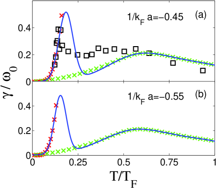
Figure 4: (Color online) Damping rate of collective excitations by interpolating results from our effective field theory in low temperature and the Boltzmann equation in high temperature. Red crosses are the prediction from our calculation in low temperature superfluid regime, and green crosses are from the Boltzmann equation. The blue solid line is the interpolation. The black squares are the experimental data of damping rgd . (a) $1/k_{F}a=-0.45$; (b) $1/k_{F}a=-0.55$. The first peak moves toward higher temperature when the system gets closer to the resonance (i.e., smaller $|1/k_{F}a|$).

In the regime $T>T_{c}$, where the system is no longer superfluid and our effective theory breaks down, the classical Boltzmann equation can be used to calculate the oscillation frequency and damping rate, as shown in Ref. Bruun and Smith (2007). As supplement to our main result above, we use the equation in Ref. Bruun and Smith (2007) to calculate the oscillation frequency. As mentioned there, the formulas did not take into account the effect of Pauli blocking, which means that the classical Boltzmann results are more valid at high temperatures. The calculation takes into account the trapping potential. At $1/k_{F}a=-0.45$, if we interpolate our theory in the low temperature superfluid regime with the results from Boltzmann equation in the high temperature Fermi liquid regime, two peaks by two different methods appear in Fig. 4, which agrees to the experimental results fairly well (cf. Fig. 2(b) in Ref. Wright et al. (2007)). Thus, we conclude that the first sharp peak observed in Ref. Wright et al. (2007) is due to the superfluid phonon and fermionic quasi-particle interaction, mostly through channel $a$ in Fig. 2(a). The second broad peak is given by the Boltzmann equation from Ref. Bruun and Smith (2007), which signals the hydrodynamic to collisionless transition. Our model further shows that the first damping peak moves toward higher temperature when the system gets closer to resonance (i.e., smaller $|1/k_{F}a|$), as one can see in the change from Fig. 4(b) to Fig. 4(a). This phenomenon was first reported in the experiments of Ref. Wright et al. (2007) (cf. Fig. 3 therein). In summary, our theory provides a consistent explanation for the experiments of damping.

According to our calculation, a damping due to phonon-fermion interaction should happen in the unitary limit. While this was not reported in the experiments of Ref. Wright et al. (2007), in the experiments of Ref. Kinast et al. (2005), the authors found that the damping rate of a Fermi gas at unitarity displays a weak peak immediately followed by a notch near transition as temperature increases. Such a damping notch is consistent with the dip of Fig. 4 that we propose here.

There are several reasons for the quantitative discrepancy between our calculation and the experiments. The most important thing is that our calculation is based on mean field results of $\Delta_{0}$ and $\mu$ from solving Eq. (13). Quantum fluctuations intend to destroy the superfluid phase, i.e., reduce the transition temperature $T_{c}$ below the mean field results. More reliable inputs for $\Delta_{0}$ and $\mu$ from calculation including quantum fluctuations Diener et al. (2008) will give a lower $T_{c}$, which will make our results better agree with experiments. Secondly, our calculation is based on Fermi gas in free space while in the experiments, the gas is always trapped. Thirdly, we used approximation to solve the damping. However, to be strict one needs to exactly solve for the poles. Also, $\omega_{0}$ is read from Ref. Wright et al. (2007) and treated as a constant in our work. That is just an approximation since $\omega_{0}$ is also changing slightly with temperature.

To verify our main conclusion that channel $a$ is the dominating process, we propose an experiment, which is to measure the damping rate $\gamma$ while varying the oscillation frequency $\omega_{0}$, and observe how $\gamma/\omega_{0}$ changes. This can be done by either increasing the particle number or reducing the trapping potential. If channel $b$, the pair breaking mechanism, is dominating, one should observe that the damping peak becomes increasingly narrower, and eventually is too narrow to be observable, as $\omega_{0}$ decreases. The reason is that the parameter regime to satisfy the energy conservation $\omega_{0}\approx 2\Delta$ diminishes with decreasing $\omega_{0}$, and eventually vanishes. On the other hand, if channel $a$, the Landau damping mechanism, is dominating, no matter how small $\omega_{0}$ is, as long as Eq. (46) is satisfied, the energy conservation law is always satisfied. Eventually $\gamma/\omega_{0}$ will be independent of $\omega_{0}$ in the limit of vanishing $\omega_{0}$ as discussed before in Eq. (51), and therefore the peak of damping $\gamma/\omega_{0}$ remains unchanged and should always be observable.

To summarize, we have studied the damping of collective modes for ultracold Fermi gases by effective field theory, and compared our results with experiments. By varying the temperature Wright et al. (2007) our theory predicts that one should find two peaks of damping. The first is a sharp peak due to the finite-temperature phonon-fermionic quasi-particle interaction, and the system changes from hydrodynamic superfluid to hydrodynamic Fermi liquid. The second is a broad peak due to the transition from the (collisional) hydrodynamic to collisionless Fermi liquid (see Fig. 4 in Ref. Wright et al. (2007)). In the experiment that varies the magnetic field Bartenstein et al. (2004); Altmeyer et al. (2007) but keeps temperature sufficiently low, one should see only the peak due to the phonon-fermionic quasi-particle interaction. After passing this peak, the system is already in the collisionless regime without the need of going across a collisionally hydrodynamic regime. Thus, there is no second broad peak.

References

- Nozières and Schmitt-Rink (1985) P. Nozières and S. Schmitt-Rink, J. Low Temp. Phys. 59, 195 (1985).
- Sá de Melo et al. (1993) C. A. R. Sá de Melo, M. Randeria, and J. R. Engelbrecht, Phys. Rev. Lett. 71, 3202 (1993).
- Giorgini et al. (2008) S. Giorgini, L. P. Pitaevskii, and S. Stringari, Rev. Mod. Phys. 80, 1215 (2008).
- O’Hara et al. (2002) K. M. O’Hara, S. L. Hemmer, M. E. Gehm, S. R. Granade, and J. E. Thomas, Science 298, 2179 (2002).
- Regal et al. (2004) C. A. Regal, M. Greiner, and D. S. Jin, Phys. Rev. Lett. 92, 040403 (2004).
- Zwierlein et al. (2004) M. W. Zwierlein, C. A. Stan, C. H. Schunck, S. M. F. Raupach, A. J. Kerman, and W. Ketterle, Phys. Rev. Lett. 92, 120403 (2004).
- Nascimbène et al. (2009) S. Nascimbène et al., Phys. Rev. Lett. 103, 170402 (2009).
- Bartenstein et al. (2004) M. Bartenstein et al., Phys. Rev. Lett. 92, 203201 (2004).
- Kinast et al. (2005) J. Kinast, A. Turlapov, and J. E. Thomas, Phys. Rev. Lett. 94, 170404 (2005).
- Joseph et al. (2007) J. Joseph et al., Phys. Rev. Lett. 98, 170401 (2007).
- Wright et al. (2007) M. J. Wright et al., Phys. Rev. Lett. 99, 150403 (2007).
- Altmeyer et al. (2007) A. Altmeyer et al., Phys. Rev. A 76, 033610 (2007).
- Stringari (2004) S. Stringari, Europhys. Lett. 65, 749 (2004).
- Heiselberg (2004) H. Heiselberg, Phys. Rev. Lett. 93, 040402 (2004).
- Hu et al. (2004) H. Hu, A. Minguzzi, X.-J. Liu, and M. P. Tosi, Phys. Rev. Lett. 93, 190403 (2004).
- Engelbrecht et al. (1997) J. R. Engelbrecht, M. Randeria, and C. A. R. Sáde Melo, Phys. Rev. B 55, 15153 (1997).
- Taylor et al. (2006) E. Taylor, A. Griffin, N. Fukushima, and Y. Ohashi, Phys. Rev. A 74, 063626 (2006).
- Fukushima et al. (2007) N. Fukushima, Y. Ohashi, E. Taylor, and A. Griffin, Phys. Rev. A 75, 033609 (2007).
- Diener et al. (2008) R. B. Diener, R. Sensarma, and M. Randeria, Phys. Rev. A 77, 023626 (2008).
- Holland et al. (2001) M. Holland, S. J. J. M. F. Kokkelmans, M. L. Chiofalo, and R. Walser, Phys. Rev. Lett. 87, 120406 (2001).
- Ohashi and Griffin (2002) Y. Ohashi and A. Griffin, Phys. Rev. Lett. 89, 130402 (2002).
- Ohashi and Griffin (2003) Y. Ohashi and A. Griffin, Phys. Rev. A 67, 063612 (2003).
- Vichi (2000) L. Vichi, J. Low Temp. Phys. 121, 177 (2000).
- Massignan et al. (2005) P. Massignan, G. M. Bruun, and H. Smith, Phys. Rev. A 71, 033607 (2005).
- Bruun and Smith (2007) G. M. Bruun and H. Smith, Phys. Rev. A 76, 045602 (2007).
- Riedl et al. (2008) S. Riedl et al., Phys. Rev. A 78, 053609 (2008).
- Urban and Schuck (2006) M. Urban and P. Schuck, Phys. Rev. A 73, 013621 (2006).
- Urban (2008) M. Urban, Phys. Rev. A 78, 053619 (2008).
- Liu (2006) W. V. Liu, Phys. Rev. Lett. 96, 080401 (2006).
- Mañes and Valle (2009) J. L. Mañes and M. A. Valle, Ann. Phys. 324, 1136 (2009).
- Schakel (2011) A. M. Schakel, Ann. Phys. 326, 193 (2011).
- Note (1) We treat the Jacobian as a constant using the same approximation in Ref. Diener et al. (2008); Paramekanti et al. (2000).
- Note (2) It means we adopt Gaussian approximation for the amplitude field and low energy expansion for the superfluid phase field.
- Note (3) To calculate , convergence factors are needed. See Ref. Diener et al. (2008).
- Taylor (2007) E. Taylor, Ph.D Thesis, University of Toronto (2007).
- Altland and Simons (2006) A. Altland and B. Simons, Condensed Matter Field Theory (Cambridge University Press, Cambridge, 2006).
- Note (4) In limit, we automatically neglect the bosonic fluctuation part in the normal density.
- Note (5) We used the mean field gap equation Eq. (10\@@italiccorr) to get . Including corrections due to quantum fluctuations may change its form. For detailed discussions on the effect of quantum fluctuations, see Ref. Diener et al. (2008); Taylor (2007).
- Combescot et al. (2006) R. Combescot, M. Y. Kagan, and S. Stringari, Phys. Rev. A 74, 042717 (2006).
- Liu (1997) W. V. Liu, Phys. Rev. Lett. 79, 4056 (1997).
- Note (6) One should notice that in experiments, the cold gases are trapped in anisotropic harmonic potentials. The parameters used here, i.e., the Fermi energy, chemical potential, etc., correspond to the values at the center of the trap.
- (42) R.G rimm (private communication).
- Paramekanti et al. (2000) A. Paramekanti, M. Randeria, T. V. Ramakrishnan, and S. S. Mandal, Phys. Rev. B 62, 6786 (2000).