On the critical temperatures of superconductors:
a quantum gravity approach

Andrea Gregori^†
Abstract
We consider superconductivity in the light of the quantum gravity theoretical framework introduced in [1]. In this framework, the degree of quantum delocalization depends on the geometry of the energy distribution along space. This results in a dependence of the critical temperature characterizing the transition to the superconducting phase on the complexity of the structure of a superconductor. We consider concrete examples, ranging from low to high temperature superconductors, and discuss how the critical temperature can be predicted once the quantum gravity effects are taken into account.

 ^†e-mail: agregori@libero.it

1 Introduction

Since its discovery in 1911 by Onnes superconductivity constituted one of the main domain of research of theoretical and applied physics. It cannot be explained within classical mechanics, and it has proven to be a test for the predictive power of quantum mechanics. Its fundamental theoretical explanation was given in 1957 by Bardeen, Cooper and Schrieffer [2], as due to the non-locality of electron wavefunctions which, under certain conditions, form bosonic pairs (Cooper’s pairs). At sufficiently low temperature, the latter collapse to a narrow energy width that, according to the Heisenberg Uncertainty Principle, implies a high delocalization in space. In the last decades superconductivity received new attention after the discovery of higher and higher temperature superconductors, opening the possibility of utilization of superconductors for practical purposes.

One aspect of high temperature superconductors that leaps to the eyes is the intriguing correlation that there seems to exist between critical temperature of transition to the superconducting phase, and the complexity of the lattice corresponding to a superconducting crystal . The grounds of a possible relation between lattice complexity and critical temperature remain however obscure. In the BCS theory, the critical temperature is related to the specific energies of the phonon excitations of the superconductor. In this way, it is possible to justify critical temperatures of some degrees Kelvin. Since the highest phonon frequency does not increase with an increase of the lattice length/complexity, this explanation seems to fail in the case of high temperatures. All these analyses are based on a quantum mechanical approach that does not consider gravity as a phenomenon whose quantum aspects should give a significant contribution. Indeed, it is common belief that gravity should play a negligible role in atomic and molecular phenomena, especially when one deals with objects at rest and not explicitly subjected to any kind of (unbalanced) gravitational force, either because the system is not accelerated, or, as in the case of a laboratory experiment on the earth, because the gravitational acceleration is negligible as compared to the strength of the other forces in the game. However, as a matter of fact lattice complexity means somehow geometric complexity of the mass/energy distribution along space (in this case a lattice element), and, according to General Relativity, talking of geometry of the energy concentration means somehow talking of gravity. Indeed, although irrelevant at the atomic scale from a classical point of view, gravity can play a role when quantized. In fact, quantization of gravity implies much more than just quantizing the graviton field: the latter is only the effect which is seen perturbatively. However, as is known, quantum gravity is not perturbatively stable as a quantum field theory. In this work, we consider it in the light of the non-perturbative quantum gravity framework proposed in Ref. [1]. Within this theoretical framework, once considered non-perturbatively, gravity can be shown to produce a deep modification of the whole quantum world, at any scale. In this work, we argue that quantum gravity plays a role also in the correlation between lattice complexity and critical temperature of superconductors.

In Ref. [1] I proposed a theoretical scenario in which the universe, namely, the whole detectable physical content of the universe, is, at any time, the result of the superposition of all possible configurations, i.e. distributions, assignments, of units of a degree of freedom, that we call ”energy”, along a target space of any possible dimension, that we call ”space of positions”. In its basic formulation, these spaces are discrete, so that these assignments are basically assignments of occupation numbers of cells, like binary strings of information, that tell whether a cell at a certain position in the target space bears a unit of energy or not. If we consider the set $\left\{\Psi\right\}_{E}$ consisting of all such configurations (distributions) at finite amount of total energy $E$, we can introduce an ordering through these sets, given by the amount of energy. As $\left\{\Psi\right\}_{E^{\prime}}\supseteq\left\{\Psi\right\}_{E}$ if $E^{\prime}\geq E$, the value of $E$ can be considered like a time coordinate, and the $E$-ordering through the sets $\left\{\Psi\right\}_{E}$ the time ordering through the history of the universe. All this sounds rather abstract, but, once these abstract configurations and their combinatorics are translated into the ordinary words and language of physics, they can be shown to produce the ”right” universe. The fact that what we observe is a superposition of configurations can be expressed by introducing a ”generating function” for the observables:

$${\cal Z}_{E}~{}=~{}\int{\cal D}\psi\,{\rm e}^{S}\,.$$ (1.1)

This is the sum over all the configurations $\psi$ at a given total energy $E$, weighted by their volume of occupation in the phase space of all the configurations $W(\psi)=\exp S(\psi)$ (the entropy $S$ is defined in the usual way, through $S\equiv\log W$). The sum 1.1 is taken over an infinite number of configurations, and, as such, in general diverges. The mean values of observables are however defined in a non-singular way, as:

$$\langle{\cal O}\rangle~{}\equiv~{}\frac{1}{\cal Z}\int{\cal D}\psi\,{\rm e}^{S}{\cal O}\,.$$ (1.2)

In this framework, causality is substituted by an evolution which, instead of being deterministic, is rather ”determined”: at any time, the average appearance of the universe is predominantly given by the configurations of highest entropy. This gives in the average a three-dimensional universe with the geometry of a three-sphere whose radius, after appropriate conversion of units, is $R\sim E$. One can show that the uncertainty introduced in neglecting more ”peripherical” configurations, namely, configurations of lower entropy, precisely corresponds to the Heisenberg’s position/momentum, or, better, time/energy, uncertainty (see Ref. [1]). The Heisenberg uncertainty principle can be considered as the ground statement of quantum mechanics, which can be viewed as the theoretical implementation of the Heisenberg’s uncertainty through a probabilistic wave-like description of physical phenomena. The way this uncertainty arises in this scenario leads to the interpretation of quantum mechanics as a practical way of parametrizing the undefinedness of the observables beyond a certain degree of approximation. Indeed, according to 1.2, the mean value of an observable receives contribution from an infinite number of configurations. In particular, in 1.2 are contained also an infinite number of configurations given by distributions of energy degrees of freedom along any space dimensionality, and, in general, escaping any interpretation in terms of the usual concepts of (smooth) geometry. The bound set by the Uncertainty Principle is here not simply a bound on the possibility of measuring certain quantities, but the “threshold” beyond which these quantities can not even be defined, because space, time, energy, momentum are only average, mean concepts that can be introduced only at a relatively large scale, averaging over an infinite number of configurations.

One can also show that in this scenario the maximal speed at which information propagates is the speed of expansion of the universe itself: $v_{\rm max}\propto dR/dE(=t)={\rm constant}$. This constant can be identified with the speed of light, and called $c$ (see Ref. [3]). Moreover, it can also be shown that the geometry of the distribution of energy is also the geometry of the trajectories of propagation. This theoretical framework describes therefore a quantum-relativistic scenario which, under appropriate limits to the continuum, can be well approximated by a string-theoretical description. The description in terms of string theory is however not a fundamental physical property in itself, but a representation useful for certain purposes, such as the determination of the physical content implicit in 1.1 in terms of spectrum of elementary particles, fundamental interactions, and the corresponding masses and couplings [4]. For the purposes of our present analysis, mapping to a string theoretical description is not necessary. What interests us here is that, in this theoretical framework, the Heisenberg’s uncertainty is the better and better satisfied as an equality by more and more “smooth” physical systems. The energy uncertainty is bounded from below by the uncertainty of the most “classical” configuration, the one of a three-sphere of radius $c\Delta t$, and energy content $\sim\left(M^{2}_{\rm Pl}c^{4}/\hbar\right)\Delta t$ (this is also the basic geometry of the universe itself [1, 4]): in this theoretical scenario we can say that the fact of being also gravity quantized reflects in the fact that the degree of non-classicity of a physical system turns out to depend on its“geometry”, intended in the general relativistic sense of space distribution of energy. More complex quantum systems show a higher degree of quantum delocalization.

Quite a few physical systems look almost like a three sphere with almost the energy density of a black-hole. But, as long as we look at sufficiently extended bodies with a big mass, uncertainties in position and momentum, even if not precisely at the “equality bound”, are nevertheless negligible. Things become more critical as we go to the atomic, and subatomic, scale. In that case, the difference between our theoretical framework and the usual approach becomes relevant. Superconductors are typical systems in which this phenomenon becomes critical and evident. These are materials which, although in themselves can be of huge extension, we are going to probe in their small scale properties. And, the more, by probes, the electrons, in a rather non-classical regime, such as the collective Cooper-pairs wave functions close to their ground energy. That is, where energy-momentum/time-position uncertainties play a relevant role, and where therefore quantum gravity effects show up more evidently. Apparently, this contradicts the popular idea that quantum gravity should become relevant only at the Planck scale. However, as it as discussed in [1] and [4], quantum gravity effects don’t show up only at the Planck scale, but also at a much lower scale. In particular, according to [4], also the masses of the elementary particles, and in particular the electron’s mass and the electroweak scale, find their natural explanation not within field theory, but as quantum gravity phenomena.

2 Quantum gravity and superconductors

The phenomenon of superconductivity is explained in its grounds as due to the formation of pairs of electrons, that, behaving thereby “collectively” as bosons, can fulfill a narrow band of energy obeying to Bose-Einstein statistics. In other words, there can be very many within such a narrow band, so to produce a non negligible electric current [2]. In the BCS argument essential for the occurring of this process is the existence of an attractive potential, attributed to the phononic response of the atoms of metal under charge displacement due to a motion of the electrons. This produces an energy gap $\Delta$, and it has been shown that at the critical temperature most of the electrons pairs lie in an energy range of order $\Delta$, at an energy which lies a gap $\Delta$ above the Fermi energy. This at least in the most simple formulation of the theory. More complicated structures of superconductors require modifications of this simple model, and eventually also weakens the existence of an energy gap as an essential feature of superconductivity, because there are conditions under which superconductivity exists even without an energy gap. We will not consider here the details of these model modifications and adjustments, which, as in any attempt to describe real, complex physical systems, are somehow unavoidable. For what interests our present discussion, it is important to consider that, whatever the derivation and the approximation introduced to reproduce a physical model can be, superconductivity remains related to the existence of a sufficient amount of electrons possessing a sufficient degree of non-locality. We can summarize this by introducing a “critical length” $\xi$, which, for reasons that will become clear in the following, does not necessarily coincide with the “coherence path” it is usually talked about in the literature about superconductivity. For the time being, let us just assume that, according to a certain mechanism, which can reasonably be the one of phonon response of the BCS approach, Cooper’s pairs do form and collect to a characteristic length higher than $\xi$ when the temperature is sufficiently low. It must be stressed that the distribution of electrons is not a mathematical step function. Step functions are useful approximations introduced in practical computations. In reality, it is a matter of statistics. Therefore, one should never forget that, at any temperature, there will be a certain amount of pairs with typical length below $\xi$, and a certain amount above $\xi$. The relative amounts are a matter of temperature. If we call $n$ the total number of electrons and $n_{S}$ the number of electrons which are paired and with typical length larger than $\xi$, we can define the critical temperature $T_{c}$ independently on the possible existence of an energy gap, just as the temperature at which $n_{S}/n\geq\left(n_{S}/n\right)_{0}$, $\left(n_{S}/n\right)_{0}$ being a certain well defined ratio, which does not need to be better specified. $\xi$ is therefore a mean quantity. In traditional quantum mechanics, where gravity is switched off, $\xi$ can only increase as a consequence of a higher localization in the space of momenta: $\langle\xi\rangle\sim\hbar/\Delta p\sim\hbar v_{F}/\Delta E$. In our quantum gravity scenario, $\langle\xi\rangle$ depends instead also on the complexity of the geometry of the system. We want to see how this comes about, and how, as a consequence, the critical temperature too will turn out to depend on the complexity of the geometry.

As discussed in Ref. [1], the uncertainty of the energy of a system during a time $\Delta t$ is:

$$\Delta E~{}\gtrsim~{}\frac{\Delta t}{\Delta S_{0}}\,,$$ (2.3)

where $\Delta S_{0}$ is the maximal possible entropy of a region created, “existing”, for a time $\Delta t$. The ordinary formulation of the Heisenberg’s uncertainty relation follows from expressing $\Delta S_{0}$ as $(\Delta t)^{2}$, the entropy of a black-hole of radius $\Delta t$ (in units for which we set $c$, the speed of light, to 1). This gives a lower bound on the energy uncertainty, and is almost satisfied as an equality only by configurations (i.e. physical systems corresponding to configurations) with a geometry/energy content close to that of a black hole. As we are going to discuss now, for configurations more remote, more “peripherical” in the phase space, the uncertainty will be higher.

Let us consider the sum 1.1. It describes a universe “on shell”; namely, the universe “as it is”. This means that there is no isolated system (particle or complex system of any kind), not embedded in its environment. In particular, there is no isolated system existing in a flat space. Not only the dominant configuration always contains the ground curvature of the universe, but any configuration $\psi$ involved in the sum 1.1 is a distribution of $E={\cal T}$ total energy degrees of freedom along a target space. Any configuration describes therefore a “whole universe”. If we want to consider just a particular system, we must make an abstraction, and 1) look at just a subset of the configurations contributing to 1.1, 2) for any configuration of this subset, we must restrict our attention to a subregion of space. There is here a subtlety, because, in general, $\psi$ does not describe a universe in three dimensions. As we said, this is true only for the dominant configurations. On the other hand, if it is true that the contribution of non-three dimensional, less entropic configurations is precisely what makes of the universe, and, in particular, of any subregion of it, a quantum system, it is also true that, in the concrete cases we want to consider here, a full bunch of these configurations, and precisely the most entropic ones, describe an energy distribution in a three dimensional space. Otherwise, we would not be able to talk of superconductors in the terms we are used to, namely, as well identified and (macroscopically) localized materials in a three-dimensional space. The physical systems we consider are therefore “at the border” between two descriptions: not anymore completely classical, but not even absolutely remote in the phase space, in order to completely escape the ordinary parameters of our perception of a three-dimensional space-time, and therefore of operational definition through a set of measurement and detection rules and experiments .

Let us concentrate our attention on just a small part the universe, a piece of superconducting material and, possibly, its close environment, with its atoms, electrons, magnetic fields etc., namely, all what constitutes our “experiment”. Let us call $E^{(sc)}$ the energy of this portion of the universe. Of course, $E^{(sc)}<E$, the total energy of the universe (indeed, obviously $E^{(sc)}\lll E$). Let us consider the bunch of configurations of the universe that contain our superconductor, $\left\{\psi^{(sc)}\right\}$. Of course, for what we said all the configurations contributing to 1.1 do contain also the portion of universe in which our superconductor is placed. However, what we want to do here is to select the subset of configurations that contribute in a non-trivial way to form up the shape of the superconductor, not just those that contribute, say, for the ground curvature of space.

When we measure the energy of our experiment, the quantity that we detect is a mean value of energy, $\langle E^{(sc)}\rangle$, defined as :

$$\langle E^{(sc)}\rangle~{}=~{}\frac{1}{\cal Z}\int_{\psi\in\left\{\psi^{(sc)}\right\}}{\cal D}\psi\;{\rm e}^{S}\,E^{(sc)}\,.$$ (2.4)

Let us consider how energy can be distributed in the space, in order to form up our experiment of mean energy $\langle E^{(sc)}\rangle$. According to 1.1, the more a configuration is remote in the phase space, the less it weights in the sum out of which we should compute the mean total energy of the experiment. Since in a finite region of space we can arrange only a finite amount of energy (we can put at most one unit of energy per each unit of space, where units of energy are measured in terms of Planck mass, units of space in terms of cells of Planck length size), to get a certain amount of mean total energy $\langle E^{(sc)}\rangle$ we must sum up over a larger and larger number of configurations. The larger and larger, the more and more remote the average configuration we want to describe. Moreover, since in a finite region of space we can arrange only a finite number of different configurations of energy, as we go further with the remoteness, to sum up to the same fixed amount of local energy $\langle E^{(sc)}\rangle$ we must include configurations $\psi^{(sc)}$, in which $E^{(sc)}$ is supported in larger and larger space regions. In terms of traditional quantum mechanics, this means that the wavefunctions are more and more spread out in space.

As discussed in [1] and [4], configurations can be classified according to the (finite) symmetry group of the distribution of energy degrees of freedom in the target space they correspond to. Their weight in 1.1 corresponds, by definition, to the number of times they occur in the phase space, in turn given by the number of equivalent ways they can be formed. The ratio of the weights in the phase space of two configurations can be expressed as:

$${W(\psi_{i})\over W(\psi_{j})}~{}=~{}{||G_{i}||\over||G_{j}||}\,,$$ (2.5)

where $G_{i}$ and $G_{j}$ are the symmetry groups, and $||G||$ indicates the volume of the group. This means that the more symmetric a configuration is, the higher is its weight in the phase space . If a configuration $\psi_{j}$ corresponds to a more broken symmetry group than a configuration $\psi_{i}$, it will be more remote, more “peripherical” in the phase space.

Let us introduce the concept of mean weight of our experiment, and of mean volume of the symmetry, or volume of the symmetry group of the mean configuration, through:

$$\langle W^{(sc)}\rangle~{}=~{}{1\over{\cal Z}}\int_{\psi\in\left\{\psi^{(sc)}\right\}}{\cal D}\psi\,{\rm e}^{S}\,,$$ (2.6)

and:

$${\langle||G^{(sc)}_{i}||\rangle\over\langle||G^{(sc)}_{j}||\rangle}~{}=~{}{\langle W^{(sc)}_{i}\rangle\over\langle W^{(sc)}_{j}\rangle}\,.$$ (2.7)

Accordingly, we define the mean configuration $\langle\psi^{(sc)}\rangle$ as the configuration for which:

$$W\left(\langle\psi^{(sc)}\rangle\right)~{}\stackrel{{\scriptstyle\rm def}}{{=}}~{}\langle W^{(sc)}\rangle\,.$$ (2.8)

Let us suppose we change the symmetry of the configuration of our superconductor, $\langle\psi^{(sc)}\rangle\to\langle\psi^{(sc)\prime}\rangle$, so that $||G^{(sc)}||\to||G^{(sc)\prime}||={1\over 2}||G^{(sc)}||$. In order to build up the same amount of energy $\langle E^{(sc)}\rangle$ we must consider configurations that distribute a higher amount of energy. How much more energy should we add, and how larger must be the space support? Approximately we must consider twice as much energy, and, in order to distribute it, at first sight we would say we need twice the volume. However, this second statement is not true. The point is that the maximal mean energy we can distribute along space, $\langle E\rangle$, goes linearly with the radius, not with the volume. To keep fixed the ratio of volumes of the symmetry groups, we must preserve the ratio of the entropies as compared with the maximal entropy, which is the one of a black hole of radius $\langle 2E\rangle$. Therefore, to maintain unchanged the value of $\langle E^{(sc)}\rangle$ and $||G^{(sc)\prime}||$, we need to consider distributions of twice as much energy along a region with twice the radius, not the volume. That is, energy goes linearly with the space length. Therefore, the spreading in space of wavefunctions is inversely proportional to the volume of the mean symmetry group:

$${\langle\Delta x\rangle\over\langle\Delta x\rangle^{\prime}}~{}=~{}{\langle||G^{(sc)\prime}||\rangle\over\langle||G^{(sc)}||\rangle}\,.$$ (2.9)

For any set of configurations with local symmetry group $G_{i}$, we may think of $G_{i}$ as the little group of symmetry surviving after quotienting a larger group $G$ through $h_{i}$. If we have two sets of configurations, $\psi_{i}$ and $\psi_{j}$, obtained by quotientation from the same initial group: $G_{i}=G/h_{i}$, $G_{j}=G/h_{j}$, we have:

$${W(\psi_{i})\over W(\psi_{j})}~{}=~{}{||h_{j}||\over||h_{i}||}\,.$$ (2.10)

Passing from the generic $\psi_{i}$, $\psi_{j}$ to $\psi^{(sc)}$, $\psi^{(sc)\prime}$, and introducing correspondingly $h^{(sc)}$, $h^{(sc)\prime}$ instead of $h_{i}$, $h_{j}$, we can write 2.9 as:

$${\langle\Delta x\rangle\over\langle\Delta x\rangle^{\prime}}~{}=~{}{\langle||h^{(sc)}||\rangle\over\langle||h^{(sc)\prime}||\rangle}\,.$$ (2.11)

Since we are working at fixed mean energy $\langle E^{(sc)}\rangle$, we are allowed to consider that, in both primed and unprimed situations, we have the same energy (or momentum) uncertainty. Indeed, as discussed in [1], the energy uncertainty is given by the contribution of the more peripherical configurations, with respect to those over which one takes the average in order to obtain the mean energy. Here, the energy uncertainty can be re-absorbed into a redefinition of mean volume of symmetry group, and therefore implicitly assumed to be fixed, in order to derive the scaling of the space (and time) spread out. Under these conditions, 2.11 tells us that $\langle||h^{(sc)}||\rangle$ can be viewed as an effective Planck constant:

$${\langle\Delta x\rangle\times\langle\Delta p\rangle\over\langle\Delta x\rangle^{\prime}\times\langle\Delta p\rangle}~{}=~{}{\langle||h^{(sc)}||\rangle\over\langle||h^{(sc)\prime}||\rangle}~{}\equiv~{}{h_{\rm eff}\over h_{\rm eff}^{\prime}}\,.$$ (2.12)

Up to an overall proportionality constant, that can be set to one, we can therefore write the quantum gravity version of the Heisenberg Uncertainty as:

$$\Delta x\Delta p~{}\geq~{}{1\over 2}\hbar_{\rm eff}\,,$$ (2.13)

where $\hbar_{\rm eff}\equiv h_{\rm eff}/2\pi$ is related to the symmetry of a configuration through 2.12, 2.11, 2.9 and 2.7. Since increasing $||h||$ corresponds to increasing the complexity of the configuration, things work as if the system would become less and less classical, more and more quantum mechanical, as the complexity of its structure increases.

We have identified the critical temperature of superconductivity $T_{c}$ as the temperature at which a well defined portion of electronic-bosonic states are delocalized at least as much as a critical length $\xi$. It is not necessary here to go into the details of the actual computation of $T_{c}$ within a specific model. It is enough to know that it is obtained by integrating over a statistical distribution of states, and that the latter is expressed in terms of weights depending on $E/kT$. Since everything depends on the ratio $E/T$, a rescaling of $E$ is compensated by a rescaling of the temperature $T$ while keeping fixed the ratio $E/T$. In other words, $T$ can be viewed as the unit of measure of $E$. To be concrete, let us consider once again our example of the two configurations characterized respectively by $||G^{(sc)}||$ and $||G^{(sc)\prime}||={1\over 2}||G^{(sc)}||$. In the primed case, the same delocalization in space as in the unprimed configuration corresponds to one-half the unprimed energy. Since both energies are effectively “measured” in units of $T$, instead of talking of half energy, we can speak of doubling the temperature. Coming back to the general case, consider that in 2.13 the effective Planck constant can be viewed both as setting the scale of length as compared to energy/momentum, or equivalently as setting the scale of energy/momentum as compared to space, and time. The relation 2.12 tells us therefore that, for more complex configurations, the same amount of electrons with space delocalization $\xi$ will be obtained at a higher critical temperature, according to:

$${T_{c}(i)\over T_{c}(j)}~{}=~{}{h_{\rm eff}(i)\over h_{\rm eff}(j)}\,.$$ (2.14)

In our theoretical framework, high critical temperatures show up as the consequence of the fact that, as expressed in 2.11, in superconductors with more complex geometrical structure, wavefunctions have a larger quantum uncertainty. In particular, keeping fixed all other parameters, they have a larger $\langle\xi\rangle$. Therefore, the condition $n_{S}/n\geq(n_{S}/n)_{0}$ is satisfied at higher temperature.

We stress that the considerations about the introduction of an effective, geometry-dependent Planck constant concern the delocalization of wave functions. Namely, the role the Planck constant plays in the Uncertainty Relations, $\Delta x\Delta p\geq h/4\pi$, $\Delta t\Delta E\geq h/4\pi$, not the value of this constant as a conversion unit between energy and time, or space and momentum, in contexts not related to the Uncertainty Relations . For instance, the energy levels as computed through the Schrödinger equation, or a set of Schrödinger equations, out of a classical description of effective potentials, are computed using the ground value of the Planck constant. On the other hand, once the energy eigenvalues of a system are known, a geometry-dependent Planck constant must be used, in order to obtain the effective spreading of wavefunctions in a geometrically complex quantum system. To this regard, a consideration about the size of characteristic lengths which are introduced in the physics of superconductors, such as the coherence lengths $\xi_{0}$, $\xi(T)$, and the London penetration length $\lambda$, is in order. One could have the impression that, as we are keeping fixed the critical delocalization of wavefunctions at the transition to the superconducting phase, the entire classification about what are type I and what type II superconductors, discriminated by the ratio $\lambda/\xi_{0}$, has to be reconsidered. Indeed, this is not true, and all the classical results to this regard go through unchanged in this scenario, because $\lambda$ contains in its definition the Planck constant. In other words, both lengths $\lambda$ and $\xi_{0}$ scale in the same way, and, as long as it is a matter of working with effective descriptions of superconductivity, such as for instance the Ginzburg-Landau effective theory, one can safely ignore rescalings, together with the grounds of a rescaling of the critical temperature.

3 Critical temperatures in various superconductors

We consider now various examples of superconductors, in order to see up to which extent an approach based on our effective quantum gravity scenario can be applied. The considerations of the previous section give us a clue on the role played by the geometry of a superconductor in determining its critical temperature. However, the detection of a regime of superconductivity is in general not a direct observation in itself: this regime is stated after observation of several properties, such as for instance the magnetic properties. Magnetic effects play a relevant role also in the generation of an effective resistivity. Therefore, superconducting regime, and critical temperature in particular, may be very sensitive to effects such as impurities, and in general doping effects aimed to pin magnetic vortices. Also external conditions such as pressure do play in general a significant role. All these conditions affect of course also the “geometry” of the physical configuration under experiment from the quantum gravity point of view, but quite often their most macroscopic effect reflects in the properties of superconductivity not as a consequence of a modified geometry, but as a consequence of a change in the dynamic magnetic properties or alike. Our investigation is therefore affected by a large amount of imprecision, and must be taken more as the indication of a tendency, than as a real precision test.

Low temperature superconductors are metals without a well defined “structure”. As mentioned in the introduction, in this case critical temperatures are, in their order of magnitude, well predicted within the BCS theory. Our concern will be with “structured” configurations, leading therefore to higher critical temperatures. On the other hand, according to our previous discussion, in our approach we do not obtain an absolute determination of critical temperatures, but only of their ratios, as a function of the ratios of geometries. For our analysis, we will therefore take as a reference point the low BCS temperatures. As a starting point we take mercury, which has a critical temperature around 4,2 ^oK. The reason why we consider this element instead of others is that it allows a simpler derivation of the ratio of weights, in the sense of 2.7, to the next material we want to consider, NbTi.

3.0.1 Hg $\to$ NbTi

As a first test of the idea let us consider NbTi, the first step above Hg in the list of the table of page 1. In first approximation, the structure of NbTi should correspond to a $Z_{2}$ breaking of the symmetry of Hg. This would be exactly true if Nb and Ti had the same mass and properties. Indeed, we can ideally consider the symmetry breaking as roughly occurring through the pattern:

$${}^{80}{\rm Hg}\,\stackrel{{\scriptstyle\sim Z_{2}}}{{\longrightarrow}}\,2\;^{41}{\rm Nb}\,\stackrel{{\scriptstyle\mathbbm{1}\times Z_{2}}}{{\longrightarrow}}\,^{41}{\rm Nb}\,+\,^{22}{\rm Ti}\,+\,^{22}{\rm Ti}////\,.$$ (3.16)

This is somehow in between $Z_{2}$ and $Z_{3}$: it has less symmetry than a $Z_{2}$, but more than a $Z_{3}$, in that Nb looks like twice Ti, so that it ideally comes from the recombination of a $Z_{2}$ symmetry subgroup out of a breaking into three Ti. The critical temperature of NbTi should therefore lie somehow between 2 and 3 times the one of Hg: $T_{c}({\rm NbTi})\sim(8,4+12,6)/2\sim 10,5^{\rm o}$K. Indeed, the observed critical temperature lies around 10 ^oK. Of course, our evaluation has to be taken only as a rough, indicative estimate.

In passing from Hg to NbTi we have introduced a “weighted” breaking of the Hg molecular symmetry. The weight is precisely the mass of the atoms into which the initial homogeneous energy distribution breaks. This is justified by the fact that, in our theoretical framework, the configurations $\psi$ in 1.1 and 1.2 are configurations of energy distributions along space. The size of the mass of a particle depends on the weight the configuration (or the set of configurations) in which this particle appears has in the phase space of all the configurations. In turn, the weight of a configuration depends on the symmetry of the energy distribution. Approximately, the latter is “measured” by the space gradient of energy: roughly speaking the higher is the density of energy gradient, the less homogeneous (= less symmetric) is the energy distribution. This can be understood as follows: let us consider a configuration, i.e. a particular distribution of energy along space, in its fundamental definition, as given in [1], namely, as a map from a discrete space to a discrete space. At any time we move one energy unit (unit energy cell in the language of [1]) from a position in the target space to a neighbouring one, we modify one symmetry group factor. If we move just one cell we increase (or decrease) the energy gradient by two units, and break (restore) one “elementary” group factor. If we move another unit, we increase (decrease) further the energy gradient by two units, and act once again on another elementary group factor, and so on. The amount of increase/decrease of the energy gradient is therefore proportional to the factor of increase/reduction of the symmetry group of the configuration. These considerations are true for the configurations $\psi$ entering in 1.1 and 1.2. However, owing to the properties of factorization of the phase space, and assuming that such a factorization is a good approximation when we want to “isolate” a local experiment such as those we are considering, we can transfer these global considerations also to the local description of superconductors. This implies neglecting the “extremely peripherical” configurations, anyway contributing for a minor correction, negligible for our present purposes. Therefore, instead of working with configurations as in 1.1 and 1.2, we work with “averaged” configurations as in 2.8, considering that everything outside the portion of universe we are testing remains unchanged. If we view configurations through an isomorphic representation in terms of symmetry groups:

$$\psi\,\leftrightarrow\,\prod_{j}G^{\psi}_{j}\,,$$ (3.17)

passing through the decomposition into an external and local part of the group:

$$\prod_{j}G^{\psi}_{j}\,=\,\left(\prod_{j}G^{\psi\,(ext)}_{j}\right)\times\prod_{j}G^{\psi\,(local)}_{j}\,,$$ (3.18)

it becomes clear that each configuration $\psi_{\alpha}$ can be factorized as:

$$\psi~{}=~{}\psi^{(ext)}\times\psi^{(local)}\,,$$ (3.19)

where “$local$” and “$ext$” precisely mean respectively the part of the configuration (or the corresponding symmetry group) describing the experiment (superconductor and related environment), and the rest of the universe. We can translate these considerations in terms of weights. Through the association:

$$\langle\psi^{(sc)}\rangle\,\longleftrightarrow\,\langle W^{(sc)}\rangle\,=\,\int_{\psi\in\{\psi^{(sc)}\}}{\cal D}\psi\,{\rm e}^{S}\left(\prod_{i}G^{\psi\,(ext)}_{i}\prod_{j}G^{\psi\,(local)}_{j}\right)\,,$$ (3.20)

we use the factorization 3.19 to first integrate over the external part of every configuration. As long as the portion of universe represented by our experiment is very small as compared to the rest of the universe, external and local part of configurations can be approximately treated as independent. Under this approximation, also the measure of integration can be factorized:

$${\cal D}\psi\,\longrightarrow\,{\cal D}\psi^{(ext)}\times{\cal D}\psi^{(local)}\,.$$ (3.21)

We can therefore write:

$$\frac{1}{\cal Z}\int_{\psi\in\{\psi^{(sc)}\}}{\cal D}\psi\,{\rm e}^{S}\left(\prod_{i}G^{\psi\,(ext)}_{i}\prod_{j}G^{\psi\,(local)}_{j}\right)\,\approx\,\left\langle\prod G^{(ext)}\right\rangle\times\langle G^{(local)}\rangle\,,$$ (3.22)

which allows to associate to $\langle\psi^{(sc)}\rangle$ a decomposition of weights:

$$\langle\psi^{(sc)}\rangle\,\to\,\langle W^{(sc)}\rangle\,\approx\,\langle W^{(ext)}\rangle\times\langle W^{(local)}\rangle\,.$$ (3.23)

This decomposition allows us to reduce the analysis of symmetries of configurations to just the crystal structure of our superconductors. The more, since superconductivity occurs as a property related to a characteristic length $\xi$, our considerations can be restricted to a region of this extension. In general, it is enough to look at a scale of order of the lattice length: the electron energy levels are given in terms of collective wave functions , and all quasi-particle energies are measured in terms of the lattice length $a$, which sets therefore the effective length/energy scale. In particular, when the energy gradient between neighbouring lattice periods is sufficiently “smooth”, it is possible to restrict the analysis to one lattice period. This is the case of the majority of the examples we are going to consider. With a certain degree of approximation, we can therefore write:

$$\langle W^{(local)}\rangle~{}~{}\propto~{}~{}\approx\,\int_{a}|\nabla E_{i}|_{a}\,.$$ (3.24)

3.23 allows us to write then:

$${\langle W^{(sc)}\rangle_{j}\over\langle W^{(sc)}\rangle_{i}}\,\approx\,{\int_{a_{i}}|\nabla E_{i}|_{a_{i}}\over\int_{a_{j}}|\nabla E_{j}|_{a_{j}}}\,\approx\,{h_{\rm eff}(i)\over h_{\rm eff}(j)}\,\approx\,{T_{c}(i)\over T_{c}(j)}\,.$$ (3.25)

Since we are talking of elements basically at rest, we can consider that the major contribution to the energy, determining the geometry of a configuration, comes from the rest energy, i.e. the mass. Therefore, to make the computation easier, instead of the integral of energy gradient we can consider the sum of the gradients of the mass distribution:

$$\int_{a}|\nabla_{x}E|_{a}~{}\approx~{}\sum_{k}^{(a)}|\Delta m^{(k)}|\,.$$ (3.26)

The ratios of critical temperatures between two such materials should approximately be:

$${T_{c}(i)\over T_{c}(j)}~{}\sim~{}{\sum_{k}^{(a_{i})}|\Delta m^{(k)}_{i}|\over\sum_{\ell}^{(a_{j})}|\Delta m^{(\ell)}_{i}|}\,.$$ (3.27)

This expression will allow us to investigate complex lattice structures. We stress that what matters is not simply the geometric lattice structure, with geometry intended as the space arrangement of atoms seen as massless geometrical solids, but the space distribution of energies, in the sense of general relativity. If in first approximation we neglect isotope effects, in the purpose of comparing ratios of gradients, instead of the mass, we may just consider the atomic number. We will now apply these considerations to the investigation of the next step in the table of page 1, Nb₃Sn.

3.0.2 Nb₃Sn

In the case of NbTi, the atomic numbers Nb = 41, Ti = 81 lead to:

$$\sum|\Delta m|=|41-81|=40~{}~{}~{}~{}~{}~{}~{}~{}({\rm NbTi})\,;$$ (3.28)

for Nb₃Sn, Nb = 41, Sn = 50 give:

$$\sum|\Delta m|=|41\times 3-50|=73~{}~{}~{}~{}~{}~{}~{}~{}({\rm Nb}_{3}{\rm Sn})\,;$$ (3.29)

The ratio of the sums of mass gradients of ${\rm Nb}_{3}{\rm Sn}$ to ${\rm NbTi}$ is therefore 1,825, that, from 3.27 and $T_{c}({\rm NbTi})\sim 10~{}^{\rm o}{\rm K}$ should lead to some $18\div 19$ ^oK for the Nb₃Sn critical temperature. The observed one is around 18 ^oK.

3.1 High temperature superconductors

Although more complex, high temperature superconductors are structured in layers, with a lattice structure that basically develops only along one coordinate. Their analysis is therefore, in first approximation, relatively simple, at least as long as one neglects the doping of certain sites with other elements. This introduces a further symmetry breaking that, in principle, leads to an enhancement of the estimated critical temperature. This operation may be considered somehow as a “built-in” ground effect, which underlies the properties of any one of these materials, and as such provides a systematic error, that can be observed in the general underestimating of the critical temperature. However, as doping varies from material to material, this further symmetry breaking cannot simply be “subtracted out” as a constant, universal effect: it introduces a further factor of uncertainty and approximation in our calculations. Our results should therefore be taken more for their capability to catch the main behaviour, than an attempt to really provide a fine evaluation of the exact critical temperature. As a matter of fact, our estimates fall anyway within an error of at most $15\%$ from the experimental observations.

3.1.1 LaOFeAs and SmOFeAs

For the iron-based superconductors we consider LaOFeAs and SmOFeAs. The crystal structure of LaOFeAs is arranged as a stack of layers in sequence (As) (Fe) (As) (La) (O) (La) etc. The one of SmOFeAs as a sequence of (As) (Fe) (As) (Sm) (O) (Sm) (see [6], [7] and [8]). The atomic numbers La = 57, O = 8, Fe = 26, As = 33 lead to:

$$\sum|\Delta m| = 2|m({\rm As})-m({\rm Fe})|+|m({\rm La})-m({\rm As})|+2|m({\rm La})-m({\rm O})|$$ (3.30)

$$+|m({\rm La})-m({\rm As})|$$

$$= 2|33-26|+|57-33|+2|57-8|+|57-33|=14+24+98+24=160$$

$$~{}~{}~{}~{}~{}({\rm LaOFeAs})\,;$$

Sm = 62, O = 8, Fe = 26, As = 33 lead to:

$$\sum|\Delta m| = 2|m({\rm As})-m({\rm Fe})|+|m({\rm Sm})-m({\rm As})|+2|m({\rm Sm})-m({\rm O})|$$ (3.31)

$$+|m({\rm Sm})-m({\rm As})|$$

$$= 2|33-26|+|62-33|+2|62-8|+|62-33|=14+29+108+29=180$$

$$~{}~{}~{}~{}~{}({\rm SmOFeAs})\,;$$

This gives as critical temperatures 42 and 47 ^oK respectively. The observed ones are 44 and 57 ^oK.

3.1.2 YBCO

We consider now the yttrium barium calcium copper oxide (YBCO) [9]. This material superconducts in its orthorhombic form. It is arranged as a stack of layers in sequence (Cu-O) (Ba-O) (Cu-O) (Y) (Cu-O) (Ba-O) (Cu-O). Differently from the previous examples, an evaluation of the mass gradients must here take into account also the fact that not only we have a gradient in passing from one layer to the neighbouring one, but also within each of the layers consisting of bonds of Ba and Cu with oxygen. In the planes presenting these bonds, it is not enough to just consider the gradient with the following plane: we must sum up also the mass gradient of the oxygen bond. On the other hand, in order to evaluate the overall gradient to be used in 3.27, it is not correct to sum up the absolute values of the “vertical” and the “horizontal” gradient. What counts for our purposes is the mean gradient contributed by each plane. We assume that, as in any propagation of errors, gradients in the two orthogonal axes sum up quadratically, as lengths of orthogonal vectors in a vector lattice. The overall gradient should approximately be given by the sum of the square roots of the quadratically propagated gradients of each layer, both in the “horizontal” and “vertical” directions. The evaluation of the mass gradient is complicated by the fact that, at the transition to the yttrium layer, oxygen couples both to copper and to yttrium, in an orthorhombic form. The crystal is therefore not structured in simple layers. In order to evaluate the mass gradient for the CuO₂-Y planes we make the approximation of attributing one oxygen atom to the copper layer, and one to yttrium. The expression of the sum of mass gradients is then :

$$\sum|\Delta m| = 2\times\left\{\sqrt{[(Cu+O)-(Ba+O)]^{2}+(Cu-O)^{2}}\right.$$ (3.32)

$$+\,\sqrt{[(Ba+O)-(Cu+O)^{2}]+(Ba-O)^{2}}$$

$$+\,\sqrt{[(Cu+O)-O]^{2}+(Cu-O)^{2}}$$

$$+\,\left.\sqrt{(O-Y)^{2}}\right\}\,.$$

Considering the atomic numbers Y = 39, Ba = 56, Cu = 29, O = 8, we have Cu + O = 37, Ba + O = 64, and Cu – O = 21, Ba – O = 48, and therefore:

$$\sum|\Delta m| = 2\times\left\{\sqrt{(37-64)^{2}+21^{2}}+\sqrt{(64-37)^{2}+48^{2}}+\sqrt{(37-8)^{2}+21^{2}}\right.$$ (3.33)

$$\,+\,\left.\sqrt{(8-39)^{2}}\right\}$$

$$\approx 2\times\left\{34,2+55,1+36+31\right\}~{}\approx~{}312~{}~{}~{}~{}~{}~{}~{}~{}~{}~{}~{}~{}~{}({\rm YBCO})\,.$$

Rescaling the temperature from the previous elements through 3.27, we obtain a critical temperature $T_{c}\approx 312/160\times 42\sim 82$ ^oK. If, in order to reduce the propagated error, instead of starting with the critical temperature of LaOFeAs as obtained through the series of rescalings from the metallic superconductors, we use as starting point its experimental value, 44 ^oK, we obtain for YBCO a critical temperature of $\sim 86$ ^oK. The experimental one is around $90\div 92$ ^oK.

The YBCO compound is part of a series, the so-called “123” superconductors, of similar critical temperatures, which differ by the substitution of yttrium with another element of the family of lanthanoids, including lanthanium. All these elements are heavier than yttrium, and we expect higher critical temperatures. This however is not always what happens. For instance, (Y_0.5Gd_0.5)Ba₂Cu₃O₇ with $T_{c}$ = 97 ^oK, (Y_0.5Tm_0.5)Ba₂Cu₃O₇ with 105 ^oK, and (Y_0.5Lu_0.5)Ba₂Cu₃O₇ with 107 ^oK present an increasing critical temperature, as expected from the increasing of mass of the elements that substitute the pure yttrium, and the further symmetry breaking due to the fact that yttrium is substituted by a mixture of elements, as indicated in the brackets. However, YbBa₂Cu₃O₇ has $T_{c}$ = 89 ^oK, and TmBa₂Cu₃O₇ has $T_{c}$ = 90 ^oK although Tm is lighter than Yb, and similarly GdBa₂Cu₃O₇ has $T_{c}$ = 94 ^oK, and NdBa₂Cu₃O₇ has $T_{c}$ = 96 ^oK, although Nd is lighter than Gd. A reason for this apparently odd behaviour could lie in the fact that the differences in atomic number are indeed very small, to the point that other effects play a non negligible role. A finer determination of the space layout of the energies and masses of these configurations would be in order.

There is another superconductor very similar to those of the YBCO series. It is YSr₂Cu₃O₇, which has a critical temperature $T_{c}$ = 62 ^oK. Strontium has atomic number 38, instead of the 56 of barium. In expression 3.33 we must therefore substitute Ba + O = 64 with 38 + 8 = 46, and Ba + O = 48 with Sr – O = 30. We have:

$$\sum|\Delta m| = 2\times\left\{\sqrt{(37-46)^{2}+21^{2}}+\sqrt{(46-37)^{2}+30^{2}}+\sqrt{(37-8)^{2}+21^{2}}\right.$$ (3.34)

$$\,+\,\left.\sqrt{(8-39)^{2}}\right\}$$

$$\approx 2\times\left\{22,9+31,3+36+31\right\}~{}\approx~{}242,4~{}~{}~{}~{}~{}~{}~{}~{}~{}~{}~{}~{}~{}({\rm YSrCCO})\,.$$

Rescaling from YBCO, we obtain a critical temperature of $63\div 64$ ^oK, in substantial agreement with the experiments.

3.1.3 BSCCO

We consider now the bismuth-strontium-calcium-copper-oxide superconductors (BSCCO) [10]: Bi2212 (Bi₂Sr₂CaCu₂O₂) and Bi2223 (Bi₂Sr₂Ca₂Cu₃O₁₀). The lattice structure of the Bi2212 form is a stack of the following layers: (Bi-O) (Sr-O) (Cu-O₂) (Ca) (Cu-O₂) (Sr-O) (Bi-O) (Bi-O) (Sr-O) (Cu-O₂) (Ca) (Cu-O₂) (Sr-O) (Bi-O). The Bi2223 is similar, with one more (Ca) (Cu-O₂) layer. As for YBCO, here too we must propagate both the “horizontal” and the “vertical” gradients. In this case the horizontal bonds are those of Bi, Sr and Cu with oxygen. For the Bi2212 form, we need therefore BiO = 83+8 = 91, SrO = 38+8=46, Ca = 20, CuO₂ = 29+16=45 and Bi–O = 75, Sr–O =30, Cu–O = 21, to give:

$$\sum|\Delta m| = 2\times\left\{\sqrt{[(Bi+O)-(Sr+O)]^{2}+(Bi-O)^{2}}\right.$$ (3.35)

$$+\,\sqrt{[(Cu+2O)-(Sr+O)]^{2}+(Sr-O)^{2}}$$

$$+\,\sqrt{[(Ca)-(Cu+2O)]^{2}+[(Cu-O)+(Cu-O)]^{2}}$$

$$= 2\times\left\{\sqrt{(91-46)^{2}+75^{2}}+\sqrt{(45-46)^{2}+30^{2}}+\sqrt{(20-45)^{2}+(21+21)^{2}}\right\}$$

$$\approx 2\times\left\{87,5+30+49\right\}~{}\approx~{}332~{}~{}~{}~{}~{}~{}~{}~{}~{}~{}~{}~{}~{}({\rm Bi2212})\,.$$

Rescaling the temperature from LaOFeAs through 3.27 we obtain a critical temperature $T_{c}\approx 332/160\times 42\sim 87$ ^oK. Starting from the experimental value, 44 ^oK, in order to reduce the propagated error, we obtain for the Bi2212 a critical temperature of $\sim 91$ ^oK, closer to the experimental one (92 ^oK).

The structure of Bi2223 is very similar to the one of Bi2212, with just the difference of a Ca, CuO₂ layer-pair in each half-lattice block. In order to obtain the mass gradient of Bi2223 we must therefore just correct the former evaluation by adding an amount $|m({\rm Ca})-m({\rm CuO}_{2})|+\sqrt{[m({\rm Ca})-m({\rm CuO}_{2})]^{2}+[2|m({\rm Cu})-m({\rm O})|]^{2}}$:

$$\sum|\Delta m| = \sum|\Delta m|({\rm Bi}(2212))+|20-45|+\sqrt{(20-45)^{2}+(21+21)^{2}}$$ (3.36)

$$= 332+74~{}=~{}406~{}~{}~{}~{}~{}~{}~{}~{}~{}~{}~{}~{}~{}~{}~{}~{}~{}~{}~{}({\rm Bi2223})\,,$$

corresponding to a temperature of $406/160\times 42=107$ ^oK ($\sim 111$ ^oK if we start from the experimental 44 ^oK for the critical temperature of LaOFeAs). The experimental value is around 110 ^oK.

3.2 The Tl-Ba-Ca-Cu-O superconductor

3.2.1 Tl₂Ba₂CuO₆ (Tl-2201)

The stacking sequence is as follows: (Tl-O) (Ba-O) (Cu-O₂) (Ba-O) (Tl-O) , and the expression of the mass gradient sum is:

$$\sum|\Delta m| = \sqrt{(Tl-O)^{2}+[(Tl+O)-(Ba+O)]^{2}}$$ (3.37)

$$+ \sqrt{[(Ba+O)-(Cu+O+O)]^{2}+(Ba-O)^{2}}$$

$$+ \sqrt{(Cu-O)^{2}+(Cu-O)^{2}+[(Cu+O+O)-(Ba+O)]^{2}}$$

$$+ \sqrt{[(Ba+O)-(Tl+O)]^{2}+(Ba-O)^{2}}$$

$$+ \sqrt{(Tl-O)^{2}+[(Tl+O)-(Tl+O)]^{2}}\,.$$

From the atomic numbers Tl = 81, Ba = 56, Cu = 29 and O = 8 we derive (Tl-O) = 73, (Tl + O) = 89, (Ba–O) = 48, (Ba + O) = 64, (Cu–O–O) = 21, and (Cu+O+O) = 45. Plugging these values into the gradient sum expression, we obtain:

$$\sum|\Delta m| = \sqrt{73^{2}+(89-64)^{2}}$$ (3.38)

$$+ \sqrt{(64-45)^{2}+48^{2}}$$

$$+ \sqrt{2\times 21^{2}+(45-64)^{2}}$$

$$+ \sqrt{(64-89)^{2}+48^{2}}\,+\,73$$

$$= 291\,.$$

Rescaling now from LaOFeAs, expression 3.30, and using once again the 44 ^oK of the experimental temperature, we obtain $(291/160)\times 44=80$ ^oK (had we used our calculated 42 ^oK for LaOFeAs, we would have obtained $\sim 76,5$ ^oK). The experimental critical temperature is around 80 ^oK.

3.2.2 Tl₂Ba₂CaCu₂O₈ (Tl-2212)

In this crystal there are two Cu-O-O layers with a Ca layer in between, with stacking sequence (Tl-O) (Ba-O) (Cu-O₂) (Ca) (Cu-O₂) (Ba-O) (Tl-O). In order to obtain the mass-gradient sum we have just to add to the previous computation a module:

$$\sqrt{[(Cu+O+O)-Ca]^{2}+(Cu-O)^{2}+(Cu-O)^{2}}\,+\,\sqrt{[(Cu+O+O)-Ca]^{2}}\,.$$ (3.39)

Considering that the atomic number of Ca is 20, this means an amount:

$$\sqrt{25^{2}+2\times 21^{2}}\,+\,25~{}=~{}64\,.$$ (3.40)

This gives a sum $291+64=355$, leading to a critical temperature of around 98 ^oK. The experimental one is around 108 ^oK.

3.2.3 Tl₂Ba₂Ca₂Cu₃O₁₀ (Tl-2223)

In this crystal there are three CuO₂ layers enclosing one Ca layer between each of them. That means, one more [(CU-O-O) Ca] module as compared to Tl₂Ba₂CaCu₂O₈. We obtain therefore a value of mass gradient sum $355+64=419$, leading to a critical temperature of 115 ^oK. The experimental one is 125 ^oK.

Both in this and in the previous superconductor we obtain slightly underestimated values of critical temperature. On the other hand, the ratio of the two critical temperatures we obtain, namely, $115/98$, is in better agreement with the ratio of the experimental values. Indeed, it gives a slight overestimate, which partially compensates the underestimate of the first temperature. From a qualitative point of view, these under/over-estimates can be understood as follows: when a Ca layer is added to the Tl₂Ba₂CuO₆ structure, the symmetry of the configuration of a stack of “(X-O)” layers gets further broken, because the Ca layer does not contain an oxygen bond. Not taking this into account leads to an underestimate of the increase in critical temperature. On the other hand, when a further identical layer is added, there is a partial restoration of symmetry, which implies a reduction in the increase of critical temperature, thereby our over-estimation. This effect becomes more relevant in more complicated configurations: in Tl-based superconductors, the value of $T_{c}$ decreases after four CuO₂ layers in TlBa₂Ca_n-1Cu_nO_2n+3, and in the Tl₂Ba₂Ca_n-1Cu_nO_2n+4 compound it decreases after three CuO₂ layers [14].

3.3 Comparing within families

Superconductivity is detected through investigation of the magnetic properties of materials. In particular, for what concerns high-temperature superconductors, pinning of magnetic flux through impurities plays a significant role, not only in reducing the effective resistance, and therefore affecting the conditions for the detection of a regime recognizable as the one of superconductivity, but, in the light of our analysis, also because it decreases the symmetry of the configuration. Also pressure plays a relevant role, because high pressures correspond to more remote configurations, and are expected to lead to higher critical temperatures (a fact that corresponds to the experimental observation). It is therefore rather difficult to give a correct quantitative account of the superconducting properties and the critical temperatures of all superconducting materials, and impossible to do it only in terms of comparison of average mass gradients referring to a single material taken as a universal starting point. In several cases, the best we can do is comparing critical temperatures within “families” of materials, which are assumed to share common properties, so that the change in the lattice structure taken into account by our evaluation of mass gradients can be considered as the only relevant variable and effective term of comparison.

3.3.1 Hg-Ba-Ca-Cu-O superconductor

An example of this kind of difficulties is provided by the Hg-series (Hg-1201, Hg-1212, Hg-1223  [15]). In principle, it is analogous to the series in which mercury is substituted by thallium (the Tl-series: Tl-1201, Tl, 1212, Tl-1223), but, while the critical temperature of Tl-1201 is lower than 10 ^oK, the one of the analogous compound made with Hg (one position lower in the atomic number scale) is around 94 ^oK. Both these numbers escape the predictions we can make with our simple mass-gradient arguments, applied using mercury as starting point. Indeed the Hg-1201 material is a critical example in which doping plays crucial role, whose details are still controversial. As reported in [16], depending on the amount of doping, this cuprate can superconduct or not, with a range of critical temperatures spanning the whole spectrum from zero to the maximal value. The critical temperature has proven to be also very sensitive to pressure [17]. In this case, the best we can do is to compare critical temperatures assuming comparable doping/flux pinning conditions. Assuming that, for instance, the highest critical temperature within the Hg-1201, 1212, 1223 series are obtained with a similar amount of such “external” inputs, we can expect to be able to give a reasonably good estimate of the ratios of critical temperatures within the Hg series. An illustration of the crystal structure of HgBa₂CuO₄ (Hg-1201, $T_{c}$ = 94 ^oK), HgBa₂CaCu₂O₆ (Hg-1212, $T_{c}$ = 128 ^oK) and HgBa₂Ca₂Cu₃O₈ (Hg-1223, $T_{c}$ = 134 ^oK) can be found in [13]. Computing the ratios of temperatures along the same line as in the previous examples, we obtain

$${T_{c}(Hg-1223)\over T_{c}(Hg-1212)} \sim 1,23\,,$$

$${T_{c}(Hg-1212)\over T_{c}(Hg-1201)} \sim 1,3\,,$$

$$\left({T_{c}(Hg-1223)\over T_{c}(Hg-1201)}\right. \sim \left.1,59\begin{array}[]{c}\mbox{}\\ \mbox{}\end{array}\right)\,,$$ (3.43)

to be compared with the ratios of the experimental ones, namely $1,05$, $1,36$, and $1,43$ for the ($1223\big{/}1201$) ratio. They show a similar situation of underestimate for the ratio of the lower pair of temperatures, and overestimate for the ratio of the third to the second one, as in the case of the thallium compound discussed above. Taking this into account, the ratios we find are not far from the experimental ones (the absolute determination of the temperature fails in this case to give a correct prediction, in that it would tell that both the thallium and the mercury -1201, -1212, -1223 series should have the same critical temperatures). This suggests that, keeping fixed all other conditions, the argument based on the evaluation of symmetry properties of the mass/energy configurations makes sense, although in some cases it is too simplified, and not sufficient to determine the overall conditions producing the particular state of a material which is detected as a regime of superconductivity.

A comparison restricted to elements belonging to the same family is our way of proceeding also in the case of higher temperature superconductors. Indeed, when passing to higher-$T_{c}$ superconductors, and therefore to higher complexity of the lattice structure, a thorough analysis of the details of any part of the lattice block becomes the more and more difficult. On the other hand, in first approximation a detailed knowledge of the full lattice structure is not even necessary. The materials we are going to consider can be grouped in “families”, whose elements share part of the lattice structure, and differ by the structure of just one (or some) of the lattice blocks. In this way, it is possible to perform a partial analysis, by comparing the critical temperatures among the members of each family. As the whole structure becomes longer and longer, it becomes smaller the error we introduce in weighting the various blocks according to their average length, thereby neglecting the details of the single mass gradients within common blocks. The difference from one material to the neighbouring one within a family usually consists in the substitution of some atomic elements, or in the addition of further replicas of already present layers. The mass differences introduced by these changes will be dealt with as a “second order” perturbation:

$${T^{\prime}_{c}\over T_{c}}~{}=~{}{T_{c}+\delta T_{c}\over{\rm T}_{c}}~{}=~{}1+{\delta T_{c}\over T_{c}}~{}\approx~{}1+\delta|(\nabla M)|_{\rm extra~{}block}\Big{/}\sum|\nabla M|\,.$$ (3.44)

3.3.2 The SnBaCaCuO to (TlBa)BaCaCuO family.

• From 160 ^oK (Sn₃Ba₄Ca₂Cu₇O_ν) to 200 ^oK (Sn₆Ba₄Ca₂Cu₁₀O_ν).

  The lattice structure of Sn₃Ba₄Ca₂Cu₇O_y consists of a stack of (Ca) (CuO_x) [ (Ba) (CuO_y) (Ba) ] (CuO_x) (Ca) (CuO_x) [ (Ba) (Sn-O) (Cu) (Sn-O) (Cu) (Sn-O) (Ba) ] (CuO_x) , where in the first square bracket we indicate the light part of the lattice, in the second the heavy part, and (CuO_x), (CuO_y) indicate copper oxide layers. Here and in the following we use this notation to indicate, in general, (CuO₃) and (CuO₂) layers respectively . The lattice structure of Sn₆Ba₄Ca₂Cu₁₀O_ν is obtained by doubling the “heavy” part of the lattice of Sn₃Ba₄Ca₂Cu₇O_ν. The structure of this superconductor corresponds therefore to that of Sn₃Ba₄Ca₂Cu₇O_ν, with the duplication of an entire lattice block. For the evaluation of the critical temperature we assume that, owing to the high number of lattice elements/layers, in first approximation we can consider the geometry of the blocks structure as prevailing over the fine structure of energy gradients, which distinguishes between light and heavy part of the lattice. That means, in first instance we deal with the blocks as if all lattice layers were equal, something that in the average is not far from the truth, and implies an error that becomes smaller and smaller as we go on with an increasing length of the crystal structure. Since the “replica” of the lattice block we add to obtain this superconductor corresponds to around 1/4 of the whole structure, we expect some 25% of increase in $T_{c}$ from the one above, corresponding to an increase from 160 to 200 ^oK .

• 212 ^oK: (Sn₅In)Ba₄Ca₂Cu₁₀O_ν

  The lattice structure consists of a stack of the following layers: (Ca) (CuO_x) [ (Ba) (CuO₂) (Ba) ] (CuO_x) (Ca) (CuO_x) [ (Ba) (Sn,In-O) (Cu) (Sn,In-O) (Cu) (Sn,In-O) (Cu) (Sn,In-O) (Cu) (Sn,In-O) (Cu) (Sn,In-O) (Ba) ] (CuO_x). We expect a higher $T_{c}$ than the crystal of above (200 ^oK), as a consequence of the lower symmetry, now broken by the substitution of a tin atom with indium. This corresponds to a breaking of more or less one out of $18\div 20$ lattice layers, i.e. a $\sim 5\div 6\%$ of the total. Since the mass difference between Sn and In is of much lower order, in first approximation the increase of the critical temperature should be mainly determined by the symmetry breaking among different lattice layers, and therefore be of order $\sim 5\div 6\%$. This gives indeed some 210-212 ^oK, as is observed.

  The mass difference between Sn and In plays a role as a second order effect, that can be observed in the smaller variation of the critical temperature after a change of the (Sn₅In) structure into (Sn₄In₂). The (Sn₅In) compound should superconduct at a higher temperature than (Sn₄In₂), where there is a partial reconstruction of a higher symmetry within indium planes. Experimentally, one observes 212 ^oK for the first, and 208 ^oK for the second. Also in this case, an evaluation, even approximate, is rather difficult, because the naive value of 5/4 one would suppose (20% increase in the temperature) must be ”tempered” by the fact that Sn and In weight almost the same. Their relative mass difference is 1/50, and this would mean a symmetry breaking of about 2%, indeed corresponding to the order of change in the observed $T_{c}$.

• 218 ^oK: (Sn₅In)Ba₄Ca₂Cu₁₁O_ν

  The lattice structure is similar to the one of (Sn₅In)Ba₄Ca₂Cu₁₀O_ν but contains one extra Cu in the light part of the lattice: (Ca) (CuO_x) [ (Ba) (Cu₂O_y) (Ba) ] (CuO_x) (Ca) (CuO_x) [ (Ba) (Sn,In-O) (Cu) (Sn,In-O) (Cu) (Sn,In-O) (Cu) (Sn,In-O) (Cu) (Sn,In-O) (Cu) (Sn,In-O) (Ba) ] (CuO_x). Adding a copper atom breaks part of the symmetry, thereby increasing $T_{c}$. As this occurs in one of the some 22 lattice ”stairs”, we would expect this to produce a correction of about $\sim$1/22 = 4,5% of $T_{c}$. This would mean some 9 ^oK. However, in this estimate we don’t consider finer corrections obtained by taking into account mass gradients. In practice, the breaking of symmetry is softened by the fact that there is a partial restoration of symmetry due to the fact that we are adding one more atom in a layer made of atoms of the same element. Indeed, the correction which is experimentally observed seems to be around 6 ^oK, indicating a slightly lower symmetry breaking than in our rough estimate.

• 233 ^oK: Tl₅Ba₄Ca₂Cu₁₁O_ν

  The lattice structure is given by the following stack: (Ca) (CuO_x) [ (Ba) (Cu₂O_y) (Ba)] (CuO_x) (Ca) (CuO_x) [ (Ba) (Tl-O) (Cu) (Tl-O) (Cu) (Tl-O) (Cu) (Tl-O) (Cu) (Tl-O) (Ba) ] (CuO_x). The heavy part of the lattice is similar to the one of the previous cuprate, with the suppression of the indium layer, and the substitution of tin atoms with thallium. In order to compare critical temperatures, let us compute the mass gradient sums corresponding to this part of the lattice for both these materials. They correspond to the stacking sequences (Ba) (Sn-O) (CuO) (Sn-O) (Cu) (Sn-O) (Cu) (Sn-O) (Cu) (Sn-O) (Cu) (Sn-O) (Ba) and (Ba) (Tl-O) (Cu) (Tl-O) (Cu) (Tl-O) (Cu) (Tl-O) (Cu) (Tl-O) (Ba) respectively. In the Sn sequence, one of the six tin atoms is substituted by an indium atom. Since the atomic numbers are respectively In = 49 and Sn = 50, in first approximation we neglect the slight asymmetry introduced by the (5 Sn)/In alternance. The mass gradient sums are:

  $$\sum|\Delta m| = |Ba-(Tl+O)|$$ (3.45)

  $$\,+\,4\times\left\{\sqrt{(Tl-O)^{2}+[(Tl+O)-Cu]^{2}}\,+\,|Cu-(Tl+O)|\right\}$$

  $$\,+\,\sqrt{(Tl-O)^{2}+[(Tl+O)-Ba]^{2}}\,,$$

  and, neglecting the difference between Sn and In:

  $$\sum|\Delta m| = |Ba-(Sn+O)|$$ (3.46)

  $$\,+\,5\times\left\{\sqrt{(Sn-O)^{2}+[(Sn+O)-Cu]^{2}}\,+\,|Cu-(Sn+O)|\right\}$$

  $$\,+\,\sqrt{(Sn-O)^{2}+[(Sn+O)-Ba]^{2}}\,.$$

  Inserting the atomic numbers Ba = 56, Tl = 81, Cu = 29, O = 8 and Sn = 50 we obtain:

  $$\sum|\Delta m|({\rm Tl}_{5}) = |56-89|\,+\,4\left\{\times\sqrt{73^{2}+(89-29)^{2}}\,+\,|29-89|\right\}$$ (3.47)

  $$\,+\,\sqrt{73^{2}+(89-56)^{2}}$$

  $$= \,33+4\times\left\{94,5+60\right\}+80,1~{}\approx~{}731\,,$$

  and

  $$\sum|\Delta m|({\rm Sn}_{5}{\rm In}) = |56-58|\,+\,5\left\{\times\sqrt{42^{2}+(58-29)^{2}}\,+\,|29-58|\right\}$$ (3.48)

  $$\,+\,\sqrt{42^{2}+(58-56)^{2}}$$

  $$= \,2+5\times\left\{51+29\right\}+42~{}\approx~{}444\,.$$

  The ratio between the two sums is therefore:

  $${\sum|\Delta m|({\rm Tl}_{5})\over\sum|\Delta m|({\rm Sn}_{5}{\rm In})}~{}\approx~{}1,65\,.$$ (3.49)

  In order to derive the rescaling of the critical temperature, we must see how much these gradients weight in the overall determination of the symmetry of these crystal configurations. The heavy part of the lattice amounts to more or less one half of the entire structure. However, a large part of this sub-lattice has a symmetry of five–almost six layers respectively. In practice, if the gradient (Ba)–(Tl-O), or (Ba)–(Sn-O) occurs on two stairs out of some 20–22, the change from (Sn-O)–(Cu) to (Tl-O)–(Cu), while occurring along some 5 layers, does not contribute so much to the reduction of symmetry. Owing to the symmetry of this stack, we expect it to contribute only by a factor $\sim{1\over 5!}$. Within the order of approximation we are making in this evaluation, it can therefore be neglected. The only part that counts is therefore the ratio:

  $${\sqrt{[Ba-(Sn+O)]^{2}+(Sn-O)^{2}}\over\sqrt{[Ba-(Tl+O)]^{2}+(Tl-O)^{2}}}~{}\approx~{}1,9\,,$$ (3.50)

  that corresponds to the change in two out of some 20 layers, giving therefore a factor:

  $${\langle||G||\rangle_{{\rm Tl}_{5}}\over\langle||G||\rangle_{{\rm Sn}_{5}{\rm In}}}~{}\approx~{}{1,9+10\over 11}~{}\sim~{}1,082\,,$$ (3.51)

  implying a jump in critical temperature from 218 ^oK to 236 ^oK.

• 242 ^oK: (Tl₄Ba)Ba₄Ca₂Cu₁₁O_ν

  The lattice structure is a stack of the following layers: (Ca) (CuO_x) [ (Ba) (Cu₂O_y) (Ba) ] (CuO_x) (Ca) (CuO_x) [ (Ba) (X₁-O) (Cu) (X₂-O) (Cu) (X₃-O) (Cu) (X₄-O) (Cu) (X₅-O) (Ba) ] (Cu), where, for every column, $X_{i}$ stays four times for Tl, and one time for Ba in always different position for every layer. Between the cuprate of above and this one there is the substitution of some atoms of thallium with barium, which breaks part of the symmetry of the heavy part of the lattice. In this case, owing to the alternating position of the barium substituting thallium, the breaking of the symmetry, no more negligible as was the case of the Sn/In asymmetry, occurs not only in the “vertical” but also in the “horizontal” direction. In the aim of estimating the amount of symmetry breaking, we can make the approximation of considering just the effect of neighbouring lattice sites. In this approximation, each oxygen is surrounded either by four thallium, or by three thallium and one barium atom. The first case occurs only on one stair, whereas the other case occurs in the four remnant stairs. Therefore, we can roughly say that of the initial five thallium layers, four get separated into 1 (barium) plus 3 (thallium). In each of these four the symmetry factor is therefore ${2\over 3}$ (the barium/thallium mass ratio) $\times$ ${4\over 3}$ (the amount of remnant symmetry group, i.e. the ratio of the four of before the breaking to the three after the breaking). All in all this makes:

  $${5\over 1+4\left({2\over 3}\times{4\over 3}\right)}~{}\approx~{}1,09756\,.$$ (3.52)

  Made on around 1/3 of the whole lattice raw, this implies a jump in the critical temperature of a factor around $(2+1,09756)/3$, that is, from the former 233-234 ^oK to some 241-242 ^oK.

• 254 ^oK: (Tl₄Ba)Ba₂Ca₂Cu₇O₁₃₊

  The lattice structure consists of a stack of (Ca) (CuO_y) (Ca) (CuO_x) [ (Ba) (X₁-O) (Cu) (X₂-O) (Cu) (X₃-O) (Cu) (X₄-O) (Cu) (X₅-O) (Ba) ] (CuO_x). As compared to the previous one, here the light part of the lattice has been partly cut out. In this case, differently from what one could expect, shortening a piece of the crystal structure leads to an increase of critical temperature. This can be understood as follows. All the elements of this family of materials are characterized by the fact of having a lattice structure composed of a heavy and a light part. When considered from the point of view of a larger scale than just one lattice period, the reduction of the part with lighter masses, although in itself leading to a lower overall mass gradient within the single lattice length, on a scale of several lattice units, owing to the shorter light-lattice structure, it increases the average gradient. The average effect is therefore equivalent to an increase of the heavy part of the lattice, the one with higher mass gradients. These situations are illustrated in figure 1.

  

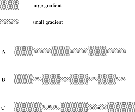
  Figure 1: Both shortening the light, small mass gradient part (example B), and lengthening the heavy, high gradient part of the lattice (example C) lead to an effective increase of average mass gradient as compared to A, and therefore to a higher remoteness of the configuration, which reflects in an increased critical temperature.

  We can give a rough estimate of the effect, by considering that the light part has masses which are around one-half of those of the heavy part, and the change in the structure, as compared to the longer lattice form (the one of (Tl₄Ba)Ba₄Ca₂Cu₁₁O_ν), amounts to suppressing some 2-3 layers in this light part, out of a total of $\sim$ 20 lattice planes. This is a change of around 1/2 of $10\%$, i.e. $\sim 5\%$, corresponding to a jump in the temperature of some 12 ^oK. This leads from the former 242 ^oK to around 254 ^oK.

  This example shows that, although working within a single unit of lattice length, as implied in 3.25–3.27, is in most cases correct, in principle the comparison of geometries is something more subtle. In the case of (Tl₄Ba)Ba₂Ca₂Cu₇O₁₃₊, just considering one unit of lattice length is not enough.

3.3.3 The (SnPbIn)BaTmCuO family: from 163 ^oK to 195 ^oK.

The lattice structure of (Sn_1.0Pb_0.5In_0.5)Ba₄Tm₄Cu₆O₁₈₊, $T_{c}$ = 163 ^oK consists of a stack of (0,5(Sn_1.0Pb_0.5In_0.5)-O) (Ba) (CuO_x) (Tm) (CuO_x) (Ba) (0,5(Sn_1.0Pb_0.5In_0.5)-O) (Ba) (CuO_x) (Tm) (CuO_y) (Tm) (CuO_y) (Tm) (CuO_x) (Ba).
The lattice structure of (Sn_1.0Pb_0.5In_0.5)Ba₄Tm₅Cu₇O₂₀₊, $T_{c}$ = 185 ^oK consists of a stack of (0,5(Sn_1.0Pb_0.5In_0.5)-O) (Ba) (CuO_x) (Tm) (CuO_x) (Ba) (0,5(Sn_1.0Pb_0.5In_0.5)-O) (Ba) (CuO_x) (Tm) (CuO_y) (Tm) (CuO_y) (Tm) (CuO_y) (Tm) (CuO_x) (Ba). The lattice structure of (Sn_1.0Pb_0.5In_0.5)Ba₄Tm₆Cu₈O₂₂₊, $T_{c}$ = 195 ^oK, consists of a stack of (0,5(Sn_1.0Pb_0.5In_0.5)-O) (Ba) (CuO_x) (Tm) (CuO_x) (Ba) (0,5(Sn_1.0Pb_0.5In_0.5)-O) (Ba) (CuO_x) (Tm) (CuO_y) (Tm) (CuO_y) (Tm) (CuO_y) (Tm) (CuO_y) (Tm) (CuO_x) (Ba). It is difficult to compare with the elements of the previous series. On the other hand, since the differences among the elements of this series consist in adding a [(CuO_y) (Tm)] pair of layers within the same lattice subset, it is relatively easy to compare the elements within this group. In practice we are adding a Tm line at each step, increasing the lattice complexity by one layer out of a total of 10 in the first case, and of 10+1 in the second case. We expect therefore an increase of $T_{c}$ by a factor 11/10 and 12/11 respectively. This corresponds to a jump from $\sim$163 to $\sim$180 ^oK, and to $\sim$195 ^oK in the second case.

4 Comments

The analysis of the previous section provides support to the hypothesis that quantum gravity effects may be at the ground of the understanding of the relation between lattice complexity and critical temperature of superconductors. Roughly speaking, working in a quantum gravity framework effectively means having a Planck constant dependent on the distribution of energy along space. If we introduce an energy density $\rho(E)$, this in practice means that we are effectively promoting $\hbar$ to

$$\hbar~{}\to~{}\hbar(\rho(E))\,.$$ (4.53)

Alternatively, since energy distribution along space and space geometry are equivalent, we can also say that we work with a geometry-dependent Planck constant:

$$\hbar~{}\to~{}\hbar(g_{\mu\nu})\,,$$ (4.54)

or, to work with quantities independent on the choice of coordinate system, with a curvature-dependent Planck constant. Although all the expressions considered in this paper are worked out within a non-field theoretical framework, from an heuristic point of view this dependence can be understood as follows. Quantization of gravity introduces an effective dependence on $\hbar$ in the modes of propagation of the metric tensor $g_{\mu\nu}$. This means that, even if we start with a space with a classical background metric, after quantization, and as a consequence of the back reaction due to the interaction with matter and radiation, we will end up with a space with $\hbar$-dependent geometry, $g_{\mu\nu}(\hbar)$. Taking the point of view of considering geometry as a primary, independent input corresponds to inverting the relation $g_{\mu\nu}=g_{\mu\nu}(\hbar)$ to $\hbar=\hbar(g_{\mu\nu})$. The functional dependence is not simple; on the other hand, its explicit expression is not even fundamental, because it expresses only an effective parametrization: in general, in order to derive, case by case, the appropriate effective parametrization, one has to refer to 1.1 . The ground value of the Planck constant is the one corresponding to the “vacuum”, which in our case is the universe with uniform curvature, corresponding to the cosmological constant . A uniform curvature gives a universal contribution that can be subtracted, i.e. re-absorbed into a redefinition of the Planck constant. This is what is done when gravity is decoupled from the quantum theory, and one recovers the traditional quantum theory.

A dependence of the Planck constant on the geometry means that also the amount of quantum delocalization of wave functions, the mechanism at the ground of superconductivity, depends on the geometry. However, the relation between critical temperature and lattice complexity of superconductors cannot be observed in a clean, direct way: superconductivity is a regime in most cases “unstable” in pure materials, and the way it is detected makes measurements very sensitive to several additional conditions. The simple relation we suggest between critical temperature and “geometry” only works at the net of any other effect, such as degree of doping/pinning of magnetic flux, etc. A quantitative prediction is only possible when the contribution of these effects can been subtracted. The agreement between expectations and theoretical predictions we find has therefore to be read “in the average”, and works better in comparing temperatures between materials belonging to the same “family”, for which therefore other conditions can be assumed to be similar (the case of the Hg-12010/1212/1223 series is exemplar of this situation). Nevertheless, the agreement between predictions and experimental observations is impressive. Our analysis provides a further indication that, differently from what one is used to expect, quantum gravity is not just a matter of Planck scale phenomena, but in principle comes into play, to contribute for non-negligible corrections, in any quantum system corresponding to a non-trivial geometry of space-time.

In the universe described in Ref. [1], geometry evolves with time. Not only the cosmological constant and the matter density of the universe, and therefore the ground curvature, evolve with time, but also all elementary masses depend on the age of the universe. It is not hard to realize that, since also couplings, in particular the fine structure constant, evolve with the age of the universe, also the masses of atoms and molecules do evolve. In particular, electron, proton and neutron mass evolve as appropriate inverse powers of the age of the universe:

$$m_{i}\sim{\cal T}^{-a_{i}}\,,$$

where $a_{i}<1$ and $i$ indicates the electron, or the proton, or the neutron. Similarly it goes for the electric coupling:

$$\alpha\sim{\cal T}^{-a_{\alpha}}\,.$$

As a consequence, also the masses of atoms and molecules are expected to scale with time, perhaps with a more complicated dependence than that of elementary particles, but anyway in such a way to decrease with time, with an increasing relative rate. This means that the mass ratio of heavier to lighter atoms is expected to increase with time. Therefore, owing to the change of geometry, or, equivalently, of the effective Planck constant, we should expect also an increase in the ratio of different degrees of delocalization of wavefunctions. How fast should this go can be estimated by considering that, approximately, mass ratios scale as powers of the age of the universe. With a similar degree of approximation, we can assume that also lattice gradient ratios scale as powers of the age of the universe. A factor 2 in the ratio of the mean weights of configurations at present time:

$${\xi_{i}\over\xi_{j}}~{}\approx~{}{\langle\nabla m_{i}\rangle\over\langle\nabla m_{j}\rangle}~{}\sim~{}2\,,$$

corresponds to a very small exponent $a_{(\xi_{i}/\xi_{j})}$ of the evolution:

$${\xi_{i}\over\xi_{j}}~{}\approx~{}{\cal T}^{a_{(\xi_{i}/\xi_{j})}}\,.$$

This is given in fact as $\log 2=a_{(\xi_{i}/\xi_{j})}\log{\cal T}$, where the age of the universe ${\cal T}$ is expressed in units of appropriately converted Planck length. At present time ${\cal T}\sim 10^{61}$. This kind of evolution is therefore only detectable on a large, cosmological, time scale, and negligible for usual purposes.

Transition
Temperature	Material	Class
in Kelvin
254	(Tl4 Ba) Ba2 Ca2 Cu7 O13+
242	(Tl4 Ba) Ba4 Ca2 Cu11 Oν
233	Tl5 Ba4 Ca2 Cu11 Oν
218	(Sn5 In) Ba4 Ca2 Cu11 Oν
212	(Sn5 In) Ba4 Ca2 Cu10 Oν
200	Sn6 Ba4 Ca2 Cu10 Oν
160	Sn3 Ba4 Ca2 Cu7 Oν
195	(Sn1.0 Pb0.5 In0.5)Ba4Tm6Cu8O22+
185	(Sn1.0 Pb0.5 In0.5)Ba4Tm5Cu7O20+	Copper-oxide superconductors
163	(Sn1.0 Pb0.5 In0.5)Ba4Tm4Cu6O18+
125	Tl2Ba2Ca2Cu3O10
108	Tl2Ba2CaCu2O8
80	Tl2Ba2CuO6
110	Bi2 Sr2 Ca2 Cu3 O10(Bi2223)
92	Bi2Sr2CaCu2O2 (Bi2212)
92	YBa2 Cu3 O7 (YBCO)
57	SmFeAs(O,F)=SmOFeAs	Iron-based superconductors
44	LaFeAs(O,F)=LaOFeAs
18	Nb3 Sn
10	NbTi	Metallic low-temp. superconductors
4.2	Hg

References

- [1] A. Gregori, About combinatorics, and observables, arXiv:0712.0471 [hep-th].
- [2] J. Bardeen, L. N. Cooper, and J. R. Schrieffer, Theory of Superconductivity, Phys. Rev. 108 (1957) 1175.
- [3] A. Gregori, Relativity as classical limit in a combinatorial scenario, arXiv:0911.0518v1 [physics.gen-ph].
- [4] A. Gregori, An entropy-weighted sum over non-perturbative vacua, arXiv:0705.1130 [hep-th].
- [5] M. Tinkham, Introduction to Superconductivity. Dover Publications, 2004.
- [6] H. Takahashi, K. Igawa, K. Arii, Y. Kamihara, M. Hirano, and H. Hosono, Superconductivity at 43 K in an iron-based layered compound LaO1-xFxFeAs, Nature 453 (2008) 376–378.
- [7] R. Zhi-An et al., Superconductivity at 43 K in an iron-based layered compound LaO1-xFxFeAs, Chinese Phys. Lett. 25 (2008) 2215–2216.
- [8] R. Zhi-An et al., Fluorinated superconductors , NPG Asia Materials (Published online 14 July 2008).
- [9] M. K. Wu, J. R. Ashburn, C. J. Torng, P. H. Hor, R. L. Meng, L. Gao, Z. J. Huang, Y. Q. Wang, and C. W. Chu, Superconductivity at 93 K in a new mixed-phase Y-Ba-Cu-O compound system at ambient pressure, Phys. Rev. Lett. 58 (Mar, 1987) 908–910.
- [10] H. Maeda, Y. Tanaka, M. Fukutomi, and T. Asano, A New High- Oxide Superconductor without a Rare Earth Element, Japanese Journal of Applied Physics 27 (1988), no. Part 2, No. 2, L209–L210.
- [11] Z. Sheng, A. Hermann, A. El Ali, C. Almasan, J. Estrada, T. Datta, and R. Matson, Superconductivity at 90 K in the Tl-Ba-Cu-O system, Physical Review Letters 60 (1988) 937.
- [12] S. S. P. Parkin, V. Y. Lee, A. I. Nazzal, R. Savoy, R. Beyers, and S. J. La Placa, A new class of crystal structures exhibiting volume superconductivity at up to 110 K, Phys. rev. Lett. 61 (1988) 750–753.
- [13] N. Khare, ed., Handbook of High-Temperature Superconductor Electronics. Marcel Dekker, 2003.
- [14] Z. Sheng and A. M. Hermann, Superconductivity in the rare-earth-free Tl-Ba-Cu-O system above liquid-nitrogen temperature, Nature 332 (1988) 55.
- [15] S. N. Putilin, E. V. Antipov, O. Chmaissem, and M. Marezio, Superconductivity at 94 K in HgBa2Cu04+, Nature 362 (1993) 226.
- [16] J. L. Wagner, T. M. Clemens, D. C. Mathew, O. Chmaissem, B. Dabrowski, J. Jorgensen, and D. Hinks, Universal Phase Diagrams and Ideal High Temperature Superconductors: HgBa2CuO4+, in Phase Transitions and Self-Organization in Electronic and Molecular Networks, M. F. Thorpe and J. C. Phillips, eds., pp. 331–339. Springer US, 2002.
- [17] C. W. Chu, L. Gao, F. Chen, Z. J. Huang, R. L. Meng, and Y. Y. Xue, Superconductivity above 150 K in HgBa2Ca2Cu3O8+ at high pressures, Nature 365 (1993) 323.